Interaction and Entanglement in the
Multiparticle Spacetime Algebra

Timothy F. Havel1 and Chris J. L. Doran2

1MIT (NW14-2218), 150 Albany St., Cambridge, MA 02139, USA. tfhavel@mit.edu

2Astrophysics Group, Cavendish Laboratory, Madingley Road, Cambridge CB3 0HE, UK. c.doran@mrao.cam.ac.uk

Abstract

The multiparticle spacetime algebra (MSTA) is an extension of Dirac theory to a multiparticle setting, which was first studied by Doran, Gull and Lasenby. The geometric interpretation of this algebra, which it inherits from its one-particle factors, possesses a number of physically compelling features, including simple derivations of the Pauli exclusion principle and other nonlocal effects in quantum physics. Of particular importance here is the fact that all the operations needed in the quantum (statistical) mechanics of spin $1/2$ particles can be carried out in the “even subalgebra” of the MSTA. This enables us to “lift” existing results in quantum information theory regarding entanglement, decoherence and the quantum / classical transition to space-time. The full power of the MSTA and its geometric interpretation can then be used to obtain new insights into these foundational issues in quantum theory. A system of spin $1/2$ particles located at fixed positions in space, and interacting with an external magnetic field and/or with one another via their intrinsic magnetic dipoles provides a simple paradigm for the study of these issues. This paradigm can further be easily realized and studied in the laboratory by nuclear magnetic resonance spectroscopy.

1 The Physics of Quantum Information

Information, to be useful, must be encoded in the state of a physical system. Thus, although information can have more than one meaning, it always has something to say about the state of the system it is encoded in. Conversely, the average information needed to specify the state of a system drawn at random from some known probability distribution is proportional to the entropy of the corresponding statistical mechanical “system”. It follows that entropy can be understood as a measure of the system’s information storage capacity. The physics of information is a fertile area of research which promises to become increasingly important as computers and nanotechnology approach the limits of what is physically possible [4, 8].

In practice, information is usually binary encoded into an array of two-state systems, each of which can hold one bit of data, where the two “states” correspond to the minimum or maximum value of a continuous degree of freedom. Ordinarily such physical bits obey classical mechanics, but many examples of two-state quantum systems are known, for example adjacent pairs of energy levels in atoms, photon polarizations, or the magnetic dipole orientations of fermions. These quantum bits, or qubits as they are called, have a number of distinctive and nonintuitive properties [3, 14, 23]. In particular, the number of parameters needed to specify (the statistics of measurement outcomes on) the joint state of an array of $n$ qubits is generally $2^{n}$ — exponentially larger than the $n$ needed for an array of classical bits! These new degrees of freedom are due to the existence of non-separable or entangled states, which may be thought of as providing direct paths between pairs of states related by flipping more than one bit at a time. A further mysterious property of these quantum states stems from the fact that it is impossible (so far as is known!) to determine just where on the pathways between states the qubits are. This is because the act of measuring the qubits’ states (however this may be done) always “collapses” them into one of their extremal states [17].

A quantum computer is an array of distinguishable qubits that can be put into a known state, evolved under a sequence of precisely controlled interactions, and then measured. It has been shown that such a computer, if one could be built, would be able to solve certain problems asymptotically more rapidly than any classical device. Unfortunately, quantum systems are exceedingly difficult to isolate, control and monitor, so that at this time only simple prototype quantum computers have been operated in the laboratory. Although far from competitive with today’s laptops, these prototypes are of great scientific interest. This is because quantum computers provide a paradigm for the study of a number of poorly understood issues in quantum mechanics, including why the particular classical world we inhabit is singled out from the myriads allowed by quantum mechanics. This is widely believed to be the result of decoherence: the decay of accessible information due to the entanglement generated by the interactions between the system with its environment [9, 15, 16]. The reason such issues are poorly understood, even though the microscopic laws of quantum mechanics are complete and exact, lies in our very limited ability to integrate these laws into precise solutions for large and complex quantum systems, or even to gain significant insights into their long-term statistical behavior. The intrinsic complexity of quantum dynamics is in fact precisely what makes quantum computers so powerful to begin with!

This paper will explore the utility of the multiparticle spacetime algebra (MSTA) description of qubit states, as introduced by Doran, Gull and Lasenby [6, 7, 20], for the purposes of understanding entanglement, decoherence and quantum complexity more generally. As always with applications of geometric algebra, our goal will be to discover simple geometric interpretations for otherwise incomprehensible algebraic facts. To keep our study concrete and our observations immediately amenable to experimental verification, we shall limit ourselves to the qubit interactions most often encountered in physical implementations, namely the interaction between the magnetic dipoles of spin $1/2$ particles such as electrons, neutrons and certain atomic nuclei. These will be assumed to have fixed positions, so their spatial degrees of freedom can be ignored. Examples of such systems, often involving $10^{20}$ or more spins (qubits), are widely encountered in chemistry and condensed matter physics, and can readily be studied by various spectroscopies, most notably nuclear magnetic resonance (NMR) [1, 10, 18, 22].

2 The Multiparticle Space-Time Algebra

It will be assumed in the following that the reader has at least a basic familiarity with geometric algebra, as found in e.g. [2, 6, 13]. This brief account of the MSTA is intended mainly to introduce the notation of the paper, while at the same time providing a taste of how the MSTA applies to quantum information processing. More introductory accounts may be found in [7, 10, 11, 21].

The $n$-particle MSTA is the geometric algebra ${\mathcal{G}}(n,3n)$ generated by $n$ copies of Minkowski space-time ${\mathcal{R}}^{1,3}$. We let $\{\gamma_{\mu}^{a}\,|\,\mu=0,\ldots,3\}$ denote a basis set of vector generators for this algebra, satisfying

$$\gamma_{\mu}^{a}\!\cdot\!\gamma_{\nu}^{b}~{}=~{}\eta_{\mu\nu\,}\delta^{ab}\,.$$ (1)

The superscripts refer to separate particle spaces ($a,b=1,\ldots,n$) and the subscripts label spacetime vectors ($\mu,\nu=0,\ldots,3$), while $\eta_{\mu\nu}$ is the standard Minkowski metric of signature $(+--\,-)$. The $\{\gamma_{\mu}^{a}\}$ can be thought of as a basis for relativistic configuration space, and the MSTA is the geometric algebra of this space.

The even subalgebra of each copy of the spacetime algebra is isomorphic to the algebra of Euclidean three-dimensional space ${\mathcal{G}}(3)$ [12]. The specific map depends on a choice of timelike vector, and the algebra then describes the rest space defined by that vector. It is convenient in most applications to identify this vector with $\gamma_{0}$, and we define

$$\boldsymbol{\sigma}_{\!k}^{a}~{}=~{}\gamma_{k}^{a}\gamma_{0}^{a}\,.$$ (2)

Each set of spatial vectors $\boldsymbol{\sigma}_{\!1}^{a},\boldsymbol{\sigma}_{\!2}^{a},\boldsymbol{\sigma}_{\!3}^{a}$ generates a three-dimensional geometric algebra. It is easily seen that the generators of different particle spaces commute, so that the algebra they generate is isomorphic to the Kronecker product ${\mathcal{G}}(3)\,\otimes\cdots\otimes\,{\mathcal{G}}(3)$. For this paper we will work almost entirely within this (non-relativistic) space, but it should be borne in mind throughout that all results naturally sit in a fully relativistic framework.

To complete our definitions, we denote the pseudoscalar for each particle by

$${\boldsymbol{\iota}}^{a}~{}=~{}\gamma_{0}^{a}\gamma_{1}^{a}\gamma_{2}^{a}\gamma_{3}^{a}~{}=~{}\boldsymbol{\sigma}_{\!1}^{a}\boldsymbol{\sigma}_{\!2}^{a}\boldsymbol{\sigma}_{\!3}^{a}\,.$$ (3)

For the bivectors in each spatial algebra we make the abbreviation ${\boldsymbol{\iota}}^{a}\boldsymbol{\sigma}_{\!k}^{a}=\boldsymbol{\iota}\!\boldsymbol{\sigma}_{\!k}^{a}$. The reverse operation in the MSTA is denoted with a tilde. This flips the sign of both vectors and bivectors in ${\mathcal{G}}(3)$, and so does not correspond to spatial reversion.

There are many ways to represent multiparticle states within the MSTA. Here we are interested in an approach which directly generalizes that of Hestenes for single-particle non-relativistic states. We will represent states using multivectors constructed from products of the even subalgebras of each ${\mathcal{G}}(3)$. That is, states are constructed from sums and products of the set $\{1,\boldsymbol{\iota}\!\boldsymbol{\sigma}_{\!k}^{a}\}$, where $k=1\ldots 3$ and $a$ runs over all particle spaces. This algebra has real dimension $4^{n}$, which is reduced to the expected $2^{n+1}$ by enforcing a consistent representation for the unit imaginary. This is ensured by right-multiplying all states with the correlator idempotent

$${\boldsymbol{E}}~{}\equiv~{}\mathchoice{\textstyle\frac{1}{2}}{\frac{1}{2}}{\frac{1}{2}}{\frac{1}{2}}(1-\boldsymbol{\iota}\!\boldsymbol{\sigma}_{\!3}^{1}\boldsymbol{\iota}\!\boldsymbol{\sigma}_{\!3}^{2})\,\mathchoice{\textstyle\frac{1}{2}}{\frac{1}{2}}{\frac{1}{2}}{\frac{1}{2}}(1-\boldsymbol{\iota}\!\boldsymbol{\sigma}_{\!3}^{1}\boldsymbol{\iota}\!\boldsymbol{\sigma}_{\!3}^{3})~{}\cdots~{}\mathchoice{\textstyle\frac{1}{2}}{\frac{1}{2}}{\frac{1}{2}}{\frac{1}{2}}(1-\boldsymbol{\iota}\!\boldsymbol{\sigma}_{\!3}^{1}\boldsymbol{\iota}\!\boldsymbol{\sigma}_{\!3}^{n})~{}.$$ (4)

The correlator is said to be idempotent because it satisfies the projection relation

$${\boldsymbol{E}}^{2}~{}=~{}{\boldsymbol{E}}.$$ (5)

In the case of two spins, for example, we have ${\boldsymbol{E}}=-\boldsymbol{\iota}\!\boldsymbol{\sigma}_{\!3}^{1}\boldsymbol{\iota}\!\boldsymbol{\sigma}_{\!3}^{2}{\boldsymbol{E}}$, so that any term right-multiplied by $-\boldsymbol{\iota}\!\boldsymbol{\sigma}_{\!3}^{1}\boldsymbol{\iota}\!\boldsymbol{\sigma}_{\!3}^{2}$ is projected by ${\boldsymbol{E}}$ back to the same element. The correspondence with the usual complex vector space representation is obtained by observing that (for e.g. two spins) every spinor may be written uniquely as

$$\boldsymbol{\psi}~{}=~{}\left(\boldsymbol{\psi}_{1}-\boldsymbol{\iota}\!\boldsymbol{\sigma}_{\!2}^{2}\boldsymbol{\psi}_{2}-\boldsymbol{\iota}\!\boldsymbol{\sigma}_{\!2}^{1}\boldsymbol{\psi}_{3}+\boldsymbol{\iota}\!\boldsymbol{\sigma}_{\!2}^{1}\boldsymbol{\iota}\!\boldsymbol{\sigma}_{\!2}^{2}\boldsymbol{\psi}_{4}\right){\boldsymbol{E}}~{},$$ (6)

where the $\boldsymbol{\psi}_{k}$ are “complex numbers” of the form $\alpha_{k}+\beta_{k}{\boldsymbol{J}}$ with $\alpha_{k}$, $\beta_{k}$ real, and the role of the imaginary is played by the (non-simple) bivector

$${\boldsymbol{J}}~{}\equiv~{}\boldsymbol{\iota}\!\boldsymbol{\sigma}_{\!3}^{1}{\boldsymbol{E}}~{}=~{}\boldsymbol{\iota}\!\boldsymbol{\sigma}_{\!3}^{2}{\boldsymbol{E}}~{}=~{}\mathchoice{\textstyle\frac{1}{2}}{\frac{1}{2}}{\frac{1}{2}}{\frac{1}{2}}(\boldsymbol{\iota}\!\boldsymbol{\sigma}_{\!3}^{1}+\boldsymbol{\iota}\!\boldsymbol{\sigma}_{\!3}^{2}).$$ (7)

The complex generator ${\boldsymbol{J}}$ satisfies ${\boldsymbol{J}}^{2}~{}=~{}-{\boldsymbol{E}}$, which ensures consistency with the standard formulation of quantum theory. As in the single-particle case, the complex structure is always represented by right-multiplication by ${\boldsymbol{J}}$. While this approach may look strange at first, it does provide a number of new geometric insights into the nature of multiparticle Hilbert space [7].

3 Two Interacting Qubits

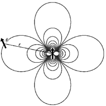
As an application of the MSTA approach, we consider a simple model system of interacting qubits. This exhibits all of the complexity of multiparticle quantum systems generally, including the role of entanglement and the distinction between classical and quantum theories. Associated with the intrinsic angular momentum of any spin $1/2$ particle is a magnetic dipole $\boldsymbol{\mu}$. In the far-field limit, the energy for the interaction between two such dipoles is given classically by the expression

$$E_{D}~{}=~{}\frac{\mu_{0}}{4\pi}\left(\frac{\boldsymbol{\mu}_{1}\!\cdot\!\boldsymbol{\mu}_{2}}{r^{3}}~{}-~{}3\,\frac{\boldsymbol{\mu}_{1}\!\cdot\!{\boldsymbol{r}}\,\boldsymbol{\mu}_{2}\!\cdot\!{\boldsymbol{r}}}{r^{5}}\right)~{},$$ (8)

where $\mu_{0}$ is the permeability of the vacuum, ${\boldsymbol{r}}$ is the radial vector between the dipoles, and $r=|{\boldsymbol{r}}|$ (see Fig. 1). To obtain the quantum theory of this system (via “first quantization”) we replace the magnetic moment $\boldsymbol{\mu}$ by its operator equivalent, given by the component relation

$$\hat{\mu}_{k}~{}=~{}\gamma\hat{s}_{k}.$$ (9)

Here $\gamma$ is the gyromagnetic ratio and $\hat{s}_{k}$ is the spin operator in the $k$-th direction. For a spin $1/2$ particle the spin operators are simply

$$\hat{s}_{k}~{}=~{}\mathchoice{\textstyle\frac{1}{2}}{\frac{1}{2}}{\frac{1}{2}}{\frac{1}{2}}\hbar\hat{\sigma}_{k},$$ (10)

where the $\hat{\sigma}_{k}$ are the Pauli matrix operators. The classical energy of (8) gives rise to a quantum Hamiltonian containing 2 terms. The first involves $\boldsymbol{\mu}_{1}\!\cdot\!\boldsymbol{\mu}_{2\,}$, which is replaced by the operator

$$\sum_{k=1}^{3}\hat{\mu}_{k}^{1}\,\hat{\mu}_{k}^{2}~{}=~{}\frac{\hbar^{2}\gamma_{1}\gamma_{2}}{4}\sum_{k=1}^{3}\,\hat{\sigma}_{k}\otimes\hat{\sigma}_{k},$$ (11)

where $\gamma_{1}$ and $\gamma_{2}$ are the gyromagnetic ratios of particles 1 and 2 respectively. This operator acts on a four-dimensional complex vector space. To form the MSTA equivalent of this we write

$$\sum_{k=1}^{3}\,\hat{\sigma}_{k}\otimes\hat{\sigma}_{k}~{}=~{}-\sum_{k=1}^{3}\,i\hat{\sigma}_{k}\otimes i\hat{\sigma}_{k}~{},$$ (12)

where $i$ is an (uninterpreted) imaginary unit. Each factor of $i\hat{\sigma}_{k}$ has an equivalent action in the MSTA given by left-multiplication with $\boldsymbol{\iota}\!\boldsymbol{\sigma}_{\!k}$ in the corresponding particle’s space. It follows that we can replace

$$\sum_{k=1}^{3}\,\hat{\sigma}_{k}\otimes\hat{\sigma}_{k}|\,\psi\,\rangle~{}\mapsto~{}-\sum_{k=1}^{3}\boldsymbol{\iota}\!\boldsymbol{\sigma}_{\!k}^{1}\,\boldsymbol{\iota}\!\boldsymbol{\sigma}_{\!k}^{2}\,\boldsymbol{\psi}~{}.$$ (13)

We can already see, therefore, that the Hamiltonian is going to become a 4-vector in the MSTA.

Refer to caption
Refer to caption
Figure 1: One dipole in the field of another, the radial vector ${\boldsymbol{r}}$ between them, and the angle $\theta$ it makes with the dipole (left); corresponding potential energy surface (assuming the dipoles are confined to the plane as depicted on the left) showing that there are two minima, two maxima, and four saddle points (right).

For the second term we let ${\boldsymbol{n}}={\boldsymbol{r}}/r$, so that ${\boldsymbol{n}}$ is the unit vector parallel to the line between the dipoles’ centers. We next form the operator for $\boldsymbol{\mu}_{1}\!\cdot{\boldsymbol{n}}\,\boldsymbol{\mu}_{2}\!\cdot{\boldsymbol{n}}$, which is

$$\sum_{k,\ell=1}^{3}n_{k}n_{\ell}\,\hat{\mu}_{k}^{1}\,\hat{\mu}_{\ell}^{2}~{}=~{}\frac{\hbar^{2}\gamma_{1}\gamma_{2}}{4}\sum_{k,\ell=1}^{3}n_{k}\,n_{\ell}\,\hat{\sigma}_{k}\otimes\hat{\sigma}_{\ell}\,.$$ (14)

The MSTA equivalent of this is simply

$$-\frac{\hbar^{2}\gamma_{1}\gamma_{2}}{4}\sum_{k,\ell=1}^{3}n_{k}\,n_{\ell}\,\boldsymbol{\iota}\!\boldsymbol{\sigma}_{\!k}^{1}\,\boldsymbol{\iota}\!\boldsymbol{\sigma}_{\!\ell}^{2}~{}=~{}-\frac{\hbar^{2}\gamma_{1}\gamma_{2}}{4}\,\boldsymbol{\iota}\!{{\boldsymbol{n}}}^{1}\,\boldsymbol{\iota}\!{{\boldsymbol{n}}}^{2}\,.$$ (15)

The role of the Hamiltonian in the MSTA is therefore assumed by the 4-vector

$${\boldsymbol{H}}_{\mathsf{D}}~{}\equiv~{}-\frac{d}{4}\,\Bigl{(}\sum_{k=1}^{3}\,\boldsymbol{\iota}\!\boldsymbol{\sigma}_{\!k}^{1}\boldsymbol{\iota}\!\boldsymbol{\sigma}_{\!k}^{2}\,-\,3\,\boldsymbol{\iota}\!{{\boldsymbol{n}}}^{1}\boldsymbol{\iota}\!{{\boldsymbol{n}}}^{2}\Bigr{)}\,,$$ (16)

where $d\equiv\mu_{0}\hbar\gamma_{1}\gamma_{2}/4\pi r^{3}$ $sec^{-1}$. This definition of ${\boldsymbol{H}}_{\mathsf{D}}$ is chosen so that Schrödinger’s equation takes the simple form

$$-\partial_{t}\,\boldsymbol{\psi}~{}=~{}{\boldsymbol{H}}_{\mathsf{D}}\,\boldsymbol{\psi}\,{\boldsymbol{J}}\,.$$ (17)

¿From this one can immediately see a key feature of the MSTA approach, which is that all references to the tensor product have been removed. All one ever needs is the geometric product, which inherits all of the required properties from the relativistic definition of the MSTA.

3.1 The Propagator

In the more conventional, matrix-based approach to quantum theory the propagator in the current setup would be simply $\exp(-i\hat{H}t/\hbar)$. In finding the MSTA equivalent of this we appear to have a serious problem. In equation (17) the 4-vector ${\boldsymbol{H}}_{\mathsf{D}}$ acts from the left on $\boldsymbol{\psi}$, whereas $\boldsymbol{J}$ sits on the right. In fact, this is more of a notational issue than a foundational one. We simply define an operator $\boldsymbol{j}$ to denote right-multiplication by $\boldsymbol{J}$ when acting on a multiparticle state, namely

$$\boldsymbol{j}\boldsymbol{\psi}~{}\equiv~{}\boldsymbol{\psi}\boldsymbol{J}\,.$$ (18)

We are then free to write $\boldsymbol{j}$ anywhere we chose within a multiplicative term, and to let it distribute over addition like a multiplicative operator. This notational device is extremely useful in practice, though occasionally one has to be careful in applying it.

The propagator can be obtained in a number of ways. One is to write

$${\boldsymbol{H}}_{\mathsf{D}}~{}=~{}\frac{d}{2}\,\boldsymbol{\Pi}\,-\,\frac{d}{4}\,+\,\frac{3d}{4}\,\boldsymbol{\iota}\!{{\boldsymbol{n}}}^{1}\boldsymbol{\iota}\!{{\boldsymbol{n}}}^{2}\,,$$ (19)

where

$$\boldsymbol{\Pi}~{}=~{}\mathchoice{\textstyle\frac{1}{2}}{\frac{1}{2}}{\frac{1}{2}}{\frac{1}{2}}\bigl{(}1-\boldsymbol{\iota}\!\boldsymbol{\sigma}_{\!1}^{1}\boldsymbol{\iota}\!\boldsymbol{\sigma}_{\!1}^{2}-\boldsymbol{\iota}\!\boldsymbol{\sigma}_{\!2}^{1}\boldsymbol{\iota}\!\boldsymbol{\sigma}_{\!2}^{2}-\boldsymbol{\iota}\!\boldsymbol{\sigma}_{\!3}^{1}\boldsymbol{\iota}\!\boldsymbol{\sigma}_{\!3}^{2}\bigr{)}\,.$$ (20)

The multivector $\boldsymbol{\Pi}$ constitutes a geometric representation of the particle interchange operator, since $\boldsymbol{\Pi}\,\boldsymbol{\zeta}^{1}\boldsymbol{\upsilon}^{2}=\boldsymbol{\upsilon}^{1}\boldsymbol{\zeta}^{2}\boldsymbol{\Pi}$, and hence satisfies $\boldsymbol{\Pi}^{2}=1$. It follows that $\boldsymbol{\Pi}$ commutes with $\boldsymbol{\iota}\!{{\boldsymbol{n}}}^{1}\boldsymbol{\iota}\!{{\boldsymbol{n}}}^{2}$, and the propagator can be written as

$$\boldsymbol{\exp}(-\boldsymbol{j}\,{\boldsymbol{H}}_{\mathsf{D\,}}t)~{}=~{}\boldsymbol{\exp}(-\boldsymbol{j}\,dt/4)\,\boldsymbol{\exp}(\boldsymbol{j}\,\boldsymbol{\Pi}\,dt/2)\,\boldsymbol{\exp}(\boldsymbol{j}\,\boldsymbol{\iota}\!{{\boldsymbol{n}}}^{1}\boldsymbol{\iota}\!{{\boldsymbol{n}}}^{2\,}3dt/4).$$ (21)

All three exponentials in this expression commute.

Alternatively, one can look for eigenstates of the Hamiltonian. At this point it is convenient to choose a coordinate system in which ${{\boldsymbol{r}}}$ is parallel to the ${\mathsf{z}}$-axis, so that

$${\boldsymbol{n}}~{}=~{}\boldsymbol{\sigma}_{\!3}\,,\quad{\boldsymbol{H}}_{\mathsf{D}}~{}=~{}\frac{d}{4}\,\bigl{(}2\,\boldsymbol{\iota}\!\boldsymbol{\sigma}_{\!3}^{1}\boldsymbol{\iota}\!\boldsymbol{\sigma}_{\!3}^{2}\,-\,\boldsymbol{\iota}\!\boldsymbol{\sigma}_{\!1}^{1}\boldsymbol{\iota}\!\boldsymbol{\sigma}_{\!1}^{2}\,-\,\boldsymbol{\iota}\!\boldsymbol{\sigma}_{\!2}^{1}\boldsymbol{\iota}\!\boldsymbol{\sigma}_{\!2}^{2}\bigr{)}~{}.$$ (22)

One can “diagonalize” the Hamiltonian operator in this coordinate frame by defining

$\displaystyle{\boldsymbol{H}}_{\mathsf{D}}^{\prime}~{}=~{}$ $\displaystyle~{}{\boldsymbol{e}}^{(\pi/4)\,\boldsymbol{j}\boldsymbol{\iota}\!\boldsymbol{\sigma}_{\!1}^{1}\boldsymbol{\iota}\!\boldsymbol{\sigma}_{\!2}^{2}\,}{\boldsymbol{H}}_{\mathsf{D}}\,{\boldsymbol{e}}^{-(\pi/4)\,\boldsymbol{j}\boldsymbol{\iota}\!\boldsymbol{\sigma}_{\!1}^{1}\boldsymbol{\iota}\!\boldsymbol{\sigma}_{\!2}^{2}}$
$\displaystyle~{}=~{}$ $\displaystyle~{}\frac{d}{4}\,\Big{(}2\,\boldsymbol{\iota}\!\boldsymbol{\sigma}_{\!3}^{1}\boldsymbol{\iota}\!\boldsymbol{\sigma}_{\!3}^{2}\,-\,\boldsymbol{j}\boldsymbol{\iota}\!\boldsymbol{\sigma}_{\!1}^{1}\boldsymbol{\iota}\!\boldsymbol{\sigma}_{\!2}^{2}\,\big{(}\boldsymbol{\iota}\!\boldsymbol{\sigma}_{\!1}^{1}\boldsymbol{\iota}\!\boldsymbol{\sigma}_{\!1}^{2}+\boldsymbol{\iota}\!\boldsymbol{\sigma}_{\!2}^{1}\boldsymbol{\iota}\!\boldsymbol{\sigma}_{\!2}^{2}\big{)}\Big{)}$
$\displaystyle~{}=~{}$ $\displaystyle~{}\frac{d}{4}\,\Big{(}2\,\boldsymbol{\iota}\!\boldsymbol{\sigma}_{\!3}^{1}\boldsymbol{\iota}\!\boldsymbol{\sigma}_{\!3}^{2}\,+\,\boldsymbol{j}\big{(}\boldsymbol{\iota}\!\boldsymbol{\sigma}_{\!3}^{1}-\boldsymbol{\iota}\!\boldsymbol{\sigma}_{\!3}^{2}\big{)}\Big{)}~{}.$ (23)

The eigenvalues and eigenspinors of ${\boldsymbol{H}}_{\mathsf{D}}^{\prime}$ are

$\displaystyle{\boldsymbol{H}}_{\mathsf{D}}^{\prime}\,{\boldsymbol{E}}~{}=~{}$ $\displaystyle-\frac{d}{2}\,{\boldsymbol{E}}~{},$ $\displaystyle{\boldsymbol{H}}_{\mathsf{D}}^{\prime}\,\boldsymbol{\iota}\!\boldsymbol{\sigma}_{\!2}^{2}{\boldsymbol{E}}~{}=~{}$ $\displaystyle~{}d\,\boldsymbol{\iota}\!\boldsymbol{\sigma}_{\!2}^{2}{\boldsymbol{E}}~{},$
$\displaystyle{\boldsymbol{H}}_{\mathsf{D}}^{\prime}\,\boldsymbol{\iota}\!\boldsymbol{\sigma}_{\!2}^{1}{\boldsymbol{E}}~{}=~{}$ $\displaystyle~{}0~{},$ $\displaystyle{\boldsymbol{H}}_{\mathsf{D}}^{\prime}\,\boldsymbol{\iota}\!\boldsymbol{\sigma}_{\!2}^{1}\boldsymbol{\iota}\!\boldsymbol{\sigma}_{\!2}^{2}{\boldsymbol{E}}~{}=~{}$ $\displaystyle-\frac{d}{2}\,\boldsymbol{\iota}\!\boldsymbol{\sigma}_{\!2}^{1}\boldsymbol{\iota}\!\boldsymbol{\sigma}_{\!2}^{2}{\boldsymbol{E}}~{}.$ (24)

It follows that the propagator in the transformed basis can be constructed as

$\displaystyle{\boldsymbol{e}}^{\boldsymbol{j}{\boldsymbol{H}}_{\mathsf{D}}^{\prime}t}~{}=~{}$ $\displaystyle~{}\mathchoice{\textstyle\frac{1}{2}}{\frac{1}{2}}{\frac{1}{2}}{\frac{1}{2}}\Big{(}{\boldsymbol{e}}^{-\boldsymbol{j}dt/2}\,{\boldsymbol{E}}\,\begin{aligned} &-\,{\boldsymbol{e}}^{\boldsymbol{j}dt}\,\boldsymbol{\iota}\!\boldsymbol{\sigma}_{\!2}^{2}{\boldsymbol{E}}\,\boldsymbol{\iota}\!\boldsymbol{\sigma}_{\!2}^{2}\,-\,\boldsymbol{\iota}\!\boldsymbol{\sigma}_{\!2}^{1}{\boldsymbol{E}}\,\boldsymbol{\iota}\!\boldsymbol{\sigma}_{\!2}^{1}\\ &+\,{\boldsymbol{e}}^{-\boldsymbol{j}dt/2}\,\boldsymbol{\iota}\!\boldsymbol{\sigma}_{\!2}^{1}\boldsymbol{\iota}\!\boldsymbol{\sigma}_{\!2}^{2}{\boldsymbol{E}}\,\boldsymbol{\iota}\!\boldsymbol{\sigma}_{\!2}^{1}\boldsymbol{\iota}\!\boldsymbol{\sigma}_{\!2}^{2}\Big{)}\end{aligned}$
$\displaystyle~{}=~{}$ $\displaystyle~{}{\boldsymbol{e}}^{-\boldsymbol{j}dt/2}{\boldsymbol{E}}\,-\,\mathchoice{\textstyle\frac{1}{2}}{\frac{1}{2}}{\frac{1}{2}}{\frac{1}{2}}\big{(}1+{\boldsymbol{e}}^{\boldsymbol{j}dt}\big{)}\boldsymbol{\iota}\!\boldsymbol{\sigma}_{\!2}^{1}{\boldsymbol{E}}\boldsymbol{\iota}\!\boldsymbol{\sigma}_{\!2}^{1}~{},$

where we have used the results

$$\boldsymbol{\iota}\!\boldsymbol{\sigma}_{\!2}^{1}\boldsymbol{\iota}\!\boldsymbol{\sigma}_{\!2}^{2}{\boldsymbol{E}}\,\boldsymbol{\iota}\!\boldsymbol{\sigma}_{\!2}^{1}\boldsymbol{\iota}\!\boldsymbol{\sigma}_{\!2}^{2}~{}=~{}{\boldsymbol{E}}\qquad\text{and}\qquad\boldsymbol{\iota}\!\boldsymbol{\sigma}_{\!2}^{2}{\boldsymbol{E}}\,\boldsymbol{\iota}\!\boldsymbol{\sigma}_{\!2}^{2}~{}=~{}\boldsymbol{\iota}\!\boldsymbol{\sigma}_{\!2}^{1}{\boldsymbol{E}}\,\boldsymbol{\iota}\!\boldsymbol{\sigma}_{\!2}^{1}.$$ (26)

The propagator is easily transformed back into the original frame to give

$\displaystyle{\boldsymbol{e}}^{-\boldsymbol{j}{\boldsymbol{H}}_{\mathsf{D}}\,t}~{}=~{}$ $\displaystyle~{}{\boldsymbol{e}}^{-\boldsymbol{j}dt/2}\,{\boldsymbol{E}}\,\begin{aligned} -\,\tfrac{1}{4}\,&\big{(}1+{\boldsymbol{e}}^{\boldsymbol{j}dt}\big{)}\big{(}\boldsymbol{\iota}\!\boldsymbol{\sigma}_{\!2}^{1\,}{\boldsymbol{E}}_{\,}\boldsymbol{\iota}\!\boldsymbol{\sigma}_{\!2}^{1}\,+\,\boldsymbol{\iota}\!\boldsymbol{\sigma}_{\!2}^{2\,}{\boldsymbol{E}}_{\,}\boldsymbol{\iota}\!\boldsymbol{\sigma}_{\!2}^{2}\big{)}\\ +\,\tfrac{1}{4}\,&\big{(}1-{\boldsymbol{e}}^{\boldsymbol{j}dt}\big{)}\big{(}\boldsymbol{\iota}\!\boldsymbol{\sigma}_{\!2}^{1\,}{\boldsymbol{E}}_{\,}\boldsymbol{\iota}\!\boldsymbol{\sigma}_{\!2}^{2}\,+\,\boldsymbol{\iota}\!\boldsymbol{\sigma}_{\!2}^{2\,}{\boldsymbol{E}}_{\,}\boldsymbol{\iota}\!\boldsymbol{\sigma}_{\!2}^{1}\big{)}\end{aligned}$
$\displaystyle~{}=~{}$ $\displaystyle~{}{\boldsymbol{e}}^{-\boldsymbol{j}dt/2}\,{\boldsymbol{E}}\,-\,\mathchoice{\textstyle\frac{1}{2}}{\frac{1}{2}}{\frac{1}{2}}{\frac{1}{2}}\big{(}1+{\boldsymbol{e}}^{\boldsymbol{j}dt}\big{)}\boldsymbol{\iota}\!\boldsymbol{\sigma}_{\!2}^{1}{\boldsymbol{E}}\boldsymbol{\iota}\!\boldsymbol{\sigma}_{\!2}^{1}\,+\,\mathchoice{\textstyle\frac{1}{2}}{\frac{1}{2}}{\frac{1}{2}}{\frac{1}{2}}\big{(}1-{\boldsymbol{e}}^{\boldsymbol{j}dt}\big{)}\boldsymbol{\iota}\!\boldsymbol{\sigma}_{\!2}^{1}{\boldsymbol{E}}\boldsymbol{\iota}\!\boldsymbol{\sigma}_{\!2}^{2}\,,$

where we have made the same simplifications as before.

3.2 Observables

The simple form of the propagator hides a number of interesting properties, which emerge on forming the observables. Given an initial state ${\boldsymbol{\psi}}_{0}$ the state at time $t$ is simply

$$\boldsymbol{\psi}(t)~{}=~{}{\boldsymbol{e}}^{-\boldsymbol{j}{\boldsymbol{H}}_{\mathsf{D}}\,t}\,\boldsymbol{\psi}_{0}\,.$$ (28)

Assuming $\|{\boldsymbol{\psi}}_{0}\|=1$, the spin bivector observable is

$${\boldsymbol{S}}(t)~{}=~{}2\,\boldsymbol{\psi}(t)\,{\boldsymbol{J}}\,\tilde{\boldsymbol{\psi}}(t)\,,$$ (29)

which defines separate spin bivectors in spaces 1 and 2. This object turns out to have a number of remarkable features. If the two spins start out in a separable state with their spin vectors aligned with the ${\mathsf{z}}$-axis, i.e. $\boldsymbol{\psi}_{0}={\boldsymbol{E}}$, then they do not evolve since ${\boldsymbol{H}}_{\mathsf{D\,}}{\boldsymbol{E}}=(-d/2){\boldsymbol{E}}$, collapsing the propagator to a phase factor. This result is in accord with the fact that this orientation is a classically stable equilibrium.

A classically unstable equilibrium is obtained when the spins are aligned antiparallel along the ${\mathsf{z}}$-axis, e.g. in the quantum state $\boldsymbol{\psi}_{0}=\boldsymbol{\iota}\!\boldsymbol{\sigma}_{\!2}^{1}{\boldsymbol{E}}$. The time-dependent spinor in this case is given by

$$\begin{split}2\,{\boldsymbol{e}}^{-\boldsymbol{j}{\boldsymbol{H}}_{\mathsf{D\,}}t\,}\boldsymbol{\iota}\!\boldsymbol{\sigma}_{\!2}^{1}{\boldsymbol{E}}~{}=~{}&\Big{(}\big{(}1+e^{\,\boldsymbol{j}dt}\big{)}\boldsymbol{\iota}\!\boldsymbol{\sigma}_{\!2}^{1}\,-\,\big{(}1-e^{\,\boldsymbol{j}dt}\big{)}\boldsymbol{\iota}\!\boldsymbol{\sigma}_{\!2}^{2}\Big{)}{\boldsymbol{E}}\\ =~{}&\,\big{(}\boldsymbol{\iota}\!\boldsymbol{\sigma}_{\!2}^{1}-\boldsymbol{\iota}\!\boldsymbol{\sigma}_{\!2}^{2}\big{)}{\boldsymbol{E}}\,+\,\big{(}\boldsymbol{\iota}\!\boldsymbol{\sigma}_{\!2}^{1}+\boldsymbol{\iota}\!\boldsymbol{\sigma}_{\!2}^{2}\big{)}\big{(}\cos(dt)\,{\boldsymbol{E}}+\sin(dt)\,{\boldsymbol{J}}\big{)}~{},\end{split}$$ (30)

so that the state oscillates between $\boldsymbol{\iota}\!\boldsymbol{\sigma}_{\!2}^{1}{\boldsymbol{E}}$ and $-\boldsymbol{\iota}\!\boldsymbol{\sigma}_{\!2}^{2}{\boldsymbol{E}}$ with a period of $2\pi/d$. This spinor can be written in the canonical form (obtained by singular value decomposition [11])

$${\boldsymbol{e}}^{-\boldsymbol{j}{\boldsymbol{H}}_{\mathsf{D\,}}t\,}\boldsymbol{\iota}\!\boldsymbol{\sigma}_{\!2}^{1}{\boldsymbol{E}}~{}=~{}\boldsymbol{\iota}\!\boldsymbol{\sigma}_{\!1}^{1}\,{\boldsymbol{e}}^{\boldsymbol{j}\boldsymbol{\iota}\!\boldsymbol{\sigma}_{\!2}^{1}\boldsymbol{\iota}\!\boldsymbol{\sigma}_{\!2}^{2}\,dt/2}\,{\boldsymbol{E}}~{},$$ (31)

from which it is easily seen that the spin bivector is

$${\boldsymbol{S}}(t)~{}=~{}\cos(dt)\,\big{(}\boldsymbol{\iota}\!\boldsymbol{\sigma}_{\!3}^{2}-\boldsymbol{\iota}\!\boldsymbol{\sigma}_{\!3}^{1}\big{)}~{}.$$ (32)

Although they remain equal, the magnitudes of the two spins’ bivectors can shrink to zero, showing that they have become maximally entangled. Thus we see that the state oscillates in and out of entanglement while swapping the signs of the spin bivectors every half-cycle.

Now suppose that the spins start out with both their vectors parallel along the ${\mathsf{x}}$-axis, i.e. with $\boldsymbol{\psi}_{0}=\mathchoice{\textstyle\frac{1}{2}}{\frac{1}{2}}{\frac{1}{2}}{\frac{1}{2}}\big{(}1+\boldsymbol{\iota}\!\boldsymbol{\sigma}_{\!2}^{1}\big{)}\big{(}1+\boldsymbol{\iota}\!\boldsymbol{\sigma}_{\!2}^{2}\big{)}{\boldsymbol{E}}$, which is a saddle point of the classical energy surface. Then our propagator gives us the time-dependent spinor

$${\boldsymbol{e}}^{-\boldsymbol{j}{\boldsymbol{H}}_{\mathsf{D\,}}t}\,\boldsymbol{\psi}_{0}~{}=~{}\mathchoice{\textstyle\frac{1}{2}}{\frac{1}{2}}{\frac{1}{2}}{\frac{1}{2}}\Big{(}\big{(}1+\boldsymbol{\iota}\!\boldsymbol{\sigma}_{\!2}^{1}\boldsymbol{\iota}\!\boldsymbol{\sigma}_{\!2}^{2}\big{)}{\boldsymbol{e}}^{-\boldsymbol{j}dt/2}~{}+~{}\big{(}\boldsymbol{\iota}\!\boldsymbol{\sigma}_{\!2}^{1}+\boldsymbol{\iota}\!\boldsymbol{\sigma}_{\!2}^{2}\big{)}{\boldsymbol{e}}^{\,\boldsymbol{j}dt}\Big{)}{\boldsymbol{E}}~{},$$ (33)

which in turn gives rise to the spin bivector observable

$\displaystyle{\boldsymbol{S}}(t)~{}=~{}$ $\displaystyle~{}\tfrac{1}{4}\,\big{(}\boldsymbol{\iota}\!\boldsymbol{\sigma}_{\!2}^{1}+\boldsymbol{\iota}\!\boldsymbol{\sigma}_{\!2}^{2}\big{)}\,{\boldsymbol{J}}\,{\boldsymbol{e}}^{\,\boldsymbol{j}3dt/2}\,\big{(}1+\boldsymbol{\iota}\!\boldsymbol{\sigma}_{\!2}^{1}\boldsymbol{\iota}\!\boldsymbol{\sigma}_{\!2}^{2}\big{)}\,-$
$\displaystyle\tfrac{1}{4}\,\big{(}1+\boldsymbol{\iota}\!\boldsymbol{\sigma}_{\!2}^{1}\boldsymbol{\iota}\!\boldsymbol{\sigma}_{\!2}^{2}\big{)}\,{\boldsymbol{J}}\,{\boldsymbol{e}}^{-\boldsymbol{j}3dt/2}\,\big{(}\boldsymbol{\iota}\!\boldsymbol{\sigma}_{\!2}^{1}+\boldsymbol{\iota}\!\boldsymbol{\sigma}_{\!2}^{2}\big{)}$ (34)
$\displaystyle~{}=~{}$ $\displaystyle~{}\cos(3dt/2)\,\big{(}\boldsymbol{\iota}\!\boldsymbol{\sigma}_{\!1}^{1}+\boldsymbol{\iota}\!\boldsymbol{\sigma}_{\!1}^{2}\big{)}~{}.$

It follows that the measure of entanglement in this case varies as the cosine of $\vartheta=3dt/2$. Curiously, however, if the spins start out antiparallel, a similar calculation gives $\vartheta=dt/2$. Of course the dynamics are the same if the spins start out (anti)parallel along the ${\mathsf{y}}$-axis.

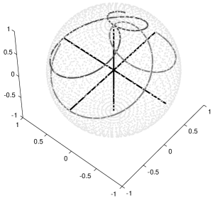
Finally, Fig. 2 shows plots of the trajectories of the spin vectors on (or near) the surface of a unit sphere, starting from an unentangled state with the first spin (light gray) along the ${\mathsf{x}}$-axis and the second (dark gray) along the ${\mathsf{z}}$-axis. The lengths of the spin vectors stayed very nearly at unity, implying that little entanglement was generated. The first spin executed a loop-de-loop up to the ${\mathsf{z}}$-axis, returned to the $-{\mathsf{x}}$-axis, and continued on in the general direction of the ${\mathsf{y}}$-axis, while the second swooped down towards the ${\mathsf{y}}$-axis, returned symmetrically to the ${\mathsf{z}}$-axis, and then ended half-way between the ${\mathsf{x}}$ & ${\mathsf{z}}$-axes. The complexity of the trajectories even in such a simple quantum system is impressive!

Refer to caption
Figure 2: Plot of the spin vector trajectories under the dipolar Hamiltonian starting from an unentangled state with the first spin (light gray) along the ${\mathsf{x}}$-axis and the second (dark gray) along the ${\mathsf{z}}$-axis. The length of the vectors stayed near unity, implying that the state remained largely unentangled throughout its acrobatics.

If we take the derivative of the spin bivector we get

$\displaystyle\partial_{t\,}{\boldsymbol{S}}(t)~{}=~{}$ $\displaystyle~{}2(-{\boldsymbol{H}}_{\mathsf{D\,}}\boldsymbol{\psi}{\boldsymbol{J}}){\boldsymbol{J}}\tilde{\boldsymbol{\psi}}\,+\,2\boldsymbol{\psi}{\boldsymbol{J}}(-{\boldsymbol{H}}_{\mathsf{D\,}}\boldsymbol{\psi}{\boldsymbol{J}})^{\scriptscriptstyle\!\sim\,}$
$\displaystyle~{}=~{}$ $\displaystyle~{}2\big{(}{\boldsymbol{H}}_{\mathsf{D\,}}\boldsymbol{\psi}\tilde{\boldsymbol{\psi}}\,-\,\boldsymbol{\psi}\tilde{\boldsymbol{\psi}}\,{\boldsymbol{H}}_{\mathsf{D}}\big{)}.$ (35)

Now ${\boldsymbol{H}}_{\mathsf{D}}$ is an MSTA 4-vector, while $\boldsymbol{\psi}\tilde{\boldsymbol{\psi}}$ is the sum of a 4-vector and a scalar. contains a 4-vector term as well as the scalar term. The commutator of two 4-vectors gives rise to terms of grade two, and it is this that gives rise to the interesting dynamics. If the state is separable we can write

$$2\,\bigl{\langle}\boldsymbol{\psi}\tilde{\boldsymbol{\psi}}\bigr{\rangle}_{4}~{}=~{}{\boldsymbol{\iota p}}^{1}{\boldsymbol{\iota\!q}}^{2},$$ (36)

where ${\boldsymbol{p}}$ and ${\boldsymbol{q}}$ are the single-particle spin vectors. In this case we have

$$\hskip 2.5pt\partial_{t\,}{\boldsymbol{S}}(t)~{}=~{}{\boldsymbol{H}}_{\mathsf{D}}\,{\boldsymbol{\iota p}}^{1}{\boldsymbol{\iota\!q}}^{2}-{\boldsymbol{\iota p}}^{1}{\boldsymbol{\iota\!q}}^{2}{\boldsymbol{H}}_{\mathsf{D}}\,.$$ (37)

For our Hamiltonian the general relation for commutators of tensor products of three-dimensional bivectors,

$\displaystyle\big{(}{\boldsymbol{A}}^{1}{\boldsymbol{B}}^{2}\big{)}\times\big{(}{\boldsymbol{X}}^{1}{\boldsymbol{Y}}^{2}\big{)}~{}\equiv~{}$ $\displaystyle~{}\mathchoice{\textstyle\frac{1}{2}}{\frac{1}{2}}{\frac{1}{2}}{\frac{1}{2}}\big{(}{\boldsymbol{A}}^{1}{\boldsymbol{B}}^{2}\big{)}\big{(}{\boldsymbol{X}}^{1}{\boldsymbol{Y}}^{2}\big{)}-\mathchoice{\textstyle\frac{1}{2}}{\frac{1}{2}}{\frac{1}{2}}{\frac{1}{2}}\big{(}{\boldsymbol{X}}^{1}{\boldsymbol{Y}}^{2}\big{)}\big{(}{\boldsymbol{A}}^{1}{\boldsymbol{B}}^{2}\big{)}$
$\displaystyle~{}=~{}$ $\displaystyle~{}{\boldsymbol{A}}\!\cdot\!{\boldsymbol{X}}\,\big{(}{\boldsymbol{B}}\times{\boldsymbol{Y}}\big{)}^{2}+{\boldsymbol{B}}\!\cdot\!{\boldsymbol{Y}}\,\big{(}{\boldsymbol{A}}\times{\boldsymbol{X}}\big{)}^{1}~{},$ (38)

enables us to reduce this to

$$\partial_{t\,}{\boldsymbol{S}}(t)\,=\,\frac{d}{2}\,({\boldsymbol{p}}\wedge{\boldsymbol{q}})^{1\!}-\frac{d}{2}\,({\boldsymbol{p}}\wedge{\boldsymbol{q}})^{2\!}+\frac{3d}{2}\,\boldsymbol{\sigma}_{\!3}\!\cdot\!{\boldsymbol{q}}\,(\boldsymbol{\sigma}_{\!3\!}\wedge{\boldsymbol{p}})^{1}+\frac{3d}{2}\,\boldsymbol{\sigma}_{\!3}\!\cdot\!{\boldsymbol{p}}\,(\boldsymbol{\sigma}_{\!3\!}\wedge{\boldsymbol{q}})^{2},\!\!\!$$ (39)

and we have recovered exactly the classical equation of motion for two dipolar-coupled spins. Of course, separability is not preserved in the case of quantum spins, due to differences in the higher derivatives. This allows the spin vectors to change their lengths (as the degree of entanglement varies), which cannot happen classically.

4 Lagrangian Analysis

Lagrangian methods play a central role in finding equations of motion for constrained systems such as rigid bodies in classical mechanics. Via Noether’s theorem, they also permit one to identify constants of the motion such as the total angular momentum, which provide insights into their long-term dynamics. Since quantum dynamics typically exhibit many more symmetries than classical, an extension of Lagrangian methods to multispin systems is highly desirable. This type of analysis is somewhat underutilized in traditional quantum treatments, as it sits somewhere between classical Lagrangian analysis and quantum operator techniques.

4.1 Single-Particle Systems

As a starting point, consider a single spin-1/2 particle interacting with an applied magnetic field described by the bivector ${\boldsymbol{B}}$. The Lagrangian for this is

$$L~{}=~{}\left\langle\dot{\boldsymbol{\psi}}\,\boldsymbol{\iota}\!\boldsymbol{\sigma}_{\!3}\,\tilde{\boldsymbol{\psi}}\,-\,\gamma{\boldsymbol{B}}\,\boldsymbol{\psi}\,\boldsymbol{\iota}\!\boldsymbol{\sigma}_{\!3}\,\tilde{\boldsymbol{\psi}}\right\rangle~{}.$$ (40)

Substituting this into the Euler-Lagrange equations

$$\frac{{\mathrm{d}}}{{\mathrm{d}}t}\left(\frac{\partial L}{\partial\dot{\boldsymbol{\psi}}}\right)\,=~{}\frac{\partial L}{\partial\boldsymbol{\psi}}$$ (41)

yields

$$\frac{{\mathrm{d}}}{{\mathrm{d}}t}\bigl{(}\boldsymbol{\iota}\!\boldsymbol{\sigma}_{\!3}\,\tilde{\boldsymbol{\psi}}\bigr{)}~{}=~{}\bigl{(}\dot{\boldsymbol{\psi}}\,\boldsymbol{\iota}\!\boldsymbol{\sigma}_{\!3}\bigr{)}^{\scriptscriptstyle\sim}\,-\,\gamma\bigl{(}\boldsymbol{\iota}\!\boldsymbol{\sigma}_{\!3}\,\tilde{\boldsymbol{\psi}}\,{\boldsymbol{B}}\bigr{)}\,-\,\gamma\bigl{(}{\boldsymbol{B}}\,\boldsymbol{\psi}\,\boldsymbol{\iota}\!\boldsymbol{\sigma}_{\!3}\bigr{)}^{\scriptscriptstyle\sim}~{}.$$ (42)

This simplifies readily to Schrödinger’s equation for the system:

$$\dot{\boldsymbol{\psi}}~{}=~{}\gamma{\boldsymbol{B}}\,\boldsymbol{\psi}.$$ (43)

This prototype can be used to build more realistic semi-classical models of spin, including relativistic effects [7]. A feature of this Lagrangian, which is typical for spin-$1/2$ systems, is that it is first order in $\dot{\boldsymbol{\psi}}$. For such systems one frequently finds that $L=0$ for paths satisfying the equations of motion.

4.2 Two-Particle Interactions

Of greater relevance here is the two-particle equation (17). This can be obtained from the Lagrangian

$$L(\boldsymbol{\psi},\dot{\boldsymbol{\psi}})~{}\equiv~{}2\left\langle\dot{\boldsymbol{\psi}}\,{\boldsymbol{J}}\,\tilde{\boldsymbol{\psi}}\,-\,{\boldsymbol{H}}_{\mathsf{D}}\,\boldsymbol{\psi}\,{\boldsymbol{E}}\,\tilde{\boldsymbol{\psi}}\right\rangle~{}.$$ (44)

The first term here can be viewed as the kinetic energy, and the second term as the potential energy. The latter term couples entirely through the 4-vector part of $\boldsymbol{\psi}\,{\boldsymbol{E}}\,\tilde{\boldsymbol{\psi}}$. Some insight into the nature of this system can be obtained by parameterizing the wavefunction as

$$\boldsymbol{\psi}~{}=~{}\boldsymbol{\upsilon}^{1}\boldsymbol{\zeta}^{2}(\cos(\theta/2)\boldsymbol{E}+\sin(\theta/2)\boldsymbol{\iota}\!\boldsymbol{\sigma}_{\!2}^{1}\boldsymbol{\iota}\!\boldsymbol{\sigma}_{\!2}^{2}\boldsymbol{J}){\boldsymbol{e}}^{\,\alpha{\boldsymbol{J}}}.$$ (45)

Here $\boldsymbol{\upsilon}$ and $\boldsymbol{\zeta}$ are single-particle spinors, $\theta$ measures the entanglement and $\alpha$ is an overall phase factor. In total this parameterization has 10 degrees of freedom, so 2 must be redundant. One of these is in the separate magnitudes of $\boldsymbol{\upsilon}$ and $\boldsymbol{\zeta}$, since only their product is involved in $\boldsymbol{\psi}$. The second redundant parameter is in the separate single-particle phases, since under the simultaneous transformation

$$\boldsymbol{\upsilon}\mapsto\boldsymbol{\upsilon}\,{\boldsymbol{e}}^{-\beta\boldsymbol{\iota}\!\boldsymbol{\sigma}_{\!3}},\quad\boldsymbol{\zeta}\mapsto\boldsymbol{\zeta}\,{\boldsymbol{e}}^{\beta\boldsymbol{\iota}\!\boldsymbol{\sigma}_{\!3}},$$ (46)

we see that $\boldsymbol{\psi}$ is unchanged. Despite this redundancy, the parameterization is extremely useful, as becomes clear when we write the kinetic term as

$$2\left\langle\dot{\boldsymbol{\psi}}\,{\boldsymbol{J}}\,\tilde{\boldsymbol{\psi}}\right\rangle~{}=~{}\cos(\theta)\bigl{\langle}\dot{\boldsymbol{\zeta}}\boldsymbol{\iota}\!\boldsymbol{\sigma}_{\!3}\tilde{\boldsymbol{\zeta}}\,(\boldsymbol{\upsilon}\tilde{\boldsymbol{\upsilon}})+\dot{\boldsymbol{\upsilon}}\boldsymbol{\iota}\!\boldsymbol{\sigma}_{\!3}\tilde{\boldsymbol{\upsilon}}\,(\boldsymbol{\zeta}\tilde{\boldsymbol{\zeta}})\bigr{\rangle}\,.$$ (47)

This would reproduce the classical dynamics of two magnetic dipoles, were it not for the factor of $\cos(\theta)$. We also see that there is no derivative term for $\theta$, so the Euler-Lagrange equation for the entanglement measure produces a simple algebraic equation.

The potential term in the Lagrangian can similarly be written

$\displaystyle-2\left\langle{\boldsymbol{H}}_{\mathsf{D}}\,\boldsymbol{\psi}\,{\boldsymbol{E}}\,\tilde{\boldsymbol{\psi}}\right\rangle~{}=~{}$ $\displaystyle-\left\langle{\boldsymbol{H}}_{\mathsf{D}}\,(\boldsymbol{\zeta}\boldsymbol{\iota}\!\boldsymbol{\sigma}_{\!3}\tilde{\boldsymbol{\zeta}})^{1}(\boldsymbol{\upsilon}\boldsymbol{\iota}\!\boldsymbol{\sigma}_{\!3}\tilde{\boldsymbol{\upsilon}})^{2}\right\rangle$
$\displaystyle+\,\sin(\theta)\left\langle{\boldsymbol{H}}_{\mathsf{D}}\,\boldsymbol{\zeta}^{1}\boldsymbol{\upsilon}^{2}\bigl{(}\boldsymbol{\iota}\!\boldsymbol{\sigma}_{\!1}^{1}\boldsymbol{\iota}\!\boldsymbol{\sigma}_{\!2}^{2}+\boldsymbol{\iota}\!\boldsymbol{\sigma}_{\!2}^{1}\boldsymbol{\iota}\!\boldsymbol{\sigma}_{\!1}^{2}\bigr{)}\tilde{\boldsymbol{\zeta}}^{1}\tilde{\boldsymbol{\upsilon}}^{2}\right\rangle.$ (48)

Again, it is the entanglement factor that adds the quantum effects. If we set $\theta=0$ in the Lagrangian then the equations of motion reduce to precisely those for a pair of classical dipoles. It is the presence of $\theta$ in the Lagrangian, which is forced upon us by the nature of multiparticle Hilbert space, that makes the system truly quantum mechanical.

4.3 Symmetries and Noether’s theorem

Symmetries of the Lagrangian give rise to conserved quantities via Noether’s theorem. Let $\boldsymbol{\psi}^{\prime}=\boldsymbol{\psi}^{\prime}(\boldsymbol{\psi},\alpha)$ be a differentiable transformation of the spinor $\boldsymbol{\psi}$ controlled by a single scalar $\alpha$, and satisfying $\boldsymbol{\psi}^{\prime}(\boldsymbol{\psi},0)=\boldsymbol{\psi}$. If we define the transformed Lagrangian as

$$L^{\prime}(\boldsymbol{\psi},\dot{\boldsymbol{\psi}})~{}\equiv~{}L(\boldsymbol{\psi}^{\prime},\smash{\dot{\boldsymbol{\psi}}}^{\prime})~{},$$ (49)

we find (using the Euler-Lagrange equations) that

$$\left.\frac{\partial L^{\prime}}{\partial\alpha}\right|_{\alpha=0}~{}=~{}\frac{{\mathrm{d}}}{{\mathrm{d}}t}\,\left\langle\left.\frac{\partial\boldsymbol{\psi}^{\prime}}{\partial\alpha}\right|_{\alpha=0}\,\frac{\partial L}{\partial\dot{\boldsymbol{\psi}}}\right\rangle~{}=~{}2\frac{{\mathrm{d}}}{{\mathrm{d}}t}\,\left\langle\boldsymbol{\phi}\,{\boldsymbol{J}}\,\tilde{\boldsymbol{\psi}}\right\rangle~{},$$ (50)

where $\boldsymbol{\phi}\equiv\partial\boldsymbol{\psi}^{\prime}\!/\partial\alpha|_{\alpha=0\,}$. If $L^{\prime}$ is independent of $\alpha$ our transformation defines a symmetry of the Lagrangian, and gives rise to a conjugate conserved quantity.

As a simple example, take the invariance of $L$ under changes of phase:

$$\boldsymbol{\psi}^{\prime}~{}=~{}\boldsymbol{\psi}\,{\boldsymbol{e}}^{\,\alpha{\boldsymbol{J}}}~{}\implies~{}\;\boldsymbol{\phi}~{}=~{}\boldsymbol{\psi}\,{\boldsymbol{J}}~{}.$$ (51)

It is easily seen that this is a symmetry of the Lagrangian, and that the conjugate conserved quantity is $-2\langle\boldsymbol{\psi}\tilde{\boldsymbol{\psi}}\rangle$, telling us that the magnitude of $\boldsymbol{\psi}$ is constant.

Phase changes are something of an exception in that they involve operation on $\boldsymbol{\psi}$ from the right. Operation from the left by a term of the form $\boldsymbol{\exp}(\alpha{\boldsymbol{P}})$ will always generate a symmetry provided ${\boldsymbol{P}}$ commutes with the Hamiltonian. The prime example in this case is the Hamiltonian ${\boldsymbol{H}}_{\mathsf{D}}$ itself. The symmetry this generates corresponds is time translation, as defined by the ${\boldsymbol{\exp}}(-\boldsymbol{j}{\boldsymbol{H}}_{\mathsf{D\,}}t)$ and the conjugate conserved quantity is the total internal energy. Another important symmetry generator is provided by $\boldsymbol{\iota}\!\boldsymbol{\sigma}_{\!3}^{1}+\boldsymbol{\iota}\!\boldsymbol{\sigma}_{\!3}^{2}$, which generates rotation of both spins about the ${\mathsf{z}}$-axis at equal rates. (Recall that this axis is defined by the inter-dipole vector.) This bivector commutes with the Hamiltonian since

$${\boldsymbol{H}}_{\mathsf{D}}\,\big{(}\boldsymbol{\iota}\!\boldsymbol{\sigma}_{\!3}^{1}+\boldsymbol{\iota}\!\boldsymbol{\sigma}_{\!3}^{2}\big{)}~{}=~{}-\frac{d}{4}\,\big{(}\boldsymbol{\iota}\!\boldsymbol{\sigma}_{\!3}^{1}+\boldsymbol{\iota}\!\boldsymbol{\sigma}_{\!3}^{2}\big{)}~{}=~{}\big{(}\boldsymbol{\iota}\!\boldsymbol{\sigma}_{\!3}^{1}+\boldsymbol{\iota}\!\boldsymbol{\sigma}_{\!3}^{2}\big{)}\,{\boldsymbol{H}}_{\mathsf{D}}~{},$$ (52)

and the conjugate conserved quantity is

$$(\boldsymbol{\iota}\!\boldsymbol{\sigma}_{\!3}^{1}+\boldsymbol{\iota}\!\boldsymbol{\sigma}_{\!3}^{2})\!\cdot\!(2\boldsymbol{\psi}\,{\boldsymbol{J}}\,\tilde{\boldsymbol{\psi}})=(\boldsymbol{\iota}\!\boldsymbol{\sigma}_{\!3}^{1}+\boldsymbol{\iota}\!\boldsymbol{\sigma}_{\!3}^{2})\!\cdot\!\boldsymbol{S},$$ (53)

which gives the total angular momentum about the ${\mathsf{z}}$-axis.

Yet another symmetry generator is found by considering the operator for the magnitude of the total angular momentum, namely

$$\begin{split}&~{}\bigl{(}\boldsymbol{\iota}\!\boldsymbol{\sigma}_{\!1}^{1}+\boldsymbol{\iota}\!\boldsymbol{\sigma}_{\!1}^{2}\bigr{)}^{2}\,+\,\bigl{(}\boldsymbol{\iota}\!\boldsymbol{\sigma}_{\!2}^{1}+\boldsymbol{\iota}\!\boldsymbol{\sigma}_{\!2}^{2}\bigr{)}^{2}\,+\,\bigl{(}\boldsymbol{\iota}\!\boldsymbol{\sigma}_{\!3}^{1}+\boldsymbol{\iota}\!\boldsymbol{\sigma}_{\!3}^{2}\bigr{)}^{2}\\ =~{}&~{}2\,\bigl{(}\boldsymbol{\iota}\!\boldsymbol{\sigma}_{\!1}^{1}\boldsymbol{\iota}\!\boldsymbol{\sigma}_{\!1}^{2}\,+\,\boldsymbol{\iota}\!\boldsymbol{\sigma}_{\!2}^{1}\boldsymbol{\iota}\!\boldsymbol{\sigma}_{\!2}^{2}\,+\,\boldsymbol{\iota}\!\boldsymbol{\sigma}_{\!3}^{1}\boldsymbol{\iota}\!\boldsymbol{\sigma}_{\!3}^{2}\,-\,3\bigr{)}~{}=~{}-4\,\big{(}1\,+\,\boldsymbol{\Pi}\big{)}~{}.\end{split}$$ (54)

The new generator here is $\boldsymbol{j}\boldsymbol{\Pi}$, which generates a continuous version of particle interchange, and is a symmetry of $L$. The conjugate conserved quantity is $\langle\boldsymbol{\Pi}\,\boldsymbol{\psi}\tilde{\boldsymbol{\psi}}\rangle$. Rather confusingly, this is not the same as the total magnitude $\langle\boldsymbol{S}\boldsymbol{S}\rangle$, which is not conserved in the quantum case (though it is conserved classically where the spin vectors have fixed length).

Together with phase invariance, we have now found a total of four physically relevant constants of motion for the two-spin dipolar Hamiltonian ${\boldsymbol{H}}_{\mathsf{D\,}}$. Are there any more? Clearly any linear combination of constants of motion is again a constant of motion, so this can only be answered in the sense of finding a complete basis for the subspace spanned by the constants of motion in the $16$-dimensional space of all observables. The dimension of this subspace can be determined by considering the eigenstructure of ${\boldsymbol{H}}_{\mathsf{D}}$ again (Eq. 24). Clearly the observable which measures the amount of a state in any one eigenspinor is a constant of the motion, and more generally, each eigenvalue gives rise to $\delta^{2}$ constants of the motion where $\delta$ is its degeneracy. Since ${\boldsymbol{H}}_{\mathsf{D}}$ has one two-fold degenerate eigenvalue, the constants of motion must span a subspace of dimension $1+1+2^{2}=6$, and we are therefore just two short! It is quite easy to see, however, that the so-called (in NMR) double quantum coherences

$$\boldsymbol{\iota}\!\boldsymbol{\sigma}_{\!1}^{1}\boldsymbol{\iota}\!\boldsymbol{\sigma}_{\!1}^{2}\,-\,\boldsymbol{\iota}\!\boldsymbol{\sigma}_{\!2}^{1}\boldsymbol{\iota}\!\boldsymbol{\sigma}_{\!2}^{2}\quad\text{and}\quad\boldsymbol{\iota}\!\boldsymbol{\sigma}_{\!1}^{1}\boldsymbol{\iota}\!\boldsymbol{\sigma}_{\!2}^{2}\,+\,\boldsymbol{\iota}\!\boldsymbol{\sigma}_{\!2}^{1}\boldsymbol{\iota}\!\boldsymbol{\sigma}_{\!1}^{2}$$ (55)

commute with ${\boldsymbol{H}}_{\mathsf{D}}$ and generate two new independent symmetries. The physical interpretation of these symmetries is far from simple as they again involve the geometry of the 4-vector $\langle\boldsymbol{\psi}\,\tilde{\boldsymbol{\psi}}\rangle_{4}$. Because the product of any two constants of motion is again a constant of motion, the constants of motion constitute a subalgebra (of the even subalgebra) of the MSTA. This makes it possible to form large numbers of new constants in order to find those with the simplest physical or geometric interpretations.

5 The Density Operator

For a single-particle normalized pure state the quantum density operator is

$$\hat{\rho}~{}=~{}|\,\psi\,\rangle\langle\,\psi\,|~{}=~{}\mathchoice{\textstyle\frac{1}{2}}{\frac{1}{2}}{\frac{1}{2}}{\frac{1}{2}}\,\big{(}\hat{I}+{\textstyle\sum}_{k=1\,}^{3}\,p_{k}\,\hat{\sigma}_{k}\big{)}\,,$$ (56)

where $\hat{I}$ is the identity operator on a two-dimensional Hilbert space, and

$$p_{k}~{}=~{}\langle\,\psi\,|\,\hat{\sigma}_{k}\,|\,\psi\,\rangle\,.$$ (57)

The MSTA equivalent of this is simply

$$\boldsymbol{\psi}\,{\boldsymbol{Z}}_{+\,}\tilde{\boldsymbol{\psi}}~{}=~{}\mathchoice{\textstyle\frac{1}{2}}{\frac{1}{2}}{\frac{1}{2}}{\frac{1}{2}}(1+{\boldsymbol{p}})~{},$$ (58)

where ${\boldsymbol{Z}}_{\pm}\equiv\mathchoice{\textstyle\frac{1}{2}}{\frac{1}{2}}{\frac{1}{2}}{\frac{1}{2}}(1\pm\boldsymbol{\sigma}_{\!3})$ are idempotents and ${\boldsymbol{p}}={\boldsymbol{\psi}}\,\boldsymbol{\sigma}_{\!3}\,{\boldsymbol{\tilde{\psi}}}$ is known as the Bloch or spin polarization vector.

The most straightforward extension of this to the multiparticle case replaces the idempotent by the product of those for all the $n$ distinguishable spins: ${\boldsymbol{Z}}_{+}\equiv{\boldsymbol{Z}}_{+}^{1}\cdots{\boldsymbol{Z}}_{+}^{n}$. This has the added benefit of enabling one to absorb all the $\boldsymbol{\sigma}_{\!3}^{a}$ vectors from ${\boldsymbol{E}}$ into ${\boldsymbol{Z}}_{+\,}$, thereby converting ${\boldsymbol{E}}$ into a pseudoscalar correlator,

$${\boldsymbol{C}}~{}=~{}\mathchoice{\textstyle\frac{1}{2}}{\frac{1}{2}}{\frac{1}{2}}{\frac{1}{2}}(1-\boldsymbol{\iota}^{1}\boldsymbol{\iota}^{2})\cdots\mathchoice{\textstyle\frac{1}{2}}{\frac{1}{2}}{\frac{1}{2}}{\frac{1}{2}}(1-\boldsymbol{\iota}^{1}\boldsymbol{\iota}^{n})~{}.$$ (59)

This commutes with the entire even MSTA subalgebra, and allows one to identify all the pseudoscalars $\boldsymbol{\iota}^{a}$, wherever they occur, with a single global imaginary as in conventional quantum mechancs. This faithfully reproduces all standard results, but the idempotent ${\boldsymbol{Z}}_{+}^{1}\cdots{\boldsymbol{Z}}_{+}^{n}$ does not live in the even subalgebra, and hence mixes up the grades of entities which otherwise would have a simpler geometric meaning. In the following we propose for the first time a formulation of the density operator within the even subalgebra of the MSTA.

The key is to observe that both ${\boldsymbol{Z}}_{+}^{1}\cdots{\boldsymbol{Z}}_{+}^{n}$ and ${\boldsymbol{E}}+{\boldsymbol{J}}$ contain all $2^{n}$ possible products of the $\boldsymbol{\sigma}_{\!3}^{a}$ ($a=1,\ldots,n$). It follows that the even MSTA density operator

$${\boldsymbol{\rho}}_{*}~{}\equiv~{}2^{n-1}\,\boldsymbol{\psi}\,\big{(}{\boldsymbol{E}}\,+\,{\boldsymbol{J}}\big{)}\,\tilde{\boldsymbol{\psi}}$$ (60)

includes the same complete set of commuting observables as does the usual definition (modulo pseudoscalar factors). The normalization of $2^{n-1}$ is chosen so that the scalar part $\langle{\boldsymbol{\rho}}_{*}\rangle=1$. This is more natural when using geometric algebra than the usual factor of $1/2$, which ensures that the trace of the identity state ${\boldsymbol{I}}/2^{n}$ is unity. The density operator of a mixed state is simply the statistical average of these observables as usual: ${\boldsymbol{\rho}}_{*}\equiv\overline{\boldsymbol{\psi}({\boldsymbol{E}}\,+\,{\boldsymbol{J}})\tilde{\boldsymbol{\psi}}}$ [10, 11].

There is a problem with the even MSTA version, however, which is that $\boldsymbol{\psi}\,\boldsymbol{J}\tilde{\boldsymbol{\psi}}$ is anti-Hermitian (under reversion), whereas the usual density operator is Hermitian. In addition, up to now we have only applied the propagator to spinors, where the complex structure is given by right-multiplication with $\boldsymbol{J}$. Such a representation is not appropriate for density operators, because to apply it we would have to decompose our density operator into a sum over an ensemble of known pure states, apply the propagator to each state’s spinor, and then rebuild the density operator from the transformed ensemble. This is clearly undesirable, so we should re-think the role of the imaginary in the propagator for the density operator.

To do this, we must first understand the role of $i$ in the propagator, where it appears multiplying the (Hermitian) Hamiltonian $\hat{H}$. The terms in $i\hat{H}$ involving odd numbers of particles have an immediate counterpart in the MSTA as products of odd numbers of bivectors. These exponentiate straightforwardly in the MSTA, and here the role of the imaginary as a pseudoscalar is clear. It is the terms in $i\hat{H}$ involving even numbers of particles which are the problem. When these are converted to products of even numbers of bivectors, a single factor of $i$ is left over. To see its effect we return to a pure state and consider

$$(\boldsymbol{j}\boldsymbol{\psi})\tilde{\boldsymbol{\psi}}~{}=~{}\boldsymbol{\psi}\,\boldsymbol{J}\tilde{\boldsymbol{\psi}}\quad\mbox{and}\quad(\boldsymbol{j}\boldsymbol{\psi})\boldsymbol{J}\tilde{\boldsymbol{\psi}}~{}=~{}-\boldsymbol{\psi}\,\tilde{\boldsymbol{\psi}}\,.$$ (61)

Thus we see that, applied to density operators (or any other observables), the imaginary unit interchanges even and odd terms (in their number of bivectors), in addition to squaring to $-1$.

It follows that the left-over factor of $i$ in the even terms converts them to odd terms, thereby ensuring that the Hamiltonian generates a compact group while at the same time labeling these terms to keep them separate from the original odd terms. This is quite different from other occurrences of the imaginary! A simple way to represent this in the even MSTA is to introduce a “formal” imaginary unit $j$, and to redefine the even MSTA density operator as

$${\boldsymbol{\rho}}~{}\equiv~{}{\boldsymbol{\rho}}_{+}\,-\,j\,{\boldsymbol{\rho}}_{-}$$ (62)

where ${\boldsymbol{\rho}}_{+}\equiv{\langle{\boldsymbol{\rho}}_{*}\rangle}_{0}+{\langle{\boldsymbol{\rho}}_{*}\rangle}_{4}+\cdots$ and ${\boldsymbol{\rho}}_{-}\equiv{\langle{\boldsymbol{\rho}}_{*}\rangle}_{2}+{\langle{\boldsymbol{\rho}}_{*}\rangle}_{8}+\cdots$. Then, provided any residual factors of the even MSTA operator $\boldsymbol{j}$ are replaced by $j$, everything works simply. In writing ${\boldsymbol{\rho}}$ in this way we have also recovered a more standard, Hermitian representation, which permits the mean expectation values of any observable $\boldsymbol{o}=\boldsymbol{o}_{+}+j\boldsymbol{o}_{-}$ to be computed by essentially the usual formula:

$$\langle\,\boldsymbol{o}\,{\boldsymbol{\rho}}\,\rangle_{0}~{}=~{}\langle\,(\boldsymbol{o}_{+}\,+\,j\,\boldsymbol{o}_{-})({\boldsymbol{\rho}}_{+}\,-\,j\,{\boldsymbol{\rho}}_{-})\,\rangle_{0}~{}=~{}\langle\,\boldsymbol{o}_{+\,}{\boldsymbol{\rho}}_{+}\,+\,\boldsymbol{o}_{-\,}{\boldsymbol{\rho}}_{-}\,\rangle_{0}~{}.$$ (63)

The geometric interpretation of this new imaginary operator $j$ will be further considered on a subsequent occasion.

5.1 An Example of Information Dynamics

We are now ready to see how things look to one spin when no information about the other(s) is available. Clearly this depends on the (unknown!) configuration of the other spin(s), and we expect that the “generic” case will result in a very complicated trajectory, which may also be incoherent in the sense that the length of the spin vector is not preserved. Somewhat surprisingly, the situation is simplified substantially by assuming that the spin of interest has an environment consisting of a great many others, whose dynamics are so complex that their spin vectors can be treated as completely random. Under these circumstances, neither the exact starting state of the environment, nor any subsequent change in it, will change the way our chosen spin (henceforth numbered $1$) sees it. As a result of this assumption and the linearity of quantum dynamics, we need only figure out how its basis states $\boldsymbol{\iota}\!\boldsymbol{\sigma}_{\!1}^{1},\boldsymbol{\iota}\!\boldsymbol{\sigma}_{\!2}^{1},\boldsymbol{\iota}\!\boldsymbol{\sigma}_{\!3}^{1}$ evolve in order to determine its evolution in general.

To see how the $\boldsymbol{\iota}\!\boldsymbol{\sigma}_{\!k}^{1}$ evolve, we return to the propagator of equation (21), which we now write in the form

$$\boldsymbol{\exp}\big{(}\!-\!j\,{\boldsymbol{H}}_{\mathsf{D\,}}t\big{)}~{}=~{}\boldsymbol{\exp}\big{(}\!-\!j\,\boldsymbol{\iota}\!\boldsymbol{\sigma}_{\!3}^{1}\boldsymbol{\iota}\!\boldsymbol{\sigma}_{\!3}^{2}\,3dt/4\big{)}\,\boldsymbol{\exp}\big{(}\!-\!j\,\boldsymbol{\Pi}\,dt/2\big{)}\,\boldsymbol{\exp}\big{(}j_{\,}dt/4\big{)}\,.$$ (64)

The phase term has no effect, and for the interchange term we find that

$\displaystyle{\boldsymbol{e}}^{-j\,\boldsymbol{\Pi}\,dt/2}\,\boldsymbol{\iota}\!\boldsymbol{\sigma}_{\!k}^{1}\,{\boldsymbol{e}}^{\,j\,\boldsymbol{\Pi}\,dt/2}~{}=~{}$ $\displaystyle~{}\cos^{2}(dt/2)\,\boldsymbol{\iota}\!\boldsymbol{\sigma}_{\!k}^{1}+\sin^{2}(dt/2)\,\boldsymbol{\iota}\!\boldsymbol{\sigma}_{\!k}^{2}$
$\displaystyle\qquad-\,j\,\sin(dt)\,\boldsymbol{\Pi}\times\boldsymbol{\iota}\!\boldsymbol{\sigma}_{\!k}^{1}\,.$ (65)

We then need to apply the term in $\boldsymbol{\exp}(j\,\boldsymbol{\iota}\!\boldsymbol{\sigma}_{\!3}^{1}\boldsymbol{\iota}\!\boldsymbol{\sigma}_{\!3}^{2}\,3dt/4)$. This commutes with $\boldsymbol{\Pi}$, so we only need to transform the separate bivectors. For the case of $k=3$ this final term has no effect, and we have

$\displaystyle{\boldsymbol{e}}^{-j_{\,}{\boldsymbol{H}}_{\mathsf{D\,}}t}\,\boldsymbol{\iota}\!\boldsymbol{\sigma}_{\!3}^{1}\,{\boldsymbol{e}}^{\,j_{\,}{\boldsymbol{H}}_{\mathsf{D\,}}t}~{}=~{}$ $\displaystyle~{}\mathchoice{\textstyle\frac{1}{2}}{\frac{1}{2}}{\frac{1}{2}}{\frac{1}{2}}\big{(}1+\cos(dt)\big{)}\boldsymbol{\iota}\!\boldsymbol{\sigma}_{\!3}^{1}\,+\,\mathchoice{\textstyle\frac{1}{2}}{\frac{1}{2}}{\frac{1}{2}}{\frac{1}{2}}\big{(}1-\cos(dt)\big{)}\boldsymbol{\iota}\!\boldsymbol{\sigma}_{\!3}^{2}$
$\displaystyle\qquad-\,j\,\sin(dt)\,\mathchoice{\textstyle\frac{1}{2}}{\frac{1}{2}}{\frac{1}{2}}{\frac{1}{2}}\big{(}\boldsymbol{\iota}\!\boldsymbol{\sigma}_{\!1}^{1}\boldsymbol{\iota}\!\boldsymbol{\sigma}_{\!2}^{2}-\boldsymbol{\iota}\!\boldsymbol{\sigma}_{\!2}^{1}\boldsymbol{\iota}\!\boldsymbol{\sigma}_{\!1}^{2}\big{)}.$ (66)

For $k=1,2$ we need the result

$${\boldsymbol{e}}^{-j_{\,}\boldsymbol{\iota}\!\boldsymbol{\sigma}_{\!3}^{1}\boldsymbol{\iota}\!\boldsymbol{\sigma}_{\!3}^{2}\,\phi/2\,}\boldsymbol{\iota}\!\boldsymbol{\sigma}_{\!2}^{1}\,{\boldsymbol{e}}^{\,j_{\,}\boldsymbol{\iota}\!\boldsymbol{\sigma}_{\!3}^{1}\boldsymbol{\iota}\!\boldsymbol{\sigma}_{\!3}^{2}\,\phi/2}~{}=~{}\cos(\phi)\,\boldsymbol{\iota}\!\boldsymbol{\sigma}_{\!2}^{1}-j\,\sin(\phi)\,\boldsymbol{\iota}\!\boldsymbol{\sigma}_{\!1}^{1}\boldsymbol{\iota}\!\boldsymbol{\sigma}_{\!3}^{2}\,.$$ (67)

Combining this with the preceding we see that

$\displaystyle{\boldsymbol{e}}^{-j_{\,}{\boldsymbol{H}}_{\mathsf{D\,}}t}\,\boldsymbol{\iota}\!\boldsymbol{\sigma}_{\!2}^{1}\,{\boldsymbol{e}}^{\,j_{\,}{\boldsymbol{H}}_{\mathsf{D\,}}t}~{}=~{}$ $\displaystyle\big{(}\!\cos(dt){\scriptstyle\,}\boldsymbol{\iota}\!\boldsymbol{\sigma}_{\!2}^{1}-\sin(dt){\scriptstyle\,}j\,\boldsymbol{\iota}\!\boldsymbol{\sigma}_{\!1}^{1}\boldsymbol{\iota}\!\boldsymbol{\sigma}_{\!3}^{2}\big{)}\cos(dt/2)$
$\displaystyle-\big{(}\!\cos(dt){\scriptstyle\,}j\,\boldsymbol{\iota}\!\boldsymbol{\sigma}_{\!3}^{1}\boldsymbol{\iota}\!\boldsymbol{\sigma}_{\!1}^{2}+\sin(dt){\scriptstyle\,}\boldsymbol{\iota}\!\boldsymbol{\sigma}_{\!2}^{2}\big{)}\sin(dt/2)\,,$ (68)

with a similar result holding for $\boldsymbol{\iota}\!\boldsymbol{\sigma}_{\!1}^{1}$.

As a simple model, suppose that our initial state is described by a known state of particle 1, encoded in the density operator ${\boldsymbol{\rho}}(0)=(1+{\boldsymbol{p}}(0))/2$, and with the state of the second spin taken to be totally random. To evolve the density matrix of particle 1 we write $\boldsymbol{\iota}\!{\boldsymbol{p}}(0)=\sum_{k\,}p_{k}\boldsymbol{\iota}\!\boldsymbol{\sigma}_{\!k}^{1}$ and evolve each term as above. We then project ${\boldsymbol{\rho}}(t)$ back into the first particle space (by throwing out any terms involving other spins) and reform the polarization vector. We then find that:

$${\boldsymbol{p}}(t)~{}=~{}\cos(dt)\cos(dt/2)\,\big{(}p_{1\,}\boldsymbol{\sigma}_{\!1}~{}+~{}p_{2\,}\boldsymbol{\sigma}_{\!2}\big{)}\,+\,\cos^{2}(dt/2)\,p_{3\,}\boldsymbol{\sigma}_{\!3}~{}.$$ (69)

Of course, the same result is obtained if everything is rotated to some other orientation, for example if the other spin is along ${\mathsf{x}}$ and ${\boldsymbol{p}}$ is replaced by the rotated spin vector.

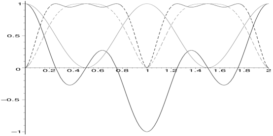
The von Neumann entropy of the spin, which measures how much information about its state has been lost to the environment, is given (in bits) by

$\displaystyle S_{\mathsf{vN}}~{}=~{}$ $\displaystyle-\mathchoice{\textstyle\frac{1}{2}}{\frac{1}{2}}{\frac{1}{2}}{\frac{1}{2}}(1+\|{\boldsymbol{p}}(t)\|)\log_{2}\big{(}(1+\|{\boldsymbol{p}}(t)\|)/2\big{)}$
$\displaystyle-\mathchoice{\textstyle\frac{1}{2}}{\frac{1}{2}}{\frac{1}{2}}{\frac{1}{2}}(1-\|{\boldsymbol{p}}(t)\|)\log_{2}\big{(}(1-\|{\boldsymbol{p}}(t)\|)/2\big{)}~{}.$ (70)

The signed lengths of the spin polarization vectors and the corresponding von Neumann entropies are plotted in Fig. 3 for a second spin in a random state and displaced from the first in directions parallel and perpendicular to its polarization vector.

Refer to caption
Figure 3: Dipolar “tides” (in units of $1/d$) exerted on a spin’s polarization vector by its interactions with a random ensemble of other spins all located in a circular “orbit” about its equator (light gray line), or at a fixed distance above its poles (dark gray line), along with the corresponding von Neumann entropies (dashed lines).

5.2 Towards Quantum Complexity and Decoherence

Our applications of geometric algebra to the problem of two dipole-coupled spins has illustrated how quantum interactions allow qubits to exchange information (states), in the process passing through an entangled state in which no information on either is directly accessible. We have also seen how information on the state of a qubit can be lost through its interactions with an environment, although the Poncaire recurrence times for the simple one-qubit environments we have considered are short enough to allow us to also see the underlying periodic behavior. This constitutes the simplest case of an old and venerable problem in solid-state NMR spectroscopy, which is to predict the spectral line-shape (decay envelope) of a macroscopic system of dipole-coupled spins such as calcium fluoride [1, 5, 19]. Here an exact treatment is out of the question, since the analytic evaluation of even the three-spin propagator is a reasonably challenging (though solvable) problem. Nevertheless, we believe the insights provided by geometric algebra, particularly into the constants of the motion, offer the hope of further progress.

More generally, quantum mechanical explanations of apparently irreversible processes are becoming increasingly important in many fields [22], and further have the potential to finally clarify in just what sense classical mechanics can be regarded as a limiting case of quantum mechanics [9]. These problems typically involve the spatial degrees of freedom, and hence are truly infinite dimensional. Most of what is known about decoherence in such systems therefore comes from the analysis of simple and highly tractable environmental models such as a bath of spins or harmonic oscillators. Because of its potential to provide global insights into the full spacetime structure of such models, we expect that the MSTA will also come to play an enabling role in our understanding of the quantum mechanical mechanisms operative in decoherence.


Acknowledgements

TFH thanks Prof. David Cory of MIT for useful discussions on NMR, and ARO grant DAAG55-97-1-0342 & DARPA grant MDA972-01-1-0003 for financial support. CJLD is supported by the EPSRC.

References

  • [1] A. Abragam, Principles of Nuclear Magnetism, Oxford Univ. Press, Oxford, UK, 1961.
  • [2] W. E. Baylis, ed., Clifford (Geometric) Algebras, with Applications in Physics, Mathematics, and Engineering, Birkhauser, Boston MA, 1996.
  • [3] C. H. Bennett and D. P. DiVincenzo, Quantum information and computation, Nature, 404 (2000), pp. 247–255.
  • [4] C. H. Bennett and R. Landauer, The fundamental physical limits of computation, Sci. Am., 253 (1985), pp. 38–46.
  • [5] B. Cowan, Nuclear Magnetic Resonance and Relaxation, Cambridge Univ. Press, Cambridge, UK, 1997.
  • [6] C. J. L. Doran, A. N. Lasenby, and S. F. Gull, States and operators in the spacetime algebra, Found. Phys., 23 (1993), pp. 1239–1264.
  • [7] C. J. L. Doran, A. N. Lasenby, S. F. Gull, S. S. Somaroo, and A. D. Challinor, Spacetime algebra and electron physics, in Advances in Imaging and Electron Physics, P. Hawkes, ed., Academic Press, Englewood Cliffs, NJ, 1996, pp. 271–386.
  • [8] R. P. Feynman, R. W. Allen, and A. J. G. Hey, eds., Feynman Lectures on Computation, Perseus Books, 2000.
  • [9] D. Giulini, E. Joos, C. Kiefer, J. Kupsch, I. Stamatescu, and H. D. Zeh, Decoherence and the Appearance of a Classical World in Quantum Theory, Springer-Verlag, Berlin, FRG, 1996.
  • [10] T. F. Havel, D. G. Cory, S. S. Somaroo, and C. Tseng, Geometric algebra methods in quantum information processing by NMR spectroscopy, in Advances in Geometric Algebra with Applications, Birkhauser, Boston, MA, USA, 2000.
  • [11] T. F. Havel and C. Doran, Geometric algebra in quantum information processing, 2001. Contemporary Math., in press (see LANL preprint quant-ph/0004031).
  • [12] D. Hestenes, Space-Time Algebra, Gordon and Breach, New York, NY, 1966.
  • [13] D. Hestenes, New Foundations for Classical Mechanics (2nd ed.), Kluwer Academic Pub., 1999.
  • [14] M. A. Nielsen and I. L. Chuang, Quantum Computation and Quantum Information, Cambridge Univ. Press, 2000.
  • [15] J. P. Paz and W. H. Zurek, Environment-induced decoherence and the transition from quantum to classical, in Coherent Atomic Matter Waves, R. Kaiser, ed., Springer-Verlag, 2001.
  • [16] I. Percival, Quantum State Diffusion, Cambridge Univ. Press, U.K., 1998.
  • [17] A. Peres, Quantum Theory: Concepts and Methods, Kluwer Academic Pub., Amsterdam, NL, 1993.
  • [18] C. P. Slichter, Principles of Magnetic Resonance (3rd. ed.), Springer-Verlag, Berlin, Germany, 1990.
  • [19] D. K. Sodickson and J. S. Waugh, Spin diffusion on a lattice: Classical simulations and spin coherent states, Phys. Rev. B, 52 (1995), pp. 6467–6469.
  • [20] S. Somaroo, A. Lasenby, and C. Doran, Geometric algebra and the causal approach to multiparticle quantum mechanics, J. Math. Phys., 40 (1999), pp. 3327–3340.
  • [21] S. S. Somaroo, D. G. Cory, and T. F. Havel, Expressing the operations of quantum computing in multiparticle geometric algebra, Phys. Lett. A, 240 (1998), pp. 1–7.
  • [22] U. Weiss, Quantum Dissipative Systems (2nd Ed.), World Scientific, 1999.
  • [23] C. P. Williams and S. H. Clearwater, Ultimate Zero and One: Computing at the Quantum Frontier, Copernicus Books, 1999.