Bound states in point-interaction star graphs

a) Department of Theoretical Physics, Nuclear Physics Institute,
e)xAcademy of Sciences, 25068 Řež, Czechia
b) Doppler Institute, Czech Technical University, Břehová 7,
e)x11519 Prague, Czechia
c) Faculty of Mathematics and Physics, Charles University,
e)xV Holešovičkách 2, 18000 Prague, Czechia
e)xexner@ujf.cas.cz, nemcova@ujf.cas.cz

We discuss the discrete spectrum of the Hamiltonian describing a two-dimensional quantum particle interacting with an infinite family of point interactions. We suppose that the latter are arranged into a star-shaped graph with $N$ arms and a fixed spacing between the interaction sites. We prove that the essential spectrum of this system is the same as that of the infinite straight “polymer”, but in addition there are isolated eigenvalues unless $N=2$ and the graph is a straight line. We also show that the system has many strongly bound states if at least one of the angles between the star arms is small enough. Examples of eigenfunctions and eigenvalues are computed numerically.

1 Introduction

Graph-type systems are used in quantum mechanics for a long time [RS], but only in the last decade they became a subject of an intense interest – cf. [KS] and references therein. Among various graph geometries, star graphs were investigated from different point of view. Recall, for instance, a natural generalization of the weak-coupling analysis for one-dimensional Schrödinger operators [E1], signatures of quantum chaos found recently in stars with finite nonequal arms [BBK], etc.

From the mathematical point of view Schrödinger operators on graphs are easy to deal with, because they represent systems of Sturm-Liouville ODE’s coupled through boundary conditions at the graph vertices. This is due to the assumption that the configuration space of the system is just the graph. From the physical point of view, this is certainly an idealization. One of the most common applications of graph models is a description of various mesoscopic systems like quantum wires, arrays of quantum dots, etc. In reality their boundaries are finite potential steps, and therefore the particle can move away from the prescribed area, even if not too far because the exterior of such a graph is a classically forbidden region.

There are various ways how to model such “leaky” graphs. One can use Schrödinger operator with a Dirac measure potential supported by the graph – see [BT, EI] and references therein. Here we consider another, in a sense more singular model where the graph is represented by a family of two-dimensional point interactions. Its advantage is that such a model is solvable because (the discrete part of) the spectral analysis is reduced essentially to an algebraic problem. Two-dimensional point-interaction Hamiltonians were studied by various authors – references can be found in the monograph [AGHH]. Nevertheless, relations between spectral properties of such operators and the geometry of the set of point-interaction sites did not attract much attention. Here we are going to fill this gap partly by discussing an example of a point-interaction star graph.

The model is described in the following section. Next, in Section 3, we show that the essential spectrum is given by the structure of each graph arm at large distances and thus it coincides with that of an infinite straight “polymer” [AGHH, Sec. III.4]. More surprising is the fact that a star graph has a nonempty discrete spectrum, with the exception of the trivial case when the graph is a straight line. This is proved in Section 4 where we also show that there are geometries which give rise to numerous strongly bound states. In the final section we present numerically computed examples showing eigenvalues and eigenfunctions for various graph configurations. Of course, the discrete spectrum is not the only interesting aspect of these Hamiltonians. One can ask about the scattering, perturbations coming either from changes in the geometry or from external fields, etc. We leave this questions to a future publication.

2 Formulation of the problem

For a given integer $N\geq 2$, consider an $(N\!-\!1)$-tuple of positive numbers $\beta:=(\beta_{1},\ldots,\beta_{N-1})$ such that $\sum_{j=1}^{N-1}\beta_{j}<2\pi$ and denote $\vartheta_{j}:=\sum_{i=1}^{j}\beta_{i}$ and $\vartheta_{0}:=0$. Then one can define the set

$$Y=\bigcup_{j=0}^{N-1}\{(nl\cos(\vartheta_{j}),nl\sin(\vartheta_{j}))\}_{n\in\mathbb{N}}\cup(0,0),$$

where $l>0$ is a given distance which has the meaning of the spacing of points at each “arm” of $Y$.

The object of our study is a two-dimensional Hamiltonian, which we denote as $H_{N}(\alpha,\beta)$, with a family of point interactions supported by the set $Y$ having the same “coupling constant” $\alpha$. The point interactions are at that defined in the standard way [AGHH] by means of the generalized boundary values,

$$L_{0}(\psi,\vec{a}) := \lim_{|\vec{x}-\vec{a}|\to 0}{1\over\ln|\vec{x}-\vec{a}|}\,\psi(\vec{x})\,,$$

$$L_{1}(\psi,\vec{a}) := \lim_{|\vec{x}-\vec{a}|\to 0}[\psi(\vec{x})-L_{0}(\psi,\vec{a})\ln|\vec{x}-\vec{a}|]\,.$$

Due to its point character, the Hamiltonian acts as free away of the interaction support, $(H_{N}(\alpha,\beta)\psi)(x)=(-\Delta\psi)(x)$ for $x\not\in Y$, and its domain consists of all functions $\psi\in W^{2,2}(\mathbb{R}^{2}\setminus Y)$ which satisfy the conditions

$$L_{1}(\psi,\vec{a})+2\pi\alpha L_{0}(\psi,\vec{a})=0$$

at any point $\vec{a}$ from the set $Y$. Since the particle mass plays no role in the following, we choose the units in such a way that $2m=1$.

3 The essential spectrum

Consider first the essential spectrum of $H_{N}(\alpha,\beta)$. It is well known for the so-called straight polymer, i.e. $H_{2}(\alpha,\pi)$, which is discussed in [AGHH, Sec. III.4]. In this particular case the spectrum is purely absolutely continuous and has at most one gap. Specifically, it equals $[E_{0},E_{1}]\cup[0,\infty)$, where $E_{0}<E_{1}<0$, for the coupling stronger than a critical value, $\alpha<\alpha_{Y}$, while in the opposite case the two bands overlap, $E_{1}\geq 0$, and the spectrum covers the interval $[E_{0},\infty)$. The values $E_{0},E_{1}$, and $\alpha_{Y}$ are given as implicit functions of the parameters $\alpha$ and $l$.

Proposition 3.1

The relation $\inf\sigma_{ess}(H_{N}(\alpha,\beta))=\inf\sigma(H_{2}(\alpha,\pi))$ holds for any $\beta$ and $N$.

Proof: The easy part is to check the inclusion $\sigma_{ess}(H_{N}(\alpha,\beta))\supset\sigma(H_{2}(\alpha,\pi))$. Given an arbitrary $\lambda\in\sigma(H_{2}(\alpha,\pi))$ we construct a sequence $\{\psi_{n}\}_{n=1}^{\infty}$ with $\psi_{n}(x)=j_{n}(x)\phi_{\lambda}(x)$, where $\phi_{\lambda}$ is a generalized eigenfunction of $H_{2}(\alpha,\pi)$ with the energy $\lambda$ and $j_{n}\in C_{0}^{\infty}(\mathbb{R}^{2})$ are mollifier functions to be specified. If $\mathrm{supp\,}j_{n}$ intersects just one arm of $Y$, we have

$$(H_{N}(\alpha,\beta)-\lambda)\psi_{n}=(H_{2}(\alpha,\pi)-\lambda)\psi_{n}=-2\nabla\phi_{\lambda}\cdot\nabla j_{n}-\phi_{\lambda}\Delta j_{n}\,.$$

Since the functions $\phi_{\lambda},\,\nabla\phi_{\lambda}$ are bounded, it is sufficient to take $j\in C_{0}^{\infty}(\mathbb{R}^{2})$ with $\|j\|=1$ and define

$$j_{n}(x):={1\over n}\,j\left(x-x_{n}\over n\right)$$

for a suitable sequence $\{x_{n}\}\subset\mathbb{R}^{2}$; the latter can be always chosen in such a way that each $j_{n}$ intersect with a single arm of $Y$. Using $\|\nabla j_{n}\|=n^{-1/2}\|\nabla j\|$ and $\|\Delta j_{n}\|=n^{-1}\|\Delta j\|$, we conclude that $(H_{N}(\alpha,\beta)-\lambda)\psi_{n}\to 0$ strongly as $n\to\infty$, i.e. that $\lambda\in\sigma(H_{N}(\alpha,\beta))$. We can even choose $\{x_{n}\}$ so that $\psi_{n}$ have disjoint supports forming thus a Weyl sequence, but it is not needed, because $\sigma(H_{2}(\alpha,\pi))$ consists of one or two intervals and $\lambda$ belongs therefore to the essential spectrum of $H_{N}(\alpha,\beta)$.

To prove the inequality $\inf\sigma_{ess}(H_{N}(\alpha,\beta))\geq\inf\sigma(H_{2}(\alpha,\pi))$ we employ the Neumann bracketing. We decompose the plane into a union

$$P\cup\left(\bigcup_{j=0}^{N-1}(S_{j}\cup W_{j})\right),$$ (3.1)

where $S_{j}$ is a half-strip centered at the line $\{x\in\mathbb{R}^{2}:\,\arg x=\vartheta_{j}\}$ of the width $d$, $W_{j}$ is a wedge of angle $\beta_{j+1}$ between two half-strips $S_{j}$ and $S_{j+1}$, and finally, $P$ is the remaining polygon containing the center part of the “star”. Introducing the Neumann boundary conditions at the boundaries, we obtain a lower bound to $H_{N}(\alpha,\beta)$. This new operator $\tilde{H}$ is equal to a direct sum of Neumann Laplacian corresponding to the said decomposition. Since each wedge part $H_{W_{j}}$ have a purely continuous spectrum equal to $\mathbb{R}^{+}$ and the polygon part $H_{P}$ has a purely discrete spectrum, the half-strip parts $H_{S_{j}}$ are crucial for the threshold of the essential spectrum of $\tilde{H}$.

We can choose the boundaries such that the distance between the transverse boundary of the half-strip and the first point interaction is equal to $l/2$. The spectrum of $H_{S_{j}}$ on this half-strip is the same as the symmetric part of spectrum of a Neumann Laplacian $H_{d}$ on a “two-sided” strip of width $d$, hence the threshold of $\sigma_{ess}(H_{S_{j}})$ coincides with that of $\sigma_{ess}(H_{d})$.

Following the standard Floquet-Bloch procedure – see [AGHH, Sec. III.3] – we can pass from $H_{d}$ to an unitarily equivalent operator which decomposes into a direct integral,

$$UH_{d}U^{-1}={l\over 2\pi}\int_{\theta\in[-\pi/l,\pi/l)}^{\oplus}H_{d}(\theta)\,d\theta,$$

where $H_{d}(\theta)$ is a point-interaction Hamiltonian in $L^{2}([0,l]\times[-d/2,d/2])$ which satisfies the Bloch boundary conditions,

$$\psi(l-,y)=e^{i\theta l}\psi(0+,y),\qquad{\partial\psi\over\partial x}(l-,y)=e^{i\theta l}\,{\partial\psi\over\partial x}(0+,y)$$

for $y\in[-d/2,d/2]$. The position of the point interaction is chosen as $(a,0)$. Then it is easy to write the corresponding free resolvent kernel with one variable fixed at that point,

$$G^{d}_{0}(\vec{x},\vec{a};\theta,z) = {1\over l}{2\over d}\sum_{m=-\infty}^{\infty}\sum_{n=0}^{\infty}{e^{i\left({2\pi m\over l}+\theta\right)(x-a)}\over\left({2\pi m\over l}+\theta\right)^{2}+\left({\pi n\over d}\right)^{2}-z}$$

$$\times\cos\left(n\pi{y+d/2\over d}\right)\cos\left(n\pi{0+d/2\over d}\right).$$

Using the formula [BMP, 5.4.5.1] one can evaluate the inner series getting

$$G^{d}_{0}(\vec{x},\vec{a};\theta,z) \!=\! {1\over l}\sum_{m=-\infty}^{\infty}\,e^{i\left({2\pi m\over l}+\theta\right)(x-a)}\Biggl{[}{1\over d}\,{1\over\varkappa_{m}^{2}(\theta,z)}$$

$$+\,{1\over\varkappa_{m}(\theta,z)}\,{\cosh((d-|y|)\varkappa_{m}(\theta,z))+\cosh(y\varkappa_{m}(\theta,z))\over 2\sinh(d\varkappa_{m}(\theta,z))}\Biggr{]},$$

where $\varkappa_{m}(\theta,z)=\sqrt{\left({2\pi m\over l}+\theta\right)^{2}-z}\,$.

To compute the generalized boundary values $L_{0}$ and $L_{1}$, and from them the eigenvalues of $H_{d}(\theta)$, we follow the procedure from [EGŠT]. The coefficient at the singularity does not depend on the shape of the region [Ti], i.e. we have $L_{0}(\psi,\vec{a})=-1/2\pi\psi(\vec{a})$. The value $L_{1}$ is expressed by means of the regularized Green’s function, $\xi(\varepsilon;\theta,z):=\lim_{|\vec{x}-\vec{a}|\to 0}(G^{d}_{0}(\vec{x},\vec{a};\theta,z)+\ln|\vec{x}-\vec{a}|/2\pi)$, where we introduced the $\varepsilon=1/d$ with a later purpose in mind; to compute it we replace the term $\ln|\vec{x}-\vec{a}|$ by its Taylor series and perform the limit $\vec{x}\to\vec{a}$ under the series.

Recall that we are interested in the lowest eigenvalue of $H_{d}(0)$, and that due to general principles [We, Sec, 8.3] a single point interaction gives rise to at most one eigenvalue in each gap for a fixed $\theta$, and this is given as a solution to the implicit equation $\alpha=\xi(\varepsilon,\theta,z)$. Putting $\theta=0$, we have for $z$ in the lowest gap

$$\xi(\varepsilon;0,z) = \varepsilon\sum_{m=-\infty}^{\infty}{1\over\left({2\pi m\over l}\right)^{2}-z}\,+\,{1\over 2l\sqrt{-z}}\,{\cosh(\varepsilon^{-1}\sqrt{-z})+1\over\sinh(\varepsilon^{-1}\sqrt{-z})}$$

$$+{1\over l}\sum_{m=1}^{\infty}\left[{1\over\varkappa_{m}(0,z)}\,{\cosh(\varepsilon^{-1}\varkappa_{m}(0,z))+1\over\sinh(\varepsilon^{-1}\varkappa_{m}(0,z))}\,-\,{l\over 2\pi m}\right].$$

So far we made no assumption about $d$. It is obvious that the decomposition (3.1) can be chosen in such a way that $d$ is an arbitrarily large number. For a large $d$, i.e. small $\varepsilon$, the first two terms of Taylor series for the eigenvalue read

$$z(\varepsilon,\alpha)\,=\,z(0,\alpha)+\left.{\partial z\over\partial\varepsilon}\right|_{\varepsilon=0}\varepsilon+{\cal O}(\varepsilon^{2})\,,$$

where the first derivative is easily computed by means of the implicit-function theorem,

$$\left.{\partial z(\varepsilon,\alpha)\over\partial\varepsilon}\right|_{\varepsilon=0}=-4\,{\sum_{m=-\infty}^{\infty}\left[\left({2\pi m\over l}\right)^{2}-z(0,\alpha)\right]^{-1}\over\sum_{m=-\infty}^{\infty}\left[\left({2\pi m\over l}\right)^{2}-z(0,\alpha)\right]^{-{3\over 2}}}\,;$$

it is well defined and negative for $z(0,\alpha)<0$.

Hence $z(\varepsilon,\alpha)$ approaches $z(0,\alpha)$ from below as $\varepsilon\to 0$; it remains to prove that the limit value is the threshold $E_{0}$. To this aim, we apply the Floquet-Bloch decomposition to the operator $H_{2}(\alpha,\pi)$. The formulae for Green’s function and the $\xi$-function at $\theta=0$ change to

$$G_{0}(\vec{x},\vec{a};\theta,z)\,=\,{1\over 2\,l}\sum_{m=-\infty}^{\infty}{e^{-\varkappa_{m}(\theta,z)|y-b|}\over\varkappa_{m}(\theta,z)}\,e^{i\left({2\pi m\over l}+\theta\right)(x-a)}$$

and

$$\xi(0,z)\,=\,{1\over 2\,l\sqrt{-z}}\,+\,{1\over l}\sum_{m=1}^{\infty}\left[{1\over\varkappa_{m}(0,z)}\,-\,{l\over 2\pi m}\right],$$

respectively. It is obvious that the solution to the equation $\alpha=\xi(z)$ equals $z(0,\alpha)$. Summing the argument, we found that $\inf\sigma(H_{d})\to\inf\sigma(H_{2}(\alpha,\pi))$ from below as $d\to\infty$, and therefore $\inf\sigma_{ess}(H_{N}(\alpha,\beta))\geq\inf\sigma(H_{2}(\alpha,\pi))-\eta$ holds for any $\eta>0$, which concludes the proof.   

If $\alpha\geq\alpha_{Y}$ the above proof shows that $\sigma_{ess}(H_{N}(\alpha,\beta))=\sigma(H_{2}(\alpha,\pi))$, while in the opposite case one should check also that the two spectra have the same gap. Since the coincidence of the two spectra is not important in the following, we are not going to discuss this question here.

4 The discrete spectrum

Our main claim in this paper is that the geometry of the star graph gives rise to a nontrivial discrete spectrum, and that for some configurations there are many strongly bound states. We shall state the result as follows:

Theorem 4.1

(a) $\,\sigma_{\mathrm{disc}}(H_{N}(\alpha,\beta))\neq\emptyset$ unless $N=2$ and $\beta=\pi$.
(b) Let $N,\,l$, and $\alpha$ be fixed. For any positive integer $n$ and $c\in\mathbb{R}$ one can choose the graph geometry (making at least one of the angles $\beta_{j}$ small enough) in such a way that the number of eigenvalues of $H_{N}(\alpha,\beta)$ (counting multiplicity) below $c$ is not less than $n$.

Proof: As we mentioned above, the straight polymer has empty discrete spectrum. The existence of at least one eigenvalue below the threshold $E_{0}$ for $N=2$ and $\beta\neq\pi$ has been established in [E2]. The part (a) then follows from a simple auxiliary result. Let $\sigma_{\mathrm{disc}}(H)=\{E_{j}:\,E_{1}\leq E_{2}\dots\leq E_{N}\,\}$ with $N$ finite or infinite be the discrete part of the spectrum of a self-adjoint operator $H$. We will say that $\sigma_{\mathrm{disc}}(H^{\prime})\leq\sigma_{\mathrm{disc}}(H)$ for another self-adjoint operator $H^{\prime}$ if $\#\sigma_{\mathrm{disc}}(H^{\prime})\geq\#\sigma_{\mathrm{disc}}(H)$ and $E^{\prime}_{j}\leq E_{j}$ for all $j=1,\dots,N$. We claim that adding an arm to the graph pushes the discrete spectrum down, adding possibly other eigenvalues on the top of the shifted eigenvalue set.

Lemma 4.2

$\;\sigma_{\mathrm{disc}}(H_{N}(\alpha,\beta))\geq\sigma_{\mathrm{disc}}(H_{N+1}(\alpha,\tilde{\beta}))\>$ holds for any $N$ and angle sequence $\tilde{\beta}=(\beta_{1},\dots,\beta_{j-1},\tilde{\beta}_{j}^{(1)},\tilde{\beta}_{j}^{(2)},\beta_{j+1},\dots,\beta_{N-1})$ with $\tilde{\beta}_{j}^{(1)}+\tilde{\beta}_{j}^{(2)}=\beta_{j}$.

The proof would be easy if the two operators allowed a comparison in the form sense and the minimax principle could be used. It is not the case, but one can get the lemma by induction from the following result. As in [AGHH] we denote by $H_{\alpha,Y}$ the Hamiltonian with point interactions supported by an arbitrary set $Y=\{y_{j}\}$; we suppose here that all of them have the same coupling constant $\alpha$.

Lemma 4.3

$\,\sigma_{\mathrm{disc}}(H_{\alpha,Y^{\prime}})\leq\sigma_{\mathrm{disc}}(H_{\alpha,Y})\,$ for any $Y^{\prime}=Y\cup\{y^{\prime}\}$ with $y^{\prime}\not\in Y$.

Proof: By[AGHH, Thm. I.5.5] $H_{\alpha,Y}$ can be approximated in the norm-resolvent sense by a family of Schrödinger operators $H^{\varepsilon}_{\alpha,Y}=-\Delta+V_{\varepsilon}$ with squeezed potentials supported in the vicinity of the points of $Y$, and the same is true for $H_{\alpha,Y^{\prime}}$. Each part of the potential can be chosen non-positive, and the parts corresponding to the points of $Y$ may be the same for both approximating operators, in which case we have $H^{\varepsilon}_{\alpha,Y^{\prime}}\leq H^{\varepsilon}_{\alpha,Y}$ in the form sense, or even in the operator one if $V_{\varepsilon}$ and $V^{\prime}_{\varepsilon}$ are regular enough. By minimax principle we infer that $\sigma_{\mathrm{disc}}(H^{\varepsilon}_{\alpha,Y^{\prime}})\leq\sigma_{\mathrm{disc}}(H^{\varepsilon}_{\alpha,Y})$ holds for any $\varepsilon>0$, and the relation persists in the limit $\varepsilon\to 0$ in view of the norm-resolvent convergence.   

Proof of Theorem 4.1, continued: By Lemma 4.2 it is sufficient to prove the part (b) for $N=2$. We choose then $\beta n<1/2$ which makes it possible to draw $n$ circles of radius $R<l/2$ centered at the points $(jl,0),\;j=1,\ldots,n$. Each of them contains exactly two point interaction, those placed at $(jl,0)=\vec{a}_{1}$ and $(jl\cos\beta,jl\sin\beta)=\vec{a}_{2}$. Their distance is therefore $a=|\vec{a}_{1}\!-\!\vec{a}_{2}|=2jl\sin(\beta/2)$. By imposing Dirichlet boundary condition at the circle perimeters, we obtain an operator estimating $H_{N}(\alpha,\beta)$ from above.

The proof is now reduced to the spectral problem of the Hamiltonian $\widetilde{H}(\alpha,a)$ with two point interaction in a circle with the Dirichlet boundary; it is sufficient to show that to a given $c$ there is $a_{0}>0$ such that $\widetilde{H}(\alpha,a)$ has an eigenvalue $\leq c$ for each $a\in(0,a_{0})$. This operator has at most two eigenvalues which are solutions of the following implicit equation,

$$\det\Lambda(\alpha,\vec{a}_{1},\vec{a}_{2};z)=0$$ (4.2)

with

$$\Lambda_{ij}(\alpha,\vec{a}_{1},\vec{a}_{2};z):=\delta_{ij}(\alpha-\xi(\vec{a}_{i};z))-(1-\delta_{ij})\widetilde{G}_{0}(\vec{a}_{i},\vec{a}_{j};z)\,,\quad i,j=1,2,$$

where $\widetilde{G}_{0}$ is the integral kernel of the resolvent $(\widetilde{H}(\alpha,a)-z)^{-1}$ and $\xi(\vec{a}_{i};z)$ is the regularized Green’s function obtained by removing the logarithmic singularity at $a_{i}$. Due to the rotational symmetry of the region we have

$$\widetilde{G}_{0}(\vec{a}_{1},\vec{x};z)={1\over 2\pi}\left(K_{0}(\varkappa|\vec{x}-\vec{a}_{1}|)-{K_{0}(\varkappa R)\over I_{0}(\varkappa R)}\,I_{0}(\varkappa|\vec{x}-\vec{a}_{1}|)\right),$$ (4.3)

where $\varkappa=\sqrt{-z}$. Since it is sufficient to consider $c\leq E_{0}<0$ we may suppose that $z$ is negative. The first $\xi$-function is easy to compute,

$$\xi(\vec{a}_{1};z)\,=\,{1\over 2\pi}\left(\psi(1)-\ln{\varkappa\over 2}-{K_{0}(\varkappa R)\over I_{0}(\varkappa R)}\right).$$ (4.4)

The second one is more difficult, because to express it one would need to replace the formula (4.3) by the Green function with a general pair of arguments. Instead we employ a simple Dirichlet bracketing argument similar to that used in [EN].

Consider three Hamiltonians with a single point interaction placed at $\vec{a}_{2}$: $H_{-}$, with no restriction in the whole plane, $H_{0}$, with the Dirichlet condition at the circle with center $\vec{a}_{1}$ and radius $R$ (the same as for $\widetilde{H}(\alpha,a)$), and finally $H_{+}$, with the additional Dirichlet condition at a circle with center $\vec{a}_{2}$ and a radius $R^{\prime}\leq R-a$. These operators satisfy obviously the inequalities $H_{-}\leq H_{0}\leq H_{+}$; since we are interested in comparing the negative spectra, only the interior parts of the last two operators have to be considered. The inequalities between the ground-state eigenvalues of the three operators imply inequalities for corresponding $\xi$-functions,

$$\xi_{+}(\vec{a}_{2};z)\leq\xi(\vec{a}_{2};z)\leq\xi_{-}(\vec{a}_{2};z).$$

Both $\xi_{\pm}$ are known, one from [AGHH], the other from (4.4) with changed parameters. In this way we get

$$\xi(\vec{a}_{2};z)\,=\,{1\over 2\pi}\left(\psi(1)-\ln{\varkappa\over 2}-C(\varkappa)\right)$$

with the “error term” satisfying $0\leq C(\varkappa)\leq{K_{0}(\varkappa R^{\prime})\over I_{0}(\varkappa R^{\prime})}$.

One can choose $\varkappa_{0}>0$ in such a way that $2\pi\alpha-\psi(1)+\ln{(\varkappa_{0}/2)}$ is positive. Using the monotonicity of $u\mapsto{K_{0}(u)\over I_{0}(u)}$ and the above inequalities for $C(\varkappa)$, we get from the condition (4.2) for $\varkappa>\varkappa_{0}$ the estimate

$$\left(2\pi\alpha-\psi(1)+\ln{\varkappa\over 2}+{K_{0}(\varkappa R^{\prime})\over I_{0}(\varkappa R^{\prime})}\right)^{2}\geq\left(K_{0}(\varkappa a)-{K_{0}(\varkappa R)\over I_{0}(\varkappa R)}I_{0}(\varkappa a)\right)^{2}.$$

We employ further the behavior of the modified Bessel functions $I_{0}$ and $K_{0}$ as $\varkappa a\to 0$, see [BMP, 9.6.12-13]. For small enough $a$ we can thus choose the positive square root of the r.h.s. and the condition (4.2) has a solution satisfying

$$\varkappa\geq{2\over\sqrt{a}}\,\exp\left\{\psi(1)-\pi\alpha-{K_{0}(\varkappa_{0}R^{\prime})\over I_{0}(\varkappa_{0}R^{\prime})}\right\}(1+{\cal O}(a)).$$

Since the corresponding eigenvalue is $-\varkappa^{2}$ and all the $a$ in the estimating operators can be made simultaneously small by choosing $\beta$ small enough, the proof is finished.   

Notice that for small $a$ the estimating operators have only one eigenvalue. Considering two point interaction in the whole plane, we see that the estimate is reasonably good: we have

$$\varkappa\leq{2\over\sqrt{a}}\>e^{\psi(1)-\pi\alpha}\,(1+{\cal O}(a)).$$

5 Numerical results

5.1 The Method

By [AGHH, Thm. III.4.1] the Hamiltonian $H_{N}(\alpha,\beta)$ can be approximated in the strong resolvent sense by a sequence of Hamiltonians with point interactions supported by a finite set $\widetilde{Y}\subset Y$. Hence we get a good approximation of the spectrum cutting the graph arms to a finite length, large enough. The most natural choice of subsets is to consider stars with finite number $M$ of point interaction on each arm (and with the central point.) This operator $H_{N}(\alpha,\widetilde{Y})$ has the essential spectrum equal to $\mathbb{R}_{+}$ and at most $MN+1$ negative eigenvalues, due to the presence of point interactions. The lower eigenvalues, those smaller than $E_{0}$, converge to the eigenvalues of $H_{N}(\alpha,\beta)$ as $M$ increases, while the rest approximates the negative part of the essential spectrum of $H_{N}(\alpha,\beta)$.

The eigenvalues can be obtained as solution to the implicit equation analogous to (4.2), where

$$\xi(\vec{a}_{i};z)={1\over 2\pi}\left(\psi(1)-\ln\left({\varkappa\over 2}\right)\right)$$

$$\quad G_{0}(\vec{a}_{i},\vec{a}_{j};z)={1\over 2\pi}\,K_{0}(\sqrt{-z}\,|\vec{a}_{i}-\vec{a}_{j}|)$$

for $i,j=1,\ldots,(MN+1)$. Once we have an eigenvalue $z_{0}$ it is easy to write the appropriate eigenfunction $\varphi(\vec{x})$. From [AGHH, Sec. II.1] we know

$$\varphi(\vec{x})=\sum_{j=1}^{MN+1}d_{j}G_{0}(\vec{x},\vec{a}_{j};z_{0}),$$

where $d_{j}$ are elements of an eigenvector of $\Lambda(\alpha,\widetilde{Y};z_{0})$ corresponding to zero eigenvalue.

5.2 A broken line, $N=2$

Let us start off with a two-arm “star”. Consider $20$ point interactions on each arm and $l=1$. We have proven above that number of eigenvalues of $H_{N}(\alpha,\beta)$ below a fixed energy value increases as $\beta$ goes to zero. Numerical results for $H_{2}(\alpha=0,\widetilde{Y})$ with $\beta\leq\pi/10$ plotted in Fig. 1 agree with this statement; they also hint that all eigenvalues are strictly increasing as functions of $\beta$.

Figure 1: Several lower eigenvalues of $H_{2}(\alpha=0,\widetilde{Y})$ for small $\beta$. The dotted line is the threshold $E_{0}$.

For larger $\beta$, we have a similar situation, see Fig. 2. We notice that for eigenvalues close to the threshold $E_{0}$ the approximation by finite-arm star with $M=20$ becomes insufficient as the picture shows. The eigenvalues above the threshold will approximate the continuous spectrum as $M\to\infty$.

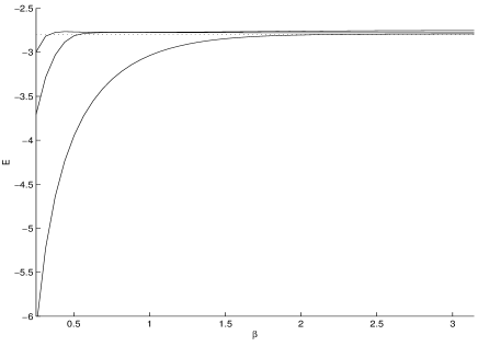
Figure 2: The dependence of several lower eigenvalues of $H_{2}(\alpha=0,\widetilde{Y})$ on the angle $\beta$. The dotted line is the threshold $E_{0}$.

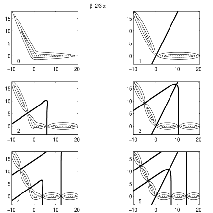
Figure 3: Eigenfunctions of six lower states of $H_{2}(\alpha=0,\widetilde{Y})$ for $\beta=2/3\pi$. Only the ground state has energy below the threshold $E_{0}$. The bold curves represent the nodal lines, the contours showing horizontal cuts correspond to a logarithmic scale.

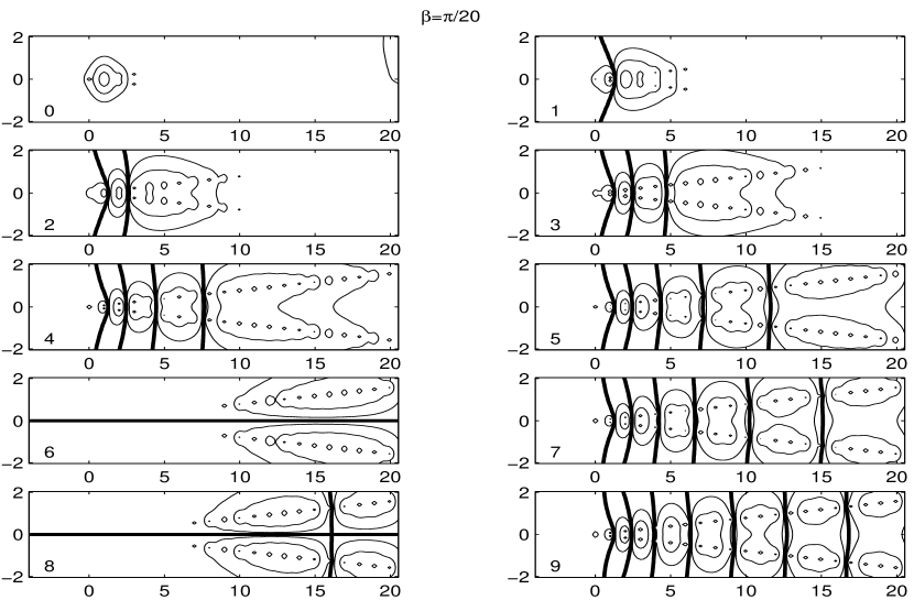
Figure 4: Eigenfunctions of ten lowest states of $H_{2}(\alpha=0,\widetilde{Y})$ for $\beta=\pi/20$. First five states correspond to eigenvalues of $H_{2}(0,\beta)$, the rest would belong to the essential spectrum in the limit $M\to\infty$. The bold curves represent the nodal lines, the contours showing horizontal cuts correspond to a logarithmic scale.

In the proof of Theorem 4.1 we observed that pairs of mutually close point interactions are crucial for the lower part of discrete spectrum if $\beta$ is small. This behaviour can be also demonstrated on the corresponding eigenfunctions, compare the contour graphs in Fig. 3 to those in Fig. 4. They represent several lowest states of $H_{2}(\alpha=0,\widetilde{Y})$ for the angles $\beta=2/3\pi$ and $\beta=\pi/20$, respectively. As indicated above, higher eigenfunction will correspond to the continuous spectrum in the limit $M\to\infty$. This applies to the eigenfunctions in Fig. 3, except the first one which approximates the ground state of $H_{2}(0,2/3\pi)$. In this case it is the only state which approximates an eigenstate of the infinite star. For a much smaller $\beta$ in Fig. 4 there are five eigenvalues below the threshold (number $0,1,2,3,4$ in the figure), which correspond to the discrete spectrum of $H_{2}(0,\pi/20)$. Notice that the remaining eigenfunctions resemble a standing-wave pattern along the graph arms as one would expect from an approximation from a generalized eigenfunction. It may seem that the graph number $5$ in Fig. 4 gives rise to a bound state too, but this only due to an insufficient length $M$ in our approximation.

5.3 A three-arm star

Here we consider $10$ point interactions on each arm and we put $l=1$ again. The behavior of eigenvalues is similar to the two-arm case, but the spectrum depends of two parameters $\beta_{1}$ and $\beta_{2}$. The minimum binding is achieved in the symmetric case as the graph of ground state energy of $H_{3}(\alpha=0,\widetilde{Y})$ in Fig. 5 shows. We see that the eigenvalue does not change much unless one of the angles becomes small. The ground state for the symmetric star, $\beta_{1}=\beta_{2}=2/3\pi$, is illustrated in Fig. 6; we see the logarithmic singularities at the point-interaction sites and the overall exponential decay of the eigenfuction along the graph arms.

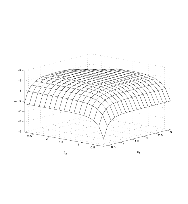
Figure 5: Ground state energy of $H_{3}(\alpha=0,\widetilde{Y})$.

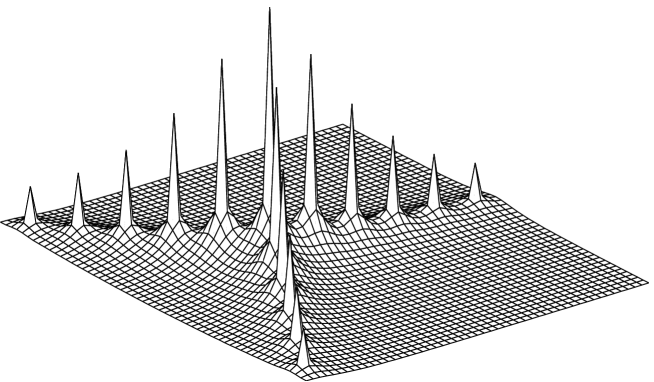
Figure 6: Ground state of $H_{3}(\alpha=0,\widetilde{Y})$ for $\beta_{1}=\beta_{2}=2/3\pi$ which approximates the ground state of $H_{3}(0,(2/3\pi,2/3\pi))$.

5.4 Larger $N$

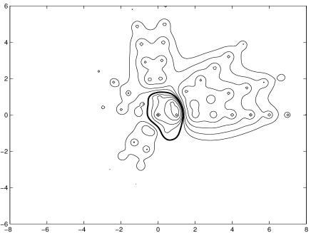
Figure 7: Eigenfunction of third excited state of $H_{10}(\alpha=0,\widetilde{Y})$ for $\beta=(0.3,0.7,1.5,1.8,2.5,3,4,4.4,5.2)$. It approximates an eigenfunction of $H_{10}(0,\beta)$. The bold curve represents the nodal line, the contours showing horizontal cuts correspond to a logarithmic scale.

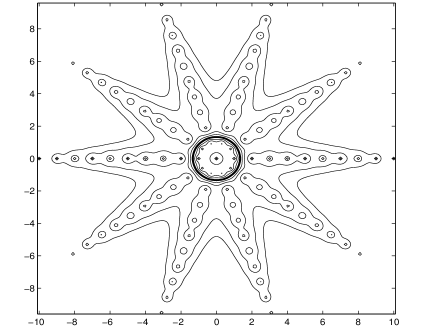
Figure 8: Eigenfunction of third excited state of $H_{10}(\alpha=0,\widetilde{Y})$ for $\beta=(\pi/5,2/5\pi,\ldots,9/5\pi)$. It approximates an eigenfunction of $H_{10}(0,\beta)$. The bold curve represents the nodal line, the contours showing horizontal cuts correspond to a logarithmic scale.

In a similar way one can treat star graphs with larger $N$. In order not to overload the paper with the illustrations, we restrict ourselves to a single example with $N=10$. The nodal line plots on the above pictures call to mind the question whether an eigengunction can have a closed nodal line. Such states can be found in spectrum of $H_{10}(\alpha,\widetilde{Y})$ for $\alpha=0$, as it is illustrated in Fig. 7 and Fig 8 for a non-symmetric and symmetric star. One of many mathematical questions which can be asked within the present model is about the minimum number $N$ for which this is possible.

Acknowledgment

The authors are grateful to V. Geyler and K. Pankrashkin for a useful discussion. The research was partially supported by GAAS under the contract #1048101.

References

• [AS] M.S. Abramowitz, I.A. Stegun, eds.: Handbook of Mathematical Functions, Dover, New York 1965.
• [AGHH] S. Albeverio, F. Gesztesy, R. Høegh-Krohn, H. Holden: Solvable Models in Quantum Mechanics, Springer, Heidelberg 1988.
• [BBK] G. Berkolaiko, E.B. Bogomolny, J.P. Keating: Star graphs and Šeba billiards, J. Phys. A34 (2001), 335-350.
• [BT] J.F. Brasche, A. Teta: Spectral analysis and scattering theory for Schrödinger operators with an interaction supported by a regular curve, in Ideas and Methods in Quantum and Statistical Physics, Cambridge Univ. Press 1992; pp. 197-211.
• [E1] P. Exner: Weakly coupled states on branching graphs, Lett. Math. Phys. 38 (1996), 313-320.
• [E2] P. Exner: Bound states of infinite curved polymer chains, Lett. Math. Phys., to appear; math-ph/0010046
• [EGŠT] P. Exner, R. Gawlista, P. Šeba, M. Tater: Point interactions in a strip, Ann. Phys. 252 (1996), 133-179.
• [EI] P. Exner, T. Ichinose: Geometrically induced spectrum in curved leaky wires, J. Phys. A34 (2001), 1439–1450.
• [EN] P. Exner, K. Němcová: Quantum mechanics of layers with a finite number of point perturbations, mp_arc 01–109; math–ph/0103030.
• [KS] V. Kostrykin, R. Schrader: Kirchhoff’s rule for quantum wires, J. Phys. A32 (1999), 595-630.
• [BMP] A.P. Prudnikov, Yu.O. Brychkov, O.I. Marichev: Integraly i rady, I. Elementarnye funkcii, II. Specialnye funkcii, Nauka, Moskva 1981–1983.
• [RS] K. Ruedenberg, C.W. Scherr: Free-electron network model for conjugated systems, I. Theory, J. Chem. Phys. 21 (1953), 1565-1581.
• [Ti] E.C. Titchmarch: Eigenfunction Expansions Associated with Second-Order Differential Equations, vol.II, Clarendon Press, Oxford 1958.
• [We] J. Weidmann: Linear Operators in Hilbert Space, Springer, N. Y. 1980.