New Developments in the Casimir Effect

Abstract

We provide a review of both new experimental and theoretical developments in the Casimir effect. The Casimir effect results from the alteration by the boundaries of the zero-point electromagnetic energy. Unique to the Casimir force is its strong dependence on shape, switching from attractive to repulsive as function of the size, geometry and topology of the boundary. Thus the Casimir force is a direct manifestation of the boundary dependence of quantum vacuum. We discuss in depth the general structure of the infinities in the field theory which are removed by a combination of zeta-functional regularization and heat kernel expansion. Different representations for the regularized vacuum energy are given. The Casimir energies and forces in a number of configurations of interest to applications are calculated. We stress the development of the Casimir force for real media including effects of nonzero temperature, finite conductivity of the boundary metal and surface roughness. Also the combined effect of these important factors is investigated in detail on the basis of condensed matter physics and quantum field theory at nonzero temperature. The experiments on measuring the Casimir force are also reviewed, starting first with the older measurements and finishing with a detailed presentation of modern precision experiments. The latter are accurately compared with the theoretical results for real media. At the end of the review we provide the most recent constraints on the corrections to Newtonian gravitational law and other hypothetical long-range interactions at submillimeter range obtained from the Casimir force measurements.

, ,

Contents
1	Introduction			1
	1.1	Zero-point oscillations and their manifestation		1.1
	1.2	The Casimir effect as a macroscopic quantum effect		1.2
	1.3	The role of the Casimir effect in different fields of physics		1.3
	1.4	What has been accomplished during the last years?		1.4
	1.5	The structure of the review		1.5
2	The Casimir effect in simple models			2
	2.1	Quantized scalar field on an interval		2.1
	2.2	Parallel conducting planes		2.2
	2.3	One- and two-dimensional spaces with nontrivial topologies		2.3
	2.4	Moving boundaries in a two-dimensional space-time		2.4
3	Regularization and renormalization of the vacuum energy			3
	3.1	Representation of the regularized vacuum energy		3.1
		3.1.1	Background depending on one Cartesian coordinate	3.1.1
		3.1.2	Spherically symmetric background	3.1.2
	3.2	The heat kernel expansion		3.2
	3.3	The divergent part of the ground state energy		3.3
	3.4	Renormalization and normalization conditions		3.4
	3.5	The photon propagator with boundary conditions		3.5
		3.5.1	Quantization in the presence of boundary conditions	3.5.1
		3.5.2	The photon propagator	3.5.2
		3.5.3	The photon propagator in plane parallel geometry	3.5.3
4	Casimir effect in various configurations			4
	4.1	Flat boundaries		4.1
		4.1.1	Two semispaces and stratified media	4.1.1
		4.1.2	Rectangular cavities: attractive or repulsive force?	4.1.2
	4.2	Spherical and cylindrical boundaries		4.2
		4.2.1	Boundary conditions on a sphere	4.2.1
		4.2.2	Analytical continuation of the regularized ground state energy	4.2.2

		4.2.3	Results on the Casimir effect on a sphere	4.2.3
		4.2.4	The Casimir effect for a cylinder	4.2.4
	4.3	Sphere (lens) above a disk: additive methods and proximity forces		4.3
	4.4	Dynamical Casimir effect		4.4
	4.5	Radiative corrections to the Casimir effect		4.5
	4.6	Spaces with non-Euclidean topology		4.6
		4.6.1	Cosmological models	4.6.1
		4.6.2	Vacuum interaction between cosmic strings	4.6.2
		4.6.3	Kaluza-Klein compactification of extra dimensions	4.6.3
5	Casimir effect for real media			5
	5.1	The Casimir effect at nonzero temperature		5.1
		5.1.1	Two semispaces	5.1.1
		5.1.2	A sphere (lens) above a disk	5.1.2
		5.1.3	The asymptotics of the Casimir force at high and low temperature	5.1.3
	5.2	Finite conductivity corrections		5.2
		5.2.1	Plasma model approach for two semispaces	5.2.1
		5.2.2	Plasma model approach for a sphere (lens) above a disk	5.2.2
		5.2.3	Computational results using the optical tabulated data	5.2.3
	5.3	Roughness corrections		5.3
		5.3.1	Expansion in powers of relative distortion amplitude:
			two semispaces	5.3.1
		5.3.2	Casimir force between nonparallel plates and plates covered
			by large scale roughness	5.3.2
		5.3.3	Casimir force between plates covered by short scale roughness	5.3.3
		5.3.4	Expansion in powers of relative distortion amplitude:
			a spherical lens above a plate	5.3.4
		5.3.5	Corrections to the Casimir force between a plate and a lens
			due to different kinds of roughness	5.3.5
		5.3.6	Stochastic roughness	5.3.6

	5.4	Combined effect of different corrections		5.4
		5.4.1	Roughness and conductivity	5.4.1
		5.4.2	Conductivity and temperature: two semispaces	5.4.2
		5.4.3	Conductivity and temperature: lens (sphere) above a disk	5.4.3
		5.4.4	Combined effect of roughness, conductivity and temperature	5.4.4
6	Measurements of the Casimir force			6
	6.1	General requirements for the Casimir force measurements		6.1
	6.2	Primary achievements of the older measurements		6.2
		6.2.1	Experiments with parallel plates by M.J. Sparnaay	6.2.1
		6.2.2	Experiments by Derjaguin et al.	6.2.2
		6.2.3	Experiments by D. Tabor, R. Winter and J. Israelachvili using
			mica cylinders	6.2.3
		6.2.4	Experiments of P. van Blokland and J. Overbeek	6.2.4
		6.2.5	Dynamical force mesurement techniques	6.2.5
	6.3	Experiment by S.K. Lamoreaux		6.3
	6.4	Experiments with the Atomic Force Microscope by Mohideen et al.		6.4
		6.4.1	First AFM experiment with aluminium surfaces	6.4.1
		6.4.2	Improved precision measurement with aluminium surfaces
			using the AFM	6.4.2
		6.4.3	Precision measurement with gold surfaces using the AFM	6.4.3
	6.5	Demonstration of the nontrivial boundary properties of
		the Casimir force		6.5
		6.5.1	Measurement of the Casimir force due to the corrugated plate	6.5.1
		6.5.2	Possible explanation of the nontrivial boundary dependence of
			the Casimir force	6.5.2
	6.6	The outlook for the measurements of the Casimir force		6.6

7	Constraints for non-Newtonian gravity from the Casimir effect		7
	7.1	Constraints from the experiments with dielectric test bodies	7.1
	7.2	Constraints from S.K. Lamoreaux experiment	7.2
	7.3	Constraints from the Casimir force measurements by means
		of atomic force microscope	7.3
8	Conclusions and discussion		8
Acknowledgements			Acknowledgements
Appendix A. Application of the Casimir force in nanotechnology			Appendix A. Applications of the Casimir force in nanotechnology
A1	Casimir force and nanomechanical devices		A.1
A2	Casimir force in nanoscale device fabrication		A.2
References			References

1 Introduction

More than 50 years have passed since H.B.G. Casimir published his famous paper [1] where he found a simple yet profound explanation for the retarded van der Waals interaction (which was described by him along with D. Polder [2] only a short time before) as a manifestation of the zero-point energy of a quantized field. For a long time, the paper remained relatively unknown. But starting from the 70ies this effect quickly received increasing attention and in the last few years has become highly popular. New high precision experiments on the demonstration of the Casimir force have been performed and more are under way. In theoretical developments considerable progress had been made in the investigation of the structure of divergencies in general, non-flat background and in the calculation of the effect for more complicated geometries and boundary conditions including those due to the real structures of the boundaries. In the Introduction we discuss the fundamental problems connected with the concept of physical vacuum, the role of the Casimir effect in different domains of physics and the scope of the review.

1.1 Zero-point oscillations and their manifestation

The Casimir effect in its simplest form is the interaction of a pair of neutral, parallel conducting planes due to the disturbance of the vacuum of the electromagnetic field. It is a pure quantum effect – there is no force between the plates (assumed to be neutral) in classical electrodynamics. In the ideal situation, at zero temperature for instance, there are no real photons in between the plates. So it is only the vacuum, i.e., the ground state of quantum electrodynamics (QED) which causes the plates to attract each other. It is remarkable that a macroscopic quantum effect appears in this way.

In fact the roots of this effect date back to the introduction by Planck in 1911 of the half quanta [3]. In the language of quantum mechanics one has to consider a harmonic oscillator with energy levels ${E}_{n}=\hbar{\omega}(n+\frac{1}{2})$, where $n=0,1,\dots$, and $\hbar$ is the Planck constant. It is the energy

$${E}_{0}={\hbar{\omega}\over 2}$$ (1.1)

of the ground state ($n=0$) which matters here. From the point of view of the canonical quantization procedure this is connected with the arbitrariness of the operator ordering in defining the Hamiltonian operator $\hat{H}$ by substituting in the classical Hamiltonian $H(p,q)$ the dynamical variables by the corresponding operators, $\hat{H}=H(\hat{p},\hat{q})$. It must be underlined that the ground state energy ${E}_{0}$ cannot be observed by measurements within the quantum system, i.e. in transitions between different quantum states, or for instance in scattering experiments. However, the frequency ${\omega}$ of the oscillator may depend on parameters external to the quantum system. It was as early as 1919 that this had been noticed in the explanation for the vapor pressure of certain isotopes, the different masses provide the necessary change in the external parameter (for a historical account see [4]).

In quantum field theory one is faced with the problem of ultraviolet divergencies which come into play when one tries to assign a ground state energy to each mode of the field. One has to consider then

$${E}_{0}={\hbar\over 2}\sum_{J}{\omega}_{J}\,,$$ (1.2)

where the index $J$ labels the quantum numbers of the field modes. For instance, for the electromagnetic field in Minkowski space the modes are labeled by a three vector ${\bf k}$ in addition to the two polarizations. The sum (1.2) is clearly infinite. It was Casimir who was the first to extract the finite force acting between the two parallel neutral plates

$$F(a)=-{\pi^{2}\over 240}\ {\hbar c\over a^{4}}S$$ (1.3)

from the infinite zero-point energy of the quantized electromagnetic field confined in between the plates. Here $a$ is the separation between the plates, $S>>a^{2}$ is their area and $c$ is the speed of light.

To do this Casimir had subtracted away from the infinite vacuum energy of Eq. (1.2) in the presence of plates, the infinite vacuum energy of quantized electromagnetic field in free Minkowski space. Both infinite quantities were regularized and after subtraction, the regularization was removed leaving the finite result.

Note that in standard textbooks on quantum field theory the dropping of the infinite vacuum energy of free Minkowski space is motivated by the fact that energy is generally defined up to an additive constant. Thus it is suggested that all physical energies be measured starting from the top of this infinite vacuum energy in free space. In this manner effectively the infinite energy of free space is set to zero. Mathematically it is achieved by the so called normal ordering procedure. This operation when applied to the operators for physical observables puts all creation operators to the left of annihilation operators as if they commute [5, 6, 7]. It would be incorrect, however, to apply the normal ordering procedure in this simplest form when there are external fields or boundary conditions, e.g., on the parallel metallic plates placed in vacuum. In that case there is an infinite set of different vacuum states and corresponding annihilation and creation operators for different separations between plates. These states turn into one another under adiabatic changes of separation. Thus, it is incorrect to pre-assign zero energy values to several states between which transitions are possible. Because of this, the finite difference between the infinite vacuum energy densities in the presence of plates and in free space is observable and gives rise to the Casimir force.

It is important to discuss briefly the relation of the Casimir effect to other effects of quantum field theory connected with the existence of zero-point oscillations. It is well known that there is an effect of vacuum polarization by external fields. The characteristic property of this effect is some nonzero vacuum energy depending on the field strength. Boundaries can be considered as a concentrated external field. In this case the vacuum energy in restricted quantization volumes is analogous to the vacuum polarization by an external field. We can then say that material boundaries polarize the vacuum of a quantized field, and the force acting on the boundary is a result of this polarization.

The other vacuum quantum effect is the creation of particles from vacuum by external fields. In this effect energy is transfered from the external field to the virtual particles (vacuum oscillations) transforming them into the real ones. There is no such effect in the case of static boundaries. However, if the boundary conditions depend on time there is particle creation, in addition to a force (this is the so called non-stationary or dynamic Casimir effect).

A related topic to be mentioned is quantum field theory with boundary conditions. The most common part of that is quantum field theory at finite temperature in the Matsubara formulation (we discuss this subject here only in application to the Casimir force). The effects to be considered in this context can be divided into pure vacuum effects like the Casimir effect and those where excitations of the quantum fields are present, i.e., real particles in addition to virtual ones. An example is an atom whose spontaneous emission is changed in a cavity. Another example is the so called apparatus correction to the electron g-factor. Here, the virtual photons responsible for the anomaly $a_{e}=(g-2)/2$ of the magnetic moment are affected by the boundaries. In this case by means of the electron a real particle is involved and the quantity to be considered is the expectation value of the energy in a one electron state. The same holds for cavity shifts of the hydrogen levels. This topic, together with a number of related ones, is called “cavity QED”. In the methods used, a photon propagator obeying boundary conditions, this is very closely related to the quantum field theoretic treatment of the Casimir effect. However, the difference is “merely” that expectation values are considered in the vacuum state in one case and in one (or more) particle states in the other.

1.2 The Casimir effect as a macroscopic quantum effect

The historical path taken by Casimir in his dealings with vacuum fluctuations is quite different from the approaches discussed in the previous subsection (see for example [8]). In investigating long-range van der Waals forces in colloids together with his collaborator D. Polder he took the retardation in the electromagnetic interaction of dipoles into account and arrived at the so called Casimir-Polder forces between polarizable molecules [2]. This was later extended by E.M. Lifshitz [9] to forces between dielectric macroscopic bodies usually characterized by a dielectric constant ${\epsilon}_{0}$

$$F(a)=-{\pi^{2}\over 240}{\hbar c\over a^{4}}{({\epsilon}_{0}-1)^{2}\over({\epsilon}_{0}+1)^{2}}\varphi({\epsilon}_{0})\ S\,,$$ (1.4)

where $\varphi({\epsilon}_{0})$ is a tabulated function. In this microscopic description, the ideal conductor is obtained in the limit ${\epsilon}_{0}\to\infty$, the same Casimir force (1.3) emerges just as in the zero-point energy approach. The point is that in the limit of ideal conductors only the surface layer of atoms thought of as a continuum interacts with the electromagnetic field. Clearly, in this idealized case, boundary conditions provide an equivalent description with the known consequences on the vacuum of the electromagnetic field. These alternative descriptions also work for deviations from the ideal conductor limit. For example, the vacuum interaction of two bodies with finite conductivity can be described approximately by impedance boundary conditions with finite penetration depth in one case and by the microscopic model on the other. For two dielectric bodies of arbitrary shape the summation of the Casimir-Polder interatomic potentials was shown to be approximately equal to the exact results if special normalizations accounting for the non-additivity effects are performed [10]. Only recently has an important theoretical advance occured in our understanding of this equivalence in the example of a spherical body (instead of two separate bodies). Here the equivalence of the Casimir-Polder summation and vacuum energy has been shown, at least in the dilute gas approximation [11].

The microscopic approach to the theory of both van der Waals and Casimir forces can be formulated in a unified way. It is well known that the van der Waals interaction appears between neutral atoms of condensed bodies separated by distances which are much larger than the atomic dimensions. It can be obtained non-relativistically in second order perturbation theory from the dipole–dipole interaction energy [12]. Because the expectation values of the dipole moment operators are zero, the van der Waals interaction is due to their dispersions, i.e. to quantum fluctuations. Thus, it is conventional to speak about fluctuating electromagnetic field both inside the condensed bodies and also in the gap of a small width between them. Using the terminology of Quantum Field Theory, for closely spaced macroscopic bodies the virtual photon emitted by an atom of one body reaches an atom of the second body during its lifetime. The correlated oscillations of the instantaneously induced dipole moments of those atoms give rise to the non-retarded van der Waals force [13, 14].

Let us now increase the distance between the two macroscopic bodies to be so large that the virtual photon emitted by an atom of one body cannot reach the second body during its lifetime. In this case the usual van der Waals force is absent. Nevertheless, the correlation of the quantized electromagnetic field in the vacuum state is not equal to zero at the two points where the atoms belonging to the different bodies are situated. Hence nonzero correlated oscillations of the induced atomic dipole moments arise once more, resulting in the Casimir force. In this theoretical approach the latter is also referred to as the retarded van der Waals force [7]. In the case of perfect metal the presence of the bounding condensed bodies can be reduced to boundary conditions at the sides of the gap. In the general case it is necessary to calculate the interaction energy in terms of the frequency dependent dielectric permittivity (and, generally, also the magnetic permeability) of the media. For the case of two semispaces with a gap between them this was first realised in [9] where the general expressions for both the van der Waals and Casimir force were obtained. Needless to say that this theoretical approach is applicable only for the electromagnetic Casimir effect caused by some material boundaries having atomic structure. The case of quantization volumes with non-trivial topology which also lead to the boundary conditions [15, 16, 17] is not covered by it.

An important feature of the Casimir effect is that even though it is quantum in nature, it predicts a force between macroscopic bodies. For two plane-parallel metallic plates of area $S=1\,{\rm cm}^{2}$ separated by a large distance (on the atomic scale) of $a=1\,\mu$m the value of the attractive force given by Eq. (1.3) is $F(a)\approx 1.3\times 10^{-7}\,$N. This force while small, is now within the range of modern laboratory force measurement techniques. Unique to the Casimir force is its strong dependence on shape, switching from attractive to repulsive as a function of the geometry and topology of a quantization manifold [18, 19]. This makes the Casimir effect a likely candidate for applications in nanotechnologies and nanoelectromechanical devices. The attraction between neutral metallic plates in a vacuum was first observed experimentally in [20]. This and other recent experimental developments in the measurement of the Casimir force is discussed in Sec.6.

There exist only a few other macroscopic manifestations of quantum phenomena. Among them there are the famous ones such as Superconductivity, Superfluidity, and the Quantum Hall Effect. In the above macroscopic quantum effects the coherent behaviour of large number of quantum particles plays an important role. In line with the foregoing the Casimir force arises due to coherent oscillations of the dipole moments of a great number of atoms belonging to the different boundary bodies. For this reason the Casimir effect can be considered also as a macroscopic quantum effect. The clearest implication of the above is that the greater attention traditionally given to the macroscopic quantum effects will also be eventually received by the Casimir effect.

1.3 The role of the Casimir effect in different fields of physics

The Casimir effect is an interdisciplinary subject. It plays an important role in a variety of fields of physics such as Quantum Field Theory, Condensed Matter Physics, Atomic and Molecular Physics, Gravitation and Cosmology, and in Mathematical Physics [21].

In Quantum Field Theory, the Casimir effect finds three main applications. In the bag model of hadrons in Quantum Chromodynamics the Casimir energy of quark and gluon fields makes essential contributions to the total nucleon energy. In Kaluza-Klein field theories Casimir effect offers one of the most effective mechanisms for spontaneous compactification of extra spatial dimensions. Moreover, measurements of the Casimir force provide opportunities to obtain more strong constraints for the parameters of long-range interactions and light elementary particles predicted by the unified gauge theories, supersymmetry, supergravity, and string theory.

In Condensed Matter Physics, the Casimir effect leads to attractive and repulsive forces between the closely spaced material boundaries which depend on the configuration geometry, on temperature, and on the electrical and mechanical properties of the boundary surface. It is responsible for some properties of thin films and should be taken into account in investigations of surface tension and latent heat. The Casimir effect plays an important role in both bulk and surface critical phenomena.

In Gravitation, Astrophysics and Cosmology, the Casimir effect arises in space-times with non-trivial topology. The vacuum polarization resulting from the Casimir effect can drive the inflation process. In the theory of structure formation of the Universe due to topological defects, the Casimir vacuum polarization near the cosmic strings may play an important role.

In Atomic Physics, the long-range Casimir interaction leads to corrections to the energy levels of Rydberg states. A number of the Casimir-type effects arise in cavity Quantum Electrodynamics when the radiative processes and associated energy shifts are modified by the presence of the cavity walls.

In Mathematical Physics, the investigation of the Casimir effect has stimulated the development of powerful regularization and renormalization techniques based on the use of zeta functions and heat kernel expansion.

The majority of these applications will be discussed below and the references to the most important papers will be also given.

1.4 What has been accomplished during the last years?

This review is devoted to new developments in the Casimir effect. In spite of the extensive studies on the subject performed in the more than 50 years there is only a small number of review publications. The first two large reviews [22, 23] were published more than ten years ago. There is a single monograph [24] specially devoted to the different aspects of the Casimir effect (the first, Russian, edition of it was published in 1990). The other monograph [25] is mostly concerned with the condensed matter aspects of the subject. Several chapters of the monograph [7] are also devoted to the Casimir effect.

There are at least three very important new developments in the Casimir effect which have made their appearance after the publication of the above mentioned reviews. The first falls within the domain of Quantum Field Theory. It has been known that in the case of flat boundaries the vacuum energy turns into infinity at large momenta in the same way as in free Minkowski space. Thus it is apparently enough to subtract the contribution of Minkowski space in order to obtain the final physical result for the Casimir energy. For arbitrary compact domains bounded by closed surfaces (for example, the interior of a sphere) this is, however, not the case. Except for the highest infinity (which is proportional to the fourth power of a cut-off momentum) there exist lower order infinities. The investigation of the general structure of these infinities for an arbitrary domain was a theoretical problem which had been solved by the combination of zeta-functional regularization [26, 27] and heat kernel expansion [28]. However, these results had been obtained mostly in the context of curved space-time. The explicit application to the Casimir effect was done later, first in [29, 30], where as an example the known divergencies for the Casimir effect for a massive field with boundary conditions on a sphere had been related to the corresponding heat kernel coefficients. In the nineties essential progress had been made in the understanding and application of zeta functions [31, 32] as well as in the calculation of the Casimir effect for massive fields for nonplane boundaries, e.g., in [33].

The second important development in the Casimir effect during the last years is concerned with Condensed Matter Physics. It has long been known that there are large corrections to the ideal field-theoretical expressions for the Casimir force due to several factors which are necessarily present in any experimental situation. The most important factors of this sort are those due to the finiteness of the conductivity of the boundary metal, surface roughness, and nonzero temperature. In the papers [34, 35, 36, 37, 38, 39] the Casimir force including these factors was investigated in detail. In doing so not only the influence of each individual factor was examined, but also their combined action was determined. This gave the possibility to increase the degree of agreement between theory and experiment.

Probably, the third development is the most striking. It consists in new, more precise measurements of the Casimir force between metallic surfaces. In [40] a torsion pendulum was used to measure the force between Cu plus Au coated quartz optical flat, and a spherical lens. In [41, 42, 43, 44] an atomic force microscope was first applied to measure the Casimir force between Al plus Au/Pd and Au coated sapphire disk and polystyrene sphere. Considerable progress has been made towards the improving the accuracy of the Casimir force measurements. The results of these measurements have allowed the stringent calculation of constraints on hypothetical forces such as ones predicted by supersymmetry, supergravity, and string theory [45, 46, 47, 48]. Other important results in the Casimir effect obtained during the last few years are also discussed below (see the review paper [49], and resource letter [50]).

1.5 The structure of the review

In the present review both the theoretical and experimental developments mentioned above are considered in detail. In Section 2 the simplified overview of the subject is provided. The main theoretical concepts used in the theory of the Casimir effect are illustrated here by simple examples, where no technical difficulties arise and all calculations can be performed in a closed form. Thus, the concepts of regularization and renormalization are demonstrated for the case of a scalar field on an interval and for the simplest spaces with nontrivial topology. The famous Casimir formula (1.3) for the force between perfectly conducting parallel plates is derived by two methods. The additional effects arising for moving boundaries are considered in two-dimensional space-time. The presentation is designed to be equally accessible to field theorists, specialists in condensed matter and experimentalists.

Section 3 contains the general field-theoretical analyses of regularization and renormalization procedures for the quantized field in an arbitrary quantization domain with boundaries. Here the divergent parts of the vacuum state energy and effective action are found by a combination of heat kernel expansion and zeta-functional regularization. Different representations for the regularized vacuum energy are obtained. The correspondence between the massive and massless cases is discussed in detail.

In Section 4 the Casimir energies and forces in a number of different configurations are calculated, among which are stratified media, rectangular cavities, wedge, sphere, cylinder, sphere (lens) above a disk and others. Different kinds of boundary conditions are considered and possible applications to the bag model of hadrons, Kaluza-Klein field theories, and cosmology are discussed. Radiative corrections to the Casimir effect are also presented. Both exact and approximate calculation methods are used in Sec.4. Some of the obtained results (especially the ones for the stratified media and a sphere above a disk) are of principal importance for the following sections devoted to aspects of condensed matter physics and of the experiments.

Section 5 is devoted to the consideration of the Casimir force for the real media. Here the Casimir force with account of nonzero temperature, finite conductivity of the boundary metal and surface roughness is investigated. The finite conductivity corrections are found both analytically in the framework of the plasma model of metals and numerically using the optical tabulated data for the complex refractive index. Surface roughness is taken into account by means of perturbation theory in powers of small parameter which is relates the effective roughness amplitude to the distance between the boundary surfaces. Special attention is paid to the combined effect of roughness and conductivity corrections, conductivity and temperature corrections, and also of all three factors acting together. It is shown that there are serious difficulties when applying the well known general expression for the temperature Casimir force [9] in the case of real metals. A line of attack on this problem is advanced.

In Section 6 the experiments on measuring the Casimir force are first reviewed. The presentation begins with the discussion of experimental problems connected with the measuring of small forces and small separations. Different background effects are also considered in detail. The historical experiments on measuring the Casimir force between metals and dielectrics are presented starting from [20]. The major part of Sec.6 is devoted to the presentation of the results of modern experiments [40, 41, 42, 43, 44] and their comparison with the theoretical results for the Casimir force between real media represented in Sec.5. The prospects for further improving the accuracy of Casimir force measurements are outlined.

In Section 7 the reader finds new interesting applications of the Casimir effect for obtaining constraints on the parameters of hypothetical long-range interactions including corrections to Newtonian gravitational law and light elementary particles predicted by the modern theories of fundamental interactions. Both the constraints following from the historical and modern experiments on measuring the Casimir force are presented. They are the best ones in comparison to all the other laboratory experiments in a wide interaction range. With further improvements in the Casimir force measurements the obtained constraints can further be strengthened.

The presentation is organized in such a way that the specialists in different fields of physics and also students could restrict their reading to some selected sections. For example, those who are interested in condensed matter aspects of the Casimir effect could read only the Secs.1, 2, 4.1.1, 4.3 and 5. Those who are also interested in experimental aspects of the problem may add to this Secs.6 and 7. Except for the purely theoretical Sec. 3 we are preserving in all formulas the fundamental constants $\hbar$ and $c$, as experimentalists usually do, which helps physical understanding.

2 The Casimir effect in simple models

In this section we present the elementary calculation of the Casimir energies and forces for several simple models. These models are mainly low-dimensional ones. Also the classical example of two perfectly conducting planes is considered. Such important concepts as regularization and renormalization are illustrated here in an intuitive manner readily accessible to all physicists, including non-specialists in Quantum Field Theory. Introduction into the dynamical Casimir effect is given at the end of the section.

2.1 Quantized scalar field on an interval

We start with a real scalar field $\varphi(t,x)$ defined on an interval $0<x<a$ and obeying boundary conditions

$$\varphi(t,0)=\varphi(t,a)=0\,.$$ (2.1)

This is the typical case where the Casimir effect arises. The simplicity of the situation (one dimensional space and one component field) gives the possibility to discuss the problems connected with the calculation of the Casimir force in the most transparent manner. In Sec. 2.2 a more realistic case of the quantized electromagnetic field between perfectly conducting planes will be considered.

The scalar field equation is as usual [5, 6]

$$\frac{1}{c^{2}}{\partial^{2}\varphi(t,x)\over\partial t^{2}}-{\partial^{2}\varphi(t,x)\over\partial x^{2}}+{m^{2}c^{2}\over\hbar^{2}}\varphi(t,x)=0\,,$$ (2.2)

where $m$ is the mass of the field. The indefinite scalar product associated with Eqs. (2.1), (2.2) is

$$(f,g)=i\int_{0}^{a}dx\left(f^{*}\partial_{x_{0}}g-\partial_{x_{0}}f^{*}g\right)\,,$$ (2.3)

where $f,g$ are two solutions of (2.2), $x_{0}\equiv ct$. We remind the reader that the scalar field in two-dimensional space-time is dimensionless. It is easy to check that the positive- and negative-frequency solutions of (2.2) obeying boundary conditions (2.1) are as follows

$$\varphi_{n}^{(\pm)}(t,x)=\left({c\over a{\omega}_{n}}\right)^{1/2}e^{\pm i{\omega}_{n}t}\sin k_{n}x\,,$$ (2.4)

$${\omega}_{n}=\left({m^{2}c^{4}\over\hbar^{2}}+c^{2}k_{n}^{2}\right)^{1/2}\,,\qquad k_{n}={\pi n\over a},\quad n=1,2,\dots\ .$$

They are orthonormalized in accordance with the scalar product (2.3)

$$\left(\varphi_{n}^{(\pm)},\varphi_{n^{\prime}}^{(\pm)}\right)=\mp\delta_{nn^{\prime}}\,,~{}~{}\left(\varphi_{n}^{(\pm)},\varphi_{n^{\prime}}^{(\mp)}\right)=0\,.\quad$$ (2.5)

We consider here a free field. Soliton-type solutions for the self-interacting field between the boundary points in two-dimensional space-time with different boundary conditions are considered in [51].

Now the standard quantization of the field is performed by means of the expansion

$$\varphi(t,x)=\sum_{n}\left[\varphi_{n}^{(-)}(t,x)a_{n}+\varphi_{n}^{(+)}(t,x)a_{n}^{+}\right]\,,$$ (2.6)

where the quantities $a_{n}$, $a_{n}^{+}$ are the annihilation and creation operators obeying the commutation relations

$$\left[a_{n},a_{n^{\prime}}^{+}\right]=\delta_{n,n^{\prime}},\quad\Big{[}a_{n},a_{n^{\prime}}\Big{]}=\left[a^{+}_{n},a_{n^{\prime}}^{+}\right]=0\,.$$ (2.7)

The vacuum state in the presence of boundary conditions is defined by

$$a_{n}\mid 0\rangle=0\,.$$ (2.8)

We are interested in investigating the energy of this state in comparison with the vacuum energy of the scalar field defined on an unbounded axis $-\infty<x<\infty$. The operator of the energy density is given by the $00$-component of the energy-momentum tensor of the scalar field in the two-dimensional space-time

$$T_{00}(x)={\hbar c\over 2}\left\{{1\over c^{2}}\left[\partial_{t}\varphi(x)\right]^{2}+\left[\partial_{x}\varphi(x)\right]^{2}\right\}\,.$$ (2.9)

Substituting Eq. (2.6) into Eq. (2.9) with account of (2.4), (2.7), and (2.8) one easily obtains

$$\langle 0\mid T_{00}(x)\mid 0\rangle={\hbar\over 2a}\sum_{n=1}^{\infty}{\omega}_{n}-{m^{2}c^{4}\over 2a\hbar}\sum_{n=1}^{\infty}{\cos 2k_{n}x\over{\omega}_{n}}\,.$$ (2.10)

The total vacuum energy of the interval $(0,a)$ is obtained by the integration of (2.10)

$${E}_{0}(a)=\int_{0}^{a}\langle 0\mid T_{00}(x)\mid 0\rangle dx=\frac{\hbar}{2}\sum_{n=1}^{\infty}{\omega}_{n}\,.$$ (2.11)

The second, oscillating term in the right-hand side of (2.10) does not contribute to the result.

The expression (2.11) for the vacuum state energy of the quantized field between boundaries is the standard starting point in the theory of the Casimir effect. Evidently the quantity ${E}_{0}(a)$ is infinite. It can be assigned a meaning by the use of some regularization procedure. There are many such regularization procedures discussed below. Here we use one of the simplest ones, i.e., we introduce an exponentially damping function $\exp(-\delta{\omega}_{n})$ after the summation sign. In the limit $\delta\to 0$ the regularization is removed. For simplicity let us consider the regularized vacuum energy of the interval for a massless field ($m=0$). In this case

$${E}_{0}(a,\delta)\equiv\frac{\hbar}{2}\sum_{n=1}^{\infty}{c\pi n\over a}\exp\left(-{\delta c\pi n\over a}\right)={\pi\hbar c\over 8a}\sinh^{-2}{\delta c\pi\over 2a}\,.$$ (2.12)

In the limit of small $\delta$ one obtains

$${E}_{0}(a,\delta)={\hbar a\over 2\pi c\delta^{2}}+{E}(a)+O(\delta^{2}),\ \ {E}(a)=-{\pi\hbar c\over 24a}\,,$$ (2.13)

i.e., the vacuum energy is represented as a sum of a singular term and a finite contribution.

Let us compare the result (2.13) with the corresponding result for the unbounded axis. Here instead of (2.4) we have the positive and negative frequency solutions in the form of traveling waves

$$\varphi_{k}^{(\pm)}(t,x)=\left({c\over 4\pi{\omega}}\right)^{1/2}e^{\pm i({\omega}t-kx)}\,,\ {\omega}=\left({m^{2}c^{4}\over\hbar^{2}}+c^{2}k^{2}\right)^{1/2},$$

$$\ -\infty<k<\infty\,.$$ (2.14)

The sum in the field operator (2.6) is interpreted now as an integral with the measure $dk/2\pi$, and the commutation relations contain delta functions $\delta(k-k^{\prime})$ instead of the Kronecker symbols. Let us call the vacuum state defined by

$$a_{k}\mid 0_{{\rm M}}\rangle=0$$ (2.15)

the Minkowski vacuum to underline the fact that it is defined in free space without any boundary conditions.

Repeating exactly the same simple calculation which was performed for the interval we obtain the divergent expression for the vacuum energy density in Minkowski vacuum

$$\langle 0_{M}\mid T_{00}(x)\mid 0_{M}\rangle={\hbar\over 2\pi}\int_{0}^{\infty}{\omega}dk\,,$$ (2.16)

and for the total vacuum energy on the axis

$${E}_{0M}(-\infty,\infty)={\hbar\over 2\pi}\int_{0}^{\infty}{\omega}dkL\,,$$ (2.17)

where $L\to\infty$ is the normalization length.

Let us separate the interval $(0,a)$ of the whole axis whose energy should be compared with (2.11)

$${E}_{0M}(a)={{E}_{0M}(-\infty,\infty)\over L}a={\hbar a\over 2\pi}\int_{0}^{\infty}{\omega}dk\,.$$ (2.18)

To calculate (2.18) we use the same regularization as above, i.e., we introduce the exponentially damping function under the integral. For simplicity consider once more the massless case

$${E}_{0M}(a)={c\hbar a\over 2\pi}\int_{0}^{\infty}ke^{-\delta ck}dk={\hbar a\over 2\pi c\delta^{2}}\,.$$ (2.19)

The obtained result coincides with the first term in the right-hand side of (2.13). Consequently, the renormalized vacuum energy of the interval $(0,a)$ in the presence of boundary conditions can be defined as

$${E^{\rm ren}_{0}}(a)\equiv\lim_{\delta\to 0}\left[{E}_{0}(a,\delta)-{E}_{0M}(a,\delta)\right]={E}(a)=-{\pi\hbar c\over 24a}\,.$$ (2.20)

It is quite clear that in this simplest case the renormalization corresponds to removing a quantity equal to the vacuum energy of the unbounded space in the given interval. The general structure of the divergencies of the vacuum energy will be considered in Sec. 3.3. The renormalized energy ${E}(a)$ monotonically decreases as the boundary points approach each other. This points to the presence of an attractive force between the conducting planes,

$$F(a)=-{\partial{E}(a)\over\partial a}=-{\pi\hbar c\over 24a^{2}\,.}$$ (2.21)

In the massive case $m\neq 0$ the above calculations lead to the result

$${E}(a,m)=-{mc^{2}\over 4}-{\hbar c\over 4\pi a}\int_{2\mu}^{\infty}{\sqrt{y^{2}-4\mu^{2}}\over\exp(y)-1}dy$$ (2.22)

with $\mu\equiv mca/\hbar$. Here the first, constant contribution is associated with the total energy of the wall (boundary point). It does not influence the force.

For $m=0$, Eq. (2.22) gives the same result as (2.20). It is possible to find the asymptotic behaviours of (2.22) in the case of small and large $\mu$. Thus, for $\mu<<1$ we have

$${E}(a,m)\approx-{mc^{2}\over 4}-{\pi\hbar c\over 24a}+{\hbar c\over 23\pi a}\mu^{2}\ln\mu\,,$$ (2.23)

and for $\mu>>1$

$${E}(a,m)\approx-{mc^{2}\over 2}-{\sqrt{\mu}\hbar c\over 4\sqrt{\pi}a}e^{-2\mu}\,.$$ (2.24)

Note, that the exponentially small value of the distance dependent term in the Casimir energy for $\mu>>1$ is typical. The same small value is also obtained for parallel planes in three-dimensional space and for fields of higher spin. It is, however, an artefact of plane boundaries. If some curvature is present, either in the boundary or in space-time, the behaviour is, generally speaking, in powers of the corresponding geometrical quantity, for example the radius of a sphere. There are only accidental exceptions to this rule, e.g., the case of a three sphere (see Sec. 4.6.2). Therefore it is primarily for plane boundaries and flat space that the Casimir effect for massless fields is larger and more important than that for massive fields.

Evidently, the physical results like those given by Eq. (2.20) or (2.22) should not depend on the chosen regularization procedure. We reserve the detailed discussion of this point for Sec. 3. It is not difficult, however, to make sure that the results (2.20), (2.22) actually do not depend on the specific form of the damping function. Let us, instead of the exponential function used above, use some function $f({\omega},\delta)$ with the following properties be given. The function $f({\omega},\delta)$ monotonically decreases with increasing ${\omega}$ or $\delta$ and satisfies the conditions $f({\omega},\delta)\leq 1$, $f({\omega},0)=1$, $f({\omega},\delta)\to 0$ for all $\delta\neq 0$ when ${\omega}\to\infty$.

The non-dependence of the obtained results on the form of $f({\omega},\delta)$ can be most easily demonstrated by the use of the Abel-Plana formula [52]

$$\sum\limits_{n=0}^{\infty}F(n)-\int\limits_{0}^{\infty}{\rm d}t~{}F(t)=\frac{1}{2}F(0)+i\int\limits_{0}^{\infty}{{\rm d}t\over e^{2\pi t}-1}\ {\left[F(it)-F(-it)\right]}\,,$$ (2.25)

where $F(z)$ is an analytic function in the right half-plane.

One can substitute $F(n)$ by ${\omega}_{n}$ multiplied by the damping function $f({\omega}_{n},\delta)$. Then the left-hand side of Eq. (2.25) can be interpreted as the difference in the regularized energies in the presence of boundaries and in free space from the Eq. (2.25) defining the renormalization procedure. The independence of the integral in the right-hand side of (2.25) on the form of $f({\omega}_{n},\delta)$ follows from the exponentially fast convergence which permits taking the limit $\delta\to 0$ under the integral (note that the Abel-Plana formula was first applied for the calculation of the Casimir force in [17]).

In the case of the Casimir effect for both scalar and spinor fields a modification of (2.25) is useful for the summation over the half-integer numbers

$$\sum\limits_{n=0}^{\infty}F(n+\frac{1}{2})-\int\limits_{0}^{\infty}{\rm d}t~{}F(t)=-i\int\limits_{0}^{\infty}{{\rm d}t\over e^{2\pi t}+1}\ {\left[F(it)-F(-it)\right]}\,.$$ (2.26)

Other generalizations of the Abel-Plana formula can be found in [24].

The Abel-Plana formulas are used in Secs. 2.2, 2.3, 4.1.2, and 4.6.1 to calculate the Casimir energies in different configurations.

2.2 Parallel conducting planes

As it was already mentioned in the Introduction, in its simplest case the Casimir effect is the reaction of the vacuum of the quantized electromagnetic field to changes in external conditions like conducting surfaces. The simplest case is that of two parallel perfectly conducting planes with a distance $a$ between them at zero temperature. They provide conducting boundary conditions to the electromagnetic field. These boundary conditions can be viewed as an idealization of the interaction of the metal surfaces with the electromagnetic field. In general, this interaction is much more complicated and is modified by the finite conductivity of the metal (or alternatively the skin depth of the electromagnetic field into the metal) and the surface roughness. But the idealized conducting boundary conditions are a good starting point for the understanding as they provide a complete problem and one that can be easily modified for the case of realistic metals. So it is possible to treat real metals with their finite conductivity and surface roughness as small perturbations (see Sec. 5). Here we focus on understanding the simple case of ideal metal boundaries.

It is well known in classical electrodynamics that both polarizations of the photon field have to satisfy boundary conditions

$${\mbox{${\bf{E}}_{t}$}}_{\bigl{|}_{S}}={\mbox{${\bf{H}}_{n}$}}_{\bigl{|}_{S}}=0$$ (2.27)

on the surface $S$ of perfect conductors. Here $\bf{n}$ is the outward normal to the surface. The index $t$ denotes the tangential component which is parallel to the surface $S$. The conditions (2.27) imply that the electromagnetic field can exist outside the ideal conductor only.

To proceed we imagine the electromagnetic field as a infinite set of harmonic oscillators with frequencies $\omega_{J}=c\sqrt{{\bf k}^{2}}$. Here the index of the photon momentum in free space (i.e., without boundaries) is $J={\bf k}=(k_{1},k_{2},k_{3})$ where all $k_{i}$ are continuous. In the presence of boundaries $J=(k_{1},k_{2},{\pi n\over a})=({\bf k}_{\perp},{\pi n\over a})$, where ${\bf k}_{\perp}$ is a two-dimensional vector, $n$ is integer. In the latter case the frequency results in

$$\omega_{J}={\omega}_{{\bf k_{\perp}},n}=c\sqrt{k_{1}^{2}+k_{2}^{2}+\left({\pi n\over a}\right)^{2}}\,.$$ (2.28)

This has to be inserted into the half sum over frequencies to get the vacuum energy of the electromagnetic field between the plates

$${E}_{0}(a)=\frac{\hbar}{2}\int{dk_{1}dk_{2}\over(2\pi)^{2}}\sum_{n=-\infty}^{\infty}\omega_{{\bf k_{\perp}},n}S\,,$$ (2.29)

where $S\to\infty$ is the area of plates. In contrast to Eq. (2.11) the sum is over negative integers also, so as to account for the two photon polarizations.

The expression obtained is ultraviolet divergent for large momenta. Therefore we have to introduce some regularization like discussed in the preceding section. This procedure is well known in quantum field theory and consists in changing the initial expression in a way that it becomes finite. This change depends on the so called regularization parameter and it is assumed that it can be removed formally by taking the limit value of this parameter to some appropriate value. Here, we perform the regularization by introducing a damping function of the frequency which was used in the original paper by Casimir (see also Sec. 2.1) and the modern zeta functional regularization. We obtain correspondingly

$${E}_{0}{(a,\delta)}=\frac{\hbar}{2}\int{dk_{1}dk_{2}\over(2\pi)^{2}}\sum_{n=-\infty}^{\infty}\omega_{{\bf k_{\perp}},n}e^{-\delta\omega_{{\bf k_{\perp}},n}}S$$ (2.30)

and

$${E}_{0}(a,s)=\frac{\hbar}{2}\sum_{n=-\infty}^{\infty}\int{dk_{1}dk_{2}\over(2\pi)^{2}}\ \omega_{{\bf k_{\perp}},n}^{1-2s}\ S\,.$$ (2.31)

These expressions are finite for $\delta>0$ respectively for ${\rm Re}s>\frac{3}{2}$ and the limits of removing the regularization are $\delta\to 0$ and $s\to 0$ correspondingly. The first regularization has an intuitive physical meaning. As any real body becomes transparent for high frequencies their contribution should be suppressed in some way which is provided by the exponential function. The regularization parameter $\delta$ can be viewed as somewhat proportional to the inverse plasma frequency. In contrast, the zeta-functional regularization does not provide such an explanation. Its advantage is more mathematical. The ground state energy in zeta-functional regularization ${E}_{0}(a,s)$ is the zeta function of an elliptic differential operator which is well known in spectral geometry. It is a meromorph function of $s$ with simple poles on the real axis for ${\rm Re}s\leq\frac{3}{2}$. To remove this regularization one has to construct the analytic continuation to $s=0$. In $s=0$ it may or may not have a pole (see examples below in Sec. 3). These properties give the zeta functional regularization quite important technical advantages and allow to simplify the calculations considerably. Together with this it must however be stressed that all regularizations must be equivalent as in the end they must deliver one and the same physical result.

Let us first consider the regularization done by introducing a damping function. The regularized vacuum energy of the electromagnetic field in free Minkowski space-time is given by

$${E}_{0M}(-\infty,\infty)={\hbar\over(2\pi)^{3}}\int d^{3}k{\omega}_{\bf k}e^{-\delta{\omega}_{\bf k}}LS\,,$$ (2.32)

where $L\to\infty$ is the length along the z-axis which is perpendicular to the plates, ${\omega}_{\bf k}=c|{\bf k}|=c\sqrt{k_{1}^{2}+k_{2}^{2}+k_{3}^{2}}$, ${\bf k}=(k_{1},k_{2},k_{3})$.

The renormalized vacuum energy is obtained by the subtraction from (2.30) of the Minkowski space contribution in the volume between the plates. After that the regularization can be removed. It is given by (compare (2.20))

$${E^{\rm ren}_{0}}(a) = \lim_{\delta\to 0}{\hbar\over 2}\int{dk_{1}dk_{2}\over(2\pi)^{2}}\left(\sum_{n=-\infty}^{\infty}{\omega}_{{\bf k}_{\perp},n}e^{-\delta{\omega}_{{\bf k}_{\perp},n}}-2a\int{{\rm d}k_{3}\over 2\pi}{\omega}_{\bf k}e^{-\delta{\omega}_{{\bf k}}}\right)S$$ (2.33)

$$= {c\hbar\pi\over a}\lim_{\delta\to 0}\int{dk_{1}dk_{2}\over(2\pi)^{2}}\left(\sum_{n=0}^{\infty}\sqrt{{k_{\perp}^{2}a^{2}\over\pi^{2}}+n^{2}}\ e^{\delta{\omega}_{{\bf k}_{\perp},n}}\right.$$

$$\left.-\int_{0}^{\infty}dt\sqrt{{k_{\perp}^{2}a^{2}\over\pi^{2}}+t^{2}}\ e^{-\delta{\omega}_{{\bf k}}}-{k_{\perp}a\over 2\pi}\right)S\,,$$

where $k_{\perp}^{2}\equiv k_{1}^{2}+k_{2}^{2}$, $t\equiv ak_{3}/\pi$.

To calculate (2.33) we apply the Abel-Plana formula (2.25) and obtain

$${E^{\rm ren}_{0}}(a)=-{c\hbar\pi^{2}\over a^{3}}\int_{0}^{\infty}ydy\int_{y}^{\infty}{\sqrt{t^{2}-y^{2}}\over e^{2\pi t}-1}dtS\,,$$ (2.34)

where $y=k_{\perp}a/\pi$ is the dimensionless radial coordinate in the $(k_{1},k_{2})$-plane. Note that we could put $\delta=0$ under the sign of the integrals in (2.34) due to their convergence. Also the signs when rounding the branch points $t_{1,2}=\pm iA$ of the function $F(t)=\sqrt{A^{2}+t^{2}}$ by means of

$$F(it)-F(-it)=2i\sqrt{t^{2}-A^{2}}~{}(t\geq A)$$ (2.35)

were taken into account.

To calculate (2.34) finally we change the order of integration and obtain

$${E^{\rm ren}_{0}}(a) = -{c\hbar\pi^{2}\over a^{3}}\int_{y}^{\infty}{dt\over e^{2\pi t}-1}\int_{0}^{t}y{\sqrt{t^{2}-y^{2}}}dyS$$ (2.36)

$$= -{c\hbar\pi^{2}\over 3a^{3}}{1\over(2\pi)^{4}}\int_{0}^{\infty}{dx\ x^{3}\over e^{x}-1}S=-{c\hbar\pi^{2}\over 720a^{3}}S\,.$$

The force (1.3) acting between the plates is obtained as derivative with respect to their distance

$$F(a)=-{\partial{E^{\rm ren}_{0}}(a)\over\partial a}=-{\pi^{2}\over 240}{\hbar c\over a^{4}}S\,.$$ (2.37)

Now we demonstrate the calculation of the ground state energy in zeta functional regularization starting from Eq. (2.31). Using polar coordinates $(k_{\perp},\varphi_{k})$ in the plane $(k_{1},k_{2})$ and performing the substitution $k_{\perp}=y{\pi n\over a}$ we obtain

$${E}_{0}(a,s)={\hbar c\over 2\pi}\int_{0}^{\infty}dy\ y\left(y^{2}+1\right)^{\frac{1}{2}-s}\sum_{n=1}^{\infty}\left({\pi n\over a}\right)^{3-2s}S\,.$$ (2.38)

Note that we put $s=0$ in the powers of some constants, e.g., $c$. The integration can be performed easily. The sum reduces to the well known Riemann zeta function ($t=2s-3$)

$$\zeta_{R}(t)=\sum_{n=1}^{\infty}{1\over n^{t}}\,,$$ (2.39)

which is defined for ${\rm Re}t>1$, i.e., ${\rm Re}s>\frac{3}{2}$, by this sum.

We need, however, the value of $\zeta_{R}(-3)$ in the limit of removing the regularization $s\to 0$. If we use the definition of $\zeta_{R}(t)$ according to the right-hand side of (2.39) this value evidently diverges. It is known that there exists a meromorph function with a simple pole in $t=-1$ ($s=1$) which can be obtained by analytic continuation of the right-hand side of Eq. (2.39) to the whole complex plane. Such analytic continuation is unique and well defined, for instance, at a point $t=-3$, although needless to say that its values for ${\rm Re}\ t\leq 1$ are not represented by the right-hand side of Eq. (2.39). It can be shown that the use of the value $\zeta_{R}(-3)=1/120$ instead of the infinite when $s\to 0$ value (2.38) is equivalent to the renormalization of the vacuum energy under consideration (the reasons for the validity of this statement are presented in Sec. 3). In this simplest case the value of the analytically continued zeta function can be obtained from the reflection relation

$$\Gamma\left(\frac{z}{2}\right)\pi^{-z/2}\zeta_{R}(z)=\Gamma\left({1-z\over 2}\right)\pi^{z-1\over 2}\zeta_{R}(1-z)\,,$$ (2.40)

where $\Gamma(z)$ is gamma function, taken at $z=4$. Substituting $\zeta_{R}(-3)=1/120$ into (2.38) and putting $s=0$ one obtains once more the renormalized physical energy of the vacuum (2.36) and attractive force acting between plates (2.37).

Here a remark must be added concerning the renormalization. The result which we obtained from the regularization by means of analytical continuation of zeta function into the complex $s$-plane is finite. This is particular to the case under consideration. In more complicated configurations the result will in general be infinite in the limit of removing the regularization so that some additional renormalization is needed. The situation for two plane plates considered above is referred to sometimes as renormalization by zeta functional regularization. It should be noted that it works in some special cases only.

2.3 One- and two-dimensional spaces with nontrivial topologies

As noted in the Introduction, when the space is topologically nontrivial the boundary conditions are imposed on the quantized field similar to the case of material boundaries. As a consequence, a nonzero vacuum energy appears, though there are no boundaries and therefore no force can act upon them. Let us return to the interval $0\leq x\leq a$ and impose boundary conditions

$$\varphi(t,0)=\varphi(t,a),\quad\partial_{x}\varphi(t,0)=\partial_{x}\varphi(t,a)\,,$$ (2.41)

which describe the identification of the boundary points $x=0$ and $x=a$. As a result we get the scalar field on a flat manifold with topology of a circle $S^{1}$ (see Fig. 1).

\begin{picture}(5.0,4.5)\put(0.0,0.0){\epsfbox{fig22.ps}} \end{picture}

Figure 1: Illustration of two flat manifolds with Euclidean topology (a) and topology of a circle (b).

Comparing with (2.1) now solutions are possible with $\varphi\neq 0$ at the points $x=0,a$. The orthonormal set of solutions to (2.2), (2.41) can be represented in the following form

$$\varphi^{(\pm)}_{n}(t,x)=\left(c\over 2a{\omega}_{n}\right)^{1/2}\exp\left[\pm i({\omega}_{n}t-k_{n}x)\right]\,,$$ (2.42)

$${\omega}_{n}=\left({m^{2}c^{4}\over\hbar^{2}}+c^{2}k_{n}^{2}\right)^{1/2}\,,\qquad k_{n}={2\pi n\over a},\quad n=0,\pm 1,\pm 2,\dots\ .$$

Substituting (2.42) into Eqs. (2.6) and (2.9) we obtain the vacuum energy density of a scalar field on $S^{1}$

$$\langle 0\mid T_{00}(x)\mid 0\rangle={\hbar\over 2a}\sum_{n=-\infty}^{\infty}{\omega}_{n}\,.$$ (2.43)

Here, as distinct from Eq. (2.10), no oscillating contribution is contained.

The total vacuum energy is

$${E}_{0}(a,m) = \int_{0}^{a}\langle 0\mid T_{00}(x)\mid 0\rangle\ dx={\hbar\over 2}\sum_{n=-\infty}^{\infty}{\omega}_{n}$$

$$= \hbar\sum_{n=0}^{\infty}{\omega}_{n}-{mc^{2}\over 2}\,.$$

The renormalization of this infinite quantity is performed by subtracting the contribution of the Minkowski space in accordance with (2.20). The simplest way to perform the calculation of the renormalized vacuum energy without introducing an explicit renomalization function is the use of the Abel-Plana formula (2.25). Substituting (2.42), (2.3) and (2.18) into (2.20) one obtains

$${E^{\rm ren}_{0}}(a,m) = \hbar\left[\sum_{n=0}^{\infty}{\omega}_{n}-{a\over 2\pi}\int_{0}^{\infty}{\omega}(k)dk\right]-{mc^{2}\over 2}$$

$$= {2\pi\hbar c\over a}\left[\sum_{n=0}^{\infty}\sqrt{A^{2}+n^{2}}-\int_{0}^{\infty}\sqrt{A^{2}+t^{2}}dt\right]-{mc^{2}\over 2}\,,$$

with $A\equiv amc/(2\pi\hbar)$ and the substitution $t=ak/(2\pi)$ was made.

Now we put $F(t)=\sqrt{A^{2}+t^{2}}$ into Eq. (2.25) and take account of Eq. (2.35). Substituting (2.25) into (2.3), we finally obtain

$${E^{\rm ren}_{0}}(a,m)=-{4\pi\hbar c\over a}\int_{A}^{\infty}{\sqrt{t^{2}-A^{2}\over e^{2\pi t}-1}}dt=-{\hbar c\over\pi a}\int_{\mu}^{\infty}{\sqrt{\xi^{2}-\mu^{2}}\over e^{\xi}-1}{\rm d}\xi\,,$$ (2.46)

where $\xi=2\pi t$, $\mu\equiv mca/\hbar=2\pi A$. Here the constant term describing the energy of a wall like in Eq. (2.22) is absent as there are no walls in space with non-Euclidean topology.

In the massless case we have $\mu=0$, and the result corresponding to (2.20) for the interval reads [19]

$${E^{\rm ren}_{0}}(a)=-{\hbar c\over\pi a}\int_{0}^{\infty}{\xi\over\exp(\xi)-1}d\xi=-{\pi\hbar c\over 6a}\,.$$ (2.47)

For $\mu>>1$ it follows from (2.46)

$${E^{\rm ren}_{0}}(a,m)\approx-{\sqrt{\mu}\hbar c\over\sqrt{2\pi}a}e^{-\mu}\,,$$ (2.48)

i.e., the vacuum energy of the massive field is exponentialy small which also happens in the case of flat spaces.

In the one-dimensional case $S^{1}$ is a single topologically nontrivial manifold. In two-dimensional spaces, i.e., (2+1)-dimensional space-times, there exist both flat and curved manifolds with non-Euclidean topology. Below we discuss one example of each.

A plane with the topology of a cylinder $S^{1}\times R^{1}$ is a flat manifold. This topology implies that points with Cartesian coordinates $(x+na,y)$, where $n=0,\pm 1,\pm 2,\dots$ are identified. For the scalar field $\varphi$ defined on that manifold the following boundary conditions hold

$$\varphi(t,0,y)=\varphi(t,a,y),\quad\partial_{x}\varphi(t,0,y)=\partial_{x}\varphi(t,a,y)\,.$$ (2.49)

Bearing in mind future applications to curved space-times for different dimensionality we remind the reader of the scalar wave equation in ($N+1$)-dimensional Riemannian space-time

$$\left(\nabla_{\kappa}\nabla^{\kappa}+\xi R+{m^{2}c^{2}\over\hbar^{2}}\right)\varphi(x)=0\,,$$ (2.50)

where $\nabla_{\kappa}$ is the covariant derivative, and $R$ is the scalar curvature of the space-time, $\xi=(N-1)/4N$, $x=(x_{0},x_{1},\dots,x_{N})$. This is the so called “equation with conformal coupling”. For zero mass it is invariant under conformal transformations (see [53, 54]). The equation with minimal coupling is obtained from (2.50) with $\xi=0$ for all $N$.

The metric energy-momentum tensor is obtained by varying the Lagrangian corresponding to (2.50) with respect to the metric tensor $g^{ik}$. Its diagonal components are [53, 54]

$$T_{ii} = \hbar c\left\{(1-2\xi)\partial_{i}\varphi\partial_{i}\varphi+(2\xi-\frac{1}{2})g_{ii}\partial_{k}\varphi\partial^{k}\varphi-\xi(\varphi\nabla_{i}\nabla_{i}\varphi+\nabla_{i}\nabla_{i}\varphi\ \varphi)\right.$$ (2.51)

$$\left.+\left[(\frac{1}{2}-2\xi){m^{2}c^{2}\over\hbar^{2}}g_{ii}-\xi G_{ii}-2\xi^{2}Rg_{ii}\right]\varphi^{2}\right\}\,,$$

where $G_{ik}=R_{ik}-\frac{1}{2}Rg_{ik}$ is the Einstein tensor, and $R_{ik}$ is the Ricci tensor.

Now let $N=2$, and the curvature be zero as in the case of $S^{1}\times R^{1}$. It is not difficult to find the orthonormalized solutions to Eq. (2.50) with the boundary conditions (2.49). All the preceding procedure described above for the case of $S^{1}$ can be repeated thereafter with the result [55]

$${E^{\rm ren}_{0}}(a,m)=-{\hbar c\over 4\pi a^{2}}\int_{\mu}^{\infty}{\xi^{2}-\mu^{2}\over\exp(\xi)-1}d\xi\ L\,,$$ (2.52)

where $L\to\infty$ is the normalization length along the $y$-axis as in Eq. (2.17). Note that this result is valid for an arbitrary value of $\xi$ and not for $\xi=\frac{1}{8}$ only.

In the massless case the integral in (2.52) is easily calculated with the result

$${E^{\rm ren}_{0}}(a)=-{\hbar c\zeta_{R}(3)\over 2\pi a^{2}}L\,,$$ (2.53)

where $\zeta_{R}(z)$ is the Riemann zeta function with $\zeta_{R}(3)\approx 1.202$. The calculation of the vacuum energy of the scalar field in other topologically non-trivial two-dimensional flat manifolds (a 2-torus, a Klein bottle, a Möbius strip of infinite width) can be found in [24].

We now consider the Casimir effect for a scalar field on a two-dimensional sphere $S^{2}$ with radius $a$. This is a curved manifold with scalar curvature $R=2a^{-2}$. In spherical coordinates the space-time metric reads

$$ds^{2}=c^{2}dt^{2}-a^{2}(d\theta^{2}+\sin^{2}\theta d\varphi^{2})\,.$$ (2.54)

The scalar field equation (2.50) with $\xi=\frac{1}{8}$, $R=2a^{-2}$ after the transformations takes the form

$${a^{2}\over c^{2}}\partial^{2}_{t}\varphi(x)-\Delta^{(2)}\varphi(x)+\left({m^{2}c^{2}a^{2}\over\hbar^{2}}+\frac{1}{4}\right)\varphi(x)=0\,,$$ (2.55)

where $\Delta^{(2)}$ is the angular part of the Laplace operator.

The orthonormal set of solutions to Eq. (2.50) obeying periodic boundary conditions in both $\theta$ and $\varphi$ can be represented as

$$\varphi^{(+)}_{lM}(t,\theta,\varphi)={\sqrt{c}\over a\sqrt{2{\omega}_{l}}}\exp(i{\omega}_{l}t)Y_{lM}(\theta,\varphi),\quad\varphi^{(-)}_{lM}(t,\theta,\varphi)=\left(\varphi^{(+)}_{lM}(t,\theta,\varphi)\right)^{*}\,,~{}~{}~{}$$

$${\omega}_{l}=\left[{m^{2}c^{4}\over\hbar^{2}}+{c^{2}\over a^{2}}(l+\frac{1}{2})^{2}\right]^{1/2},\quad l=0,1,2,\dots,~{}~{}M=0,\pm 1,\dots,\pm l,~{}~{}~{}$$ (2.56)

where $Y_{lM}(\theta,\varphi)$ are the spherical harmonics.

Substituting the field operator in the form (2.6) with eigenfunctions (2.3) into Eq. (2.51) we find the still non-renormalized vacuum energy density

$$\langle 0\mid T_{00}(x)\mid 0\rangle={\hbar\over 4\pi a^{2}}\sum_{l=0}^{\infty}\left(l+\frac{1}{2}\right){\omega}_{l}\,,$$ (2.57)

and the total vacuum energy of the sphere $S^{2}$ to be

$${E}_{0}(a,m)=\hbar\sum_{l=0}^{\infty}\left(l+\frac{1}{2}\right){\omega}_{l}\,.$$ (2.58)

The renormalization is performed according to (2.20), i.e., by introducing a regularization by means of a damping function and subtracting the contribution of the vacuum energy of the 3-dimensional Minkowski space-time. The final result which does not depend on the specific form of the damping function is most easily obtained by use of the Abel-Plana formula (2.26) for the summation over half-integers resulting in [56]

$${E^{\rm ren}_{0}}(a,m)=2mc^{2}\left({mca\over\hbar}\right)^{2}\int_{0}^{1}{\xi\sqrt{1-\xi^{2}}\over\exp(2\pi mca\xi/\hbar)+1}d\xi\,.$$ (2.59)

It is significant that here the Casimir energy is positive in contrast to the case of a flat manifold considered above.

When $\mu=mca/\hbar<<1$ it follows from (2.59) that

$${E^{\rm ren}_{0}}(a,m)\approx\frac{1}{3}mc^{2}\mu^{2}\,.$$ (2.60)

By this means, for a massless scalar field the Casimir energy on $S^{2}$ is equal to zero.

In the opposite limiting case $\mu>>1$ we have

$${E^{\rm ren}_{0}}(a,m)\approx{mc^{2}\over 24}\left[1-{7\over 40\mu^{2}}\right]\,.$$ (2.61)

As seen from (2.61) the Casimir energy on the surface of $S^{2}$ diminishes as a power of $\mu^{-1}$, whereas in the examples considered above it was exponentially small for $\mu>>1$. This is because the manifold $S^{2}$ has a nonzero curvature (see Sec. 3). For a sphere of infinite radius the total Casimir energy of a scalar field on $S^{2}$ takes the value ${E^{\rm ren}_{0}}(m)=mc^{2}/24$ (see the discussion of additional normalization condition for $m\to\infty$ in Sec.3.4).

2.4 Moving boundaries in a two-dimensional space-time

In the preceding sections we considered the case when the boundaries and boundary conditions are static. The corresponding vacuum energies and forces were also static. If the geometrical configuration, and, respectively, boundary conditions depend on time the so-called dynamic Casimir effect arises. The most evident manifestation of dynamic behavior is the dependence of the force on time. Let us return to a massless scalar field on an interval $(0,a)$ considered in Sec.2.1. Now let the right boundary depends on time: $a=a(t)$. It is obvious that in the first approximation the force also depends on time according to the same law as in (2.21)

$$F(a(t))=-{\pi\hbar c\over 24a^{2}(t)}\,.$$ (2.62)

This result is valid under the condition that the boundary velocity $a^{\prime}(t)$ is small compared with the velocity of light. The proof of this statement and the calculation of the velocity dependent corrections to the force can be found in Sec. 4.4 where more realistic dimensionalities are considered.

The other, and more interesting manifestation of the dynamic behavior is the creation of particles from vacuum by a moving boundary (this effect was first discussed in [57, 58]) The effect of creation of particles from vacuum by non-stationary electric and gravitational fields is well known (see, e.g., [53, 54]). As noted above, boundary conditions are idealizations of concentrated external fields. It is not surprising, then, that moving boundaries act in the same way as a non-stationary external field. We outline the main ideas of the effect of particle creation by moving boundaries with the same example of a massless scalar field defined on an interval $(0,a)$ with $a=a(t)$ depending on time when $t>0$.

Instead of (2.1) the boundary conditions now read

$$\varphi(t,0)=\varphi(t,a(t))=0\,.$$ (2.63)

For $t<0$ the orthonormalized set of solutions to Eq. (2.2) with $m=0$ is given by Eq. (2.4) in which one should substitute $a$ by $a_{0}\equiv a(0)$. The field operator which is understood now as in-field (i.e., field defined for $t<0$ when the boundary point is at rest) is given by the Eq. (2.6). For any moment the set of solutions to Eq. (2.2), $\chi_{n}^{(\pm)}(t,x)$ should satisfy the boundary conditions (2.63) and the initial condition

$$\chi_{n}^{(\pm)}(t\leq 0,x)=\varphi^{(\pm)}_{n}(t,x)=\frac{1}{\sqrt{\pi n}}e^{\pm i{\omega}_{n}t}\sin{\pi nx\over a_{0}}\,.$$ (2.64)

The field operator at any moment is given by

$$\varphi(t,x)=\sum_{n}\left[\chi^{(-)}_{n}(t,x)a_{n}+\chi^{(+)}_{n}(t,x)a_{n}^{+}\right]\,.$$ (2.65)

The functions $\chi_{n}^{(\pm)}(t,x)$ which are unknown for $t>0$ can be found in the form of a series (see, e.g., [59, 60])

$$\chi^{(-)}_{n}(t,x)=\frac{1}{\sqrt{\pi n}}\sum_{k}Q_{nk}(t)\sqrt{{a_{0}\over a(t)}}\sin{\pi kx\over a(t)}$$ (2.66)

with the initial conditions

$$Q_{nk}(0)=\delta_{nk},~{}~{}Q^{\prime}_{nk}(0)=-i{\omega}_{n}\delta_{nk}\,.$$ (2.67)

Here $Q_{nk}(t)$ are the coefficients to be determined, $n,k=1,2,3,\dots$. The positive-frequency functions $\chi^{(+)}_{n}$ are obtained as the complex conjugate of (2.66).

It is obvious that both boundary conditions (2.63) and the initial conditions (2.64) are satisfied automatically in (2.66). Substituting Eq. (2.66) into the field equation (2.2) (with $m=0$) we arrive after conversion to an infinite coupled system of differential equations with respect to the functions $Q_{nk}(t)$[60]

$$Q_{nk}^{\prime\prime}(t)+{\omega}_{k}^{2}(t)Q_{nk}(t)$$

$$=\sum_{j}\left[2\nu(t)h_{kj}Q_{nj}^{\prime}(t)+\nu^{\prime}(t)h_{kj}Q_{nj}(t)+\nu^{2}(t)\sum_{l}h_{jk}h_{jl}Q_{nl}(t)\right]\,.$$ (2.68)

Here the following notations are introduced

$${\omega}_{k}(t) = {c\pi k\over a(t)},~{}~{}~{}~{}\nu(t)={a^{\prime}(t)\over a(t)}\,,$$

$$h_{kj} = -h_{jk}=(-1)^{k-j}{2kj\over j^{2}-k^{2}},~{}~{}j\neq k\,.$$ (2.69)

Let after some time $T$ the right boundary of the interval return to its initial position $a_{0}$. For $t>T$ the right-hand side of Eq. (2.4) is equal to zero and the solution with initial conditions (2.67) can be represented as a linear combination of exponents with different frequency signs

$$Q_{nk}(t)=\alpha_{nk}e^{-i{\omega}_{k}t}+\beta_{nk}e^{i{\omega}_{k}t}\,.$$ (2.70)

This is a familiar situation which is well-known in the theory of particle creation from vacuum by a non-stationary external field. Substituting Eqs. (2.66) and (2.70) into the field operator (2.65) we represent it once more as the expansion in terms of the functions $\varphi^{(\pm)}_{k}$ from (2.4) where $m=0$, $a=a_{0}$ but with the new creation and annihilation operators

$$b_{k}=\sum_{n}\left(\sqrt{k\over n}\alpha_{nk}a_{n}+\sqrt{k\over n}\beta^{*}_{nk}a_{n}^{+}\right)$$ (2.71)

and the Hermitian conjugate for $b^{+}_{k}$.

Eq. (2.71) is the Bogoliubov transformation connecting in- creation and annihilation operators $a_{n}^{+},a_{n}$ with the out-ones $b^{+}_{n},b_{n}$. Its coefficients satisfy the equality

$$\sum_{k}k\left(|{\alpha}_{nk}|^{2}-|\beta_{nk}|^{2}\right)=n\,,$$ (2.72)

which is the unitarity condition (see [53, 54] for details).

Different vacuum states are defined for $T<0$ and for $t>T$ due to non-stationarity of the boundary conditions

$$a_{k}|0_{\rm in}>=0~{}\mbox{for}~{}t<0;~{}~{}~{}~{}~{}b_{k}|0_{\rm out}>=0~{}\mbox{for}~{}t>T\,.$$ (2.73)

The number of particles created in the $k$th mode is equal to the vacuum-vacuum matrix element in the in-vacuum of the out-operator for the number of particles. It is calculated with the help of Eqs. (2.71) and (2.73)

$$n_{k}=<0_{\rm in}|b^{+}_{k}b_{k}|0_{\rm in}>=k\sum_{n=1}^{\infty}\frac{1}{n}|\beta_{nk}|^{2}\,.$$ (2.74)

The total number of particles created by the moving boundary during time $T$ is

$$N=\sum_{k=1}^{\infty}n_{k}=\sum_{k=1}^{\infty}k\sum_{n=1}^{\infty}\frac{1}{n}|\beta_{nk}|^{2}\,.$$ (2.75)

It should be mentioned that in the original papers [57, 58] another method was used to calculate the number of created particles. There property that in two dimensional space-time the classical problem with non-stationary boundary conditions can be reduced to a static one by means of conformal transformations was exploited. This method, however, does not work in four-dimensional space-time.

To calculate the quantities (2.74) and (2.75) it is necessary to solve the system (2.4) which is a rather complicated problem. It is possible, however, to obtain a much more simple system in the case when the boundary undergoes small harmonic oscillations under the condition of a parametric resonance. Let us consider, following [61], the motion of the boundary according to the law

$$a(t)=a_{0}\left[1+{\epsilon}\sin(2{\omega}_{1}t)\right]\,,$$ (2.76)

where ${\omega}_{1}=c\pi/a_{0}$, and the non-dimensional amplitude of the oscillations is ${\epsilon}<<1$ (in realistic situations ${\epsilon}\sim 10^{-7}$). In the framework of the theory of the parametrically excited systems [62] the coefficients ${\alpha}_{nm}$, $\beta_{nm}$ can be considered as slowly varying functions of time. Substituting (2.70) into (2.4) we neglect by all the terms of the order ${\epsilon}^{2}$ and perform the averaging over fast oscillations with the frequencies of the order ${\omega}_{k}$. As a result the simplified system (2.4) takes the form [61]

$$\begin{array}[]{rclrcl}{d{\alpha}_{n1}\over d\tau}&=&-\beta_{n1}+3{\alpha}_{n3},&{d{\alpha}_{nk}\over d\tau}&=&(k+2){\alpha}_{n,k+2}-(k-2){\alpha}_{n,k-2},~{}k\geq 2\,,\\ {d\beta_{n1}\over d\tau}&=&-{\alpha}_{n1}+3\beta_{n3},&{d\beta_{nk}\over d\tau}&=&(k+2)\beta_{n,k+2}-(k-2)\beta_{n,k-2},~{}k\geq 2\,,\end{array}$$ (2.77)

where the initial conditions are

$${\alpha}_{nk}(0)=\delta_{nk},~{}~{}~{}\beta_{nk}(0)=0\,.$$ (2.78)

Here we introduce the so-called “slow time”

$$\tau=\frac{1}{2}{\epsilon}{\omega}_{1}t\,.$$ (2.79)

Note that even modes are not coupled to the odd modes in (2.77). Due to the initial conditions (2.78)

$$\beta_{n,2k}(t)=\beta_{2l,k}(t)=0\,,$$ (2.80)

which is to say that the particles are created in odd modes only.

The solution of the differential system (2.77) and (2.78) and of the integral equation which is equivalent to it can be found in [61]. Here we present only the final result for the particle creation rate. With the proviso that $\tau<<1$ the number of created particles and the creation rate in the lowest mode with $k=1$ are [61]

$$n_{1}(t)\approx\frac{1}{4}({\epsilon}{\omega}_{1}t)^{2},~{}~{}{dn_{1}(t)\over dt}\approx\frac{1}{2}{\epsilon}^{2}{\omega}_{1}^{2}t\,.$$ (2.81)

In the opposite limiting case $\tau>>1$ the results are

$$n_{1}(t)\approx\frac{4}{\pi^{2}}({\epsilon}{\omega}_{1}t)+\frac{2}{\pi^{2}}\ln 4-\frac{1}{2},~{}~{}{dn_{1}(t)\over dt}\approx\frac{4}{\pi^{2}}{\epsilon}{\omega}_{1}\,.$$ (2.82)

The total number of created particles in all modes is $N(t)\approx n_{1}(t)$ if $\tau<<1$, i.e., the lowest mode alone determines the result. However, if $\tau>>1$ we have $N(t)\sim\tau^{2}>>n_{1}(t)$.

For the energy of the particles created in the lowest mode one obtains evidently the result ${\omega}_{1}n_{1}(t)$. The total energy of particles created in all modes is

$$E(t)={\omega}_{1}\sum_{k}kn_{k}(t)=\frac{1}{4}{\omega}_{1}\sinh^{2}(2\tau)\,.$$ (2.83)

As is seen from this result the total energy increases faster than the total number of photons, i.e., the pumping of energy takes place into the high-frequency modes at the expense of the low-frequency ones.

In Sec. 4.4 where the three dimensional configurations will be considered we discuss the possibility of experimental observation of the photons created by the moving mirrors. Additional factors such as imperfectness of the boundary mirrors, back reaction of the radiated photons upon the mirror etc. will be discussed. The influence of the detector placed into the cavity will be also touched upon.

3 Regularization and renormalization of the vacuum energy

This section is devoted to the theoretical foundation of the Casimir effect. It contains the general regularization and renormalization procedures formulated in the frames of Quantum Field Theory under the influence of boundary conditions. The divergent part of the vacuum state energy is found in an arbitrary quantization domain. Different representations for the regularized vacuum energy are obtained. The photon propagator in the presence of boundary conditions is presented. The mathematical methods set forth in this section give the possibility to calculate the Casimir energies and forces for variety of configurations and quantized fields of different spin. Remind that in this section the units are used in which $\hbar=c=1$.

3.1 Representation of the regularized vacuum energy

The basic quantities appearing in quantum field theory in connection with the Casimir effect are the vacuum expectation value of the energy operator in the ground state (vacuum) of the quantum field under consideration and the corresponding effective action. In zeta functional regularization the ground state energy can be written as half sum over the one-particle energies $\epsilon_{J}$ labeled by some general index $J$

$${E}_{0}(s)=\pm\frac{1}{2}\mu^{2s}\sum_{J}{\epsilon_{J}}^{1-2s}\,.$$ (3.1)

The one-particle energies $\epsilon_{J}$ are by means of $\epsilon_{J}^{2}=\Lambda_{J}$ connected with the eigenvalues of the corresponding one particle Hamiltonian

$$H\Phi_{J}({\bf x})=\Lambda_{J}\Phi_{J}({\bf x})\,.$$ (3.2)

In case of a first order (in the derivatives) theory, e.g., for a spinor field, they have to be taken with positive sign, $\epsilon_{j}\to|\epsilon_{j}|$. We assume the spectrum to be discrete for the moment. Within the given regularization we are free to introduce an arbitrary constant $\mu$ with the dimension of a mass which assures the energy ${E}_{0}(s)$ to have the correct dimension. The different signs in Eq. (3.1) correspond to bosonic and fermionic fields respectively.

The mathematical background of the regularization used in (3.1) is the zeta function

$$\zeta_{H}(s)=\sum_{J}{\Lambda_{J}}^{-s}$$ (3.3)

associated with the operator $H$. Then the ground state energy (3.1) reads

$${E}_{0}(s)=\pm{\mu^{2s}\over 2}\zeta_{H}(s-\frac{1}{2})\,.$$ (3.4)

This zeta function is one of the functions defined on an operators spectrum and is used in field theory as well as in geometry. It is a well investigated object with a clearly defined meaning, especially for hyperbolic pseudo-differential operators. It is known to be a meromorphic function of $s$ and it has simple (sometimes double [63]) poles. This function coincides for ${\rm Re}s>d/p$ (where $d$ is the dimension of the manifold and $p$ the order of the differential operator, we consider operators with $p=2$ only) with the sum in the right-hand side of Eq. (3.3).

In a broader context, in quantum field theory instead of the ground state energy one considers the effective action $\Gamma$ which is defined by means of

$$\Gamma=-i\ln Z\,,$$ (3.5)

where $Z$ is the vacuum-to-vacuum transition amplitude. It can be represented by the functional integral

$$Z=\int D\Phi\ e^{iS(\Phi)}$$ (3.6)

taken over fields satisfying corresponding boundary conditions. In the context of ground state energy one usually restricts oneself to an action quadratic in the fields, i.e., to a free theory. A typical action reads

$$S(\Phi)=-\frac{1}{2}\int dx\ \Phi(x)(\Box+V(x)+m^{2})\Phi(x)\,,$$ (3.7)

where $V(x)$ is a background potential. So the integral (3.6) is Gaussian and can be carried out delivering

$$Z=(\det(\Box+V(x)+m^{2}))^{-\frac{1}{2}}=e^{-\frac{1}{2}{\rm Tr}\ln(\Box+V(x)+m^{2})}\,.$$ (3.8)

The box operator may be the usual wave operator or may be more complicated, for example $\Box\to D_{\mu}D^{\mu}$ with the covariant derivative $D_{\mu}=\partial_{\mu}+ieA_{\mu}(x)$ in case of the complex Klein-Gordon field in the background of an electromagnetic potential. The functional integral can also be over Grassmann fields too describing quantized fermion fields. In that case we have the usual changes in the sign so that the effective action may be written as

$$\Gamma=\pm\frac{i}{2}{\rm Tr}\ln(\Box+V(x)+m^{2})\,.$$ (3.9)

We need to give this expression a more precise meaning. Again, we assume the spectrum of the one particle Hamiltonian (3.2) to be discrete. Moreover, we assume the background to be static. In that case we can immediately switch to the Euclidean formulation and separate the time dependence by means of a Fourier transform to a momentum $p_{0}$. Then the effective action (3.9) becomes diagonal. Finally, we introduce the zeta functional regularization and the effective action can be written as

$$\Gamma=\mp{\partial\over\partial s}\mu^{2s}\int_{-\infty}^{\infty}{{\rm d}p_{0}\over 2\pi}\sum_{J}\left(p_{0}^{2}+\Lambda_{J}\right)^{-s}\,,~{}~{}(s\to 0)\,.$$ (3.10)

The integral over $p_{0}$ may be carried out and by means of Eq. (3.3) the effective action can be expressed in terms of the zeta function of the operator $H$

$$\Gamma=\mp{\partial\over\partial s}{\mu^{2s}\over\sqrt{4\pi}}{\Gamma(s-\frac{1}{2})\over\Gamma(s)}\ \zeta_{H}(s-\frac{1}{2})\,.$$ (3.11)

In this way, a connection between the ground state energy and the effective potential is established. In general, the physical consequences resulting from both quantities are expected to be the same. This will be seen after the discussion of the renormalization and the corresponding normalization conditions.

The quantities introduced so far have a precise mathematical meaning. However, they have a restricted region of applicability which is due to the assumption of a discrete spectrum which is here equivalent to a finite quantization volume. In order to go beyond that we are faced with the infinite Minkowski space contribution in problems with a flat background manifold. A typical example is the Casimir effect for the exterior of a ball. More precisely, let $L$ be the size of the quantization volume. Then the ground state energy (and the zeta function as well) for $L\to\infty$ contains a contribution which does not depend on the background and, by means of translational invariance, it will be proportional to the infinite volume of the Minkowski space. This contribution is independent of the background and thus of the boundary conditions. Because of this, it does not carry any information of interest. In the following we drop it without changing the notation of the corresponding quantities like ${E}_{0}$. Next, there is a contribution which does not depend on $L$ but depends on the background and which we are interested in. Finally there are contributions vanishing for $L\to\infty$.

To put this procedure into a mathematical framework it is useful to transform the sum, say in Eq. (3.1), into an integral. A second reason for this is the need to construct the analytic continuation of the zeta function to the left of ${\rm Re}s>s_{0}$ which is necessary for removing the regularization. There is no general procedure to do this and we are left with some special assumptions which are, however, still quite general and allow consideration of a wide class of problems. So we assume that the variables separate in the problems considered. The simplest example in this recpect is a background depending on one Cartesian coordinate only, e.g. parallel mirrors. The next example is a spherically symmetric background, say boundary conditions on a sphere or a potential $V(r)$. As known, separation of variables is connected with some symmetry. So the same can be done for a problem with cylindrical symmetry, for a generalized cone, for monopoles and quite a large number of other problems not considered here. We restrict ourselfs to the two most simple, but typical cases.

3.1.1 Background depending on one Cartesian coordinate

Here we assume the potential to depend on the coordinate $x_{3}$ only. In that case, by means of translational invariance, the vacuum energy is proportional to the volume of the directions $x_{\perp}$ perpendicular to $x_{3}$ and we have in fact to consider the corresponding energy density. With the obvious ansatz $\Phi_{J}({\bf x})=\exp(i{\bf k_{\perp}x_{\perp}})\Phi_{n}(x_{3})$ the equation for the one particle energy becomes one dimensional

$$H\Phi_{n}(x_{3})=\Lambda_{n}\Phi_{n}(x_{3})$$ (3.12)

with the operator

$$H=k_{\perp}^{2}-{d^{2}\over dx_{3}^{2}}+V(x_{3})+m^{2}\,.$$ (3.13)

It is meaningful to define the pure Schrödinger operator

$${\bf P}=-{d^{2}\over dx^{2}}+V(x)$$ (3.14)

with the eigenvalue problem which looks like a one dimensional Schrödinger equation

$${\bf P}\varphi_{n}(x)=\lambda_{n}\varphi_{n}(x)$$ (3.15)

so that Eq. (3.1) for the vacuum energy takes the form

$${E}_{0}(s)=\pm\frac{\mu^{2s}}{2}\sum_{n}\int{dk_{1}dk_{2}\over(2\pi)^{2}}\left(\lambda_{n}+k_{\perp}^{2}+m^{2}\right)^{1/2-s}\,.$$ (3.16)

Here we assume that the potential $V(x)$ for $x\to\pm\infty$ tends to zero (see Fig. 2). Otherwise, if it tends to a nonzero constant this constant can be absorbed into a redefinition of the mass $m$. The case when it tends to different constants at both infinities can be treated in a similar way and is not considered here.

Formula (3.16) can be rewritten by integrating out $k_{1}$ and $k_{2}$. By means of the substitution $k_{1,2}\to\sqrt{\lambda_{n}+m^{2}}k_{1,2}$ the expression factorizes. The $k$-integration reads simply

$$\int{dk_{1}dk_{2}\over(2\pi)^{2}}\left(k_{\perp}^{2}+1\right)^{1/2-s}={1\over 4\pi}\ {1\over s-3/2}\,.$$

The integral is defined for ${\rm Re}s>3/2$. The analytic continuation to the whole $s$-plane is given by the right-hand side. In more general cases, for instance when the number of dimensions of the directions perpendicular to $x_{3}$ is odd, a combination of gamma functions results. After this transformation the ground state energy takes the form

$${E}_{0}(s)=\pm{\mu^{2s}\over 8\pi}{1\over s-3/2}\sum_{n}\left(\lambda_{n}+m^{2}\right)^{3/2-s}\,.$$ (3.17)

Now, with the discrete eigenvalues ${\lambda}_{n}$, Eq. (3.17) is a well defined expression and we could start to construct its analytic continuation to $s=0$. An example for such a problem is the Casimir effect between two planes with Dirichlet boundary conditions at $x=\pm L$ and no potential, i.e., with $V(x)=0$ in Eq. (3.14), which was considered in Sec. 2.2. There, the remaining sum delivered the Riemann zeta function with its well known analytic continuation. But this is not the general case and in order to separate the translational invariant part (in $x_{3}$-direction) we proceed as follows.

We consider the one dimensional scattering problem on the whole axis ($x\in(-\infty,\infty)$) associated with the operator ${\bf P}$ (3.15)

$${\bf P}\varphi(x)=k^{2}\varphi(x)\,.$$ (3.18)

It is well investigated, please refer to the textbook [64] for example. We note the following properties. Eq. (3.18) has two linear independent solutions which can be chosen as to have the asymptotics

$$\begin{array}[]{lcrrcl}\varphi_{1}(x)&\raisebox{-3.87495pt}{${\sim\atop x\to-\infty}$}&e^{ikx}+s_{12}e^{-ikx},&\qquad\varphi_{1}(x)&\raisebox{-3.87495pt}{${\sim\atop x\to\infty}$}&s_{11}e^{ikx}\,,\\[14.0pt] \varphi_{2}(x)&\raisebox{-3.87495pt}{${\sim\atop x\to-\infty}$}&s_{22}e^{-ikx},&\varphi_{2}(x)&\raisebox{-3.87495pt}{${\sim\atop x\to\infty}$}&s_{21}e^{ikx}+e^{-ikx}\,.\end{array}$$ (3.19)

The matrix ${\bf s}=(s_{ij})$ composed from the coefficients $s_{ij}$ in (3.19) is unitary. From this for real $k$ the relation

$$s_{11}^{2}(k)-s_{21}^{2}(k)={s_{11}(k)\over s_{11}(-k)}=e^{2i\delta(k)}$$ (3.20)

follows, where $\delta(k)$ is the scattering phase. The first solution, $\varphi_{1}(x)$, describes a wave incident from the left which is scattered by the potential, $t(k)=s_{11}(k)$ is the transmission coefficient, $r(k)=s_{12}(k)$ is the reflection coefficient and the second power of their modules $R=\mid r(k)\mid^{2}$ and $T=\mid t(k)\mid^{2}$ are connected by $R+T=1$. The second solution, $\varphi_{2}(x)$, has the same meaning for a wave incident from the right. The function $s_{11}(k)$ is a meromorphic function. Its poles on the upper half plane (if any) are located on the imaginary axis and correspond to bound states in the potential $V(x)$ with binding energy $\kappa=ik$.

Now we consider the following two linear combinations of the solutions

$$\varphi_{\pm}(x)=\varphi_{1}(x)\pm\varphi_{2}(x)\,.$$ (3.21)

\begin{picture}(5.0,4.5)\put(0.0,0.0){\epsfbox{fig1.ps}} \end{picture}

Figure 2: A typical one dimensional potential, the bound state levels are shown by broken lines.

Imposing the boundary conditions $\varphi_{\pm}(L)=0$ delivers the discrete eigenvalues $k^{2}\to{\lambda}_{n}$ as solution to these equations. With other words, the functions $\varphi_{\pm}(L)$, considered as functions of $k$ have zeros in $k^{2}={\lambda}_{n}$. By means of this we rewrite the sum in (3.17) by an integral

$${E}_{0}(s) = {1\over 8\pi}{1\over s-3/2}\left\{\sum_{i}\left(-\kappa_{i}^{2}+m^{2}\right)^{3/2-s}\right.$$

$$+\left.\int_{\gamma}{dk\over 2i\pi}\left(k^{2}+m^{2}\right)^{3/2-s}{\partial\over\partial k}\ln\left(\varphi_{+}(L)\varphi_{-}(L)\right)\right\}$$

where the first sum is over the bound states $\kappa_{i}$ of the potential $V(x)$ and the contour $\gamma$ encloses the continuous spectrum of ${\bf P}$, i.e., all eigenvalues ${\lambda}_{n}$ on the real axis (see Fig. 3). We are interested in the limit of large $L$. Let $\epsilon$ be the imaginary part of the integration variable $k$ in (3.1.1). We note $\epsilon>0$ respectively $\epsilon<0$ on the upper respectively lower half of the path $\gamma$. Than we have using the asymptotic expansion (3.19).

$$\ln\left(\varphi_{+}(L)\varphi_{-}(L)\right)=\left\{\begin{array}[]{lr}-2ikL+2\epsilon L-i\pi+O(e^{-\epsilon L}),&\ (\epsilon>0),\\[7.0pt] 2ikL-2\epsilon L+\ln({s_{11}^{2}(k)}-{s_{21}^{2}(k)})+O(e^{\epsilon L}),&(\epsilon<0)\end{array}\right.$$

correspondingly. The contributions proportional to $L$ constitute the so called “Minkowski space contribution” and are thrown away. Then we obtain, from the part depending on the background potential, in the limit $L\to\infty$

$${E}_{0}(s) = {1\over 8\pi}{1\over s-3/2}\left\{\sum_{i}\left(-\kappa_{i}^{2}+m^{2}\right)^{3/2-s}\right.$$

$$\left.+\int_{0}^{\infty}{dk\over 2i\pi}\left(k^{2}+m^{2}\right)^{3/2-s}{\partial\over\partial k}\ln\left({s_{11}^{2}(k)}-{s_{21}^{2}(k)}\right)\right\}\,.$$

\begin{picture}(5.0,5.5)\put(0.0,-0.4){\epsfbox{fig2.ps}} \end{picture}

Figure 3: The complex $k$-plane

Now there are two ways to proceed. By means of relation (3.20) we obtain

$${E}_{0}(s) = {1\over 8\pi}{1\over s-3/2}\left\{\sum_{i}\left(-\kappa_{i}^{2}+m^{2}\right)^{3/2-s}\right.$$

$$\left.+\int_{0}^{\infty}{dk\over\pi}\left(k^{2}+m^{2}\right)^{3/2-s}{\partial\over\partial k}\delta(k)\right\}\,,$$

where the integration is over the real $k$-axis. Another representation can be obtained using (3.20) in the form $\ln\left({s_{11}^{2}(k)}-{s_{21}^{2}(k)}\right)=\ln s_{11}(k)-\ln s_{11}(-k)$ and turning the integration contour towards the positive imaginary axis in the contribution from $\ln s_{11}(k)$ and to the negative axis in $\ln s_{11}(-k)$. Taking into account the cut resulting from the factor $(k^{2}+m^{2})^{3/2-s}$ we arrive at the representation

$${E}_{0}(s)=-{1\over 8\pi}{1\over s-3/2}{\cos\pi s\over\pi}\int_{m}^{\infty}dk\ (k^{2}-m^{2})^{3/2-s}{\partial\over\partial k}\ln s_{11}(ik)\,.$$ (3.25)

Here the integration is over the imaginary axis. The explicit contribution from the bound states is canceled from the extra terms arising when moving the integration contour to the imaginary axis.

The two representations, (3.1.1) and (3.25), are connected by the known dispersion relation [65]

$$\ln s_{11}(k)={-1\over 2\pi i}\int_{-\infty}^{\infty}dq\ {\ln(1-\mid s_{12}(q)\mid^{2})\over k-q+i\epsilon}+\sum_{i}\ln{k+i\kappa_{i}\over k-i\kappa_{i}}$$ (3.26)

representing the analytic properties of the scattering matrix.

Now we return to a problem whose spectrum is discrete from the very beginning. Here we do not need to separate a translationally invariant part, but in order to perform the analytic continuation in $s$ it is useful to rewrite the sum as an integral. Again, as example we consider the interval $x\in[0,a]$ with Dirichlet boundary conditions, i.e., the Casimir effect between planes. We define a function $s(k)$ such that the solutions of the equation $s(k)=0$ are the eigenvalues $k^{2}\to{\lambda}_{n}$. Further we assume that $s(ik)$ and $s(-ik)$ differ by a factor which is independent of $k$. In the example we can choose $s(k)=\sin ka$. Then by deforming the integration contour as above we arrive just at formula (3.25) with $s$ instead of $s_{11}$. In this way the representation (3.25) for the ground state energy is valid in both cases, for discrete and continuous spectra.

We illustrate this by another simple example. Consider a potential given by a delta function, $V(x)={\alpha}\delta(x)$. The transmission coefficient is known from quantum mechanics textbooks. It reads $t(k)\equiv s_{11}(k)=\left(1-{{\alpha}\over 2ik}\right)^{-1}$. For ${\alpha}<0$ it has a pole on the positive imaginary axis corresponding to the single bound state in the attractive delta potential. The problem of an equation (3.18) with the delta potential present in the operator ${\bf P}$ (3.14) can be reformulated as problem with no potential but a matching condition

$$\varphi(x-0)=\varphi(x+0),\ \ \varphi^{\prime}(x+0)-\varphi^{\prime}(x-0)={\alpha}\varphi(0)\,,$$ (3.27)

stating that the function is continuous and its derivative has a jump in $x=0$. In the formal limit ${\alpha}\to+\infty$ we obtain Dirichlet boundary conditions at $x=0$. In this sense the delta potential can be viewed as a ’semi-transparent’ boundary condition. We note the corresponding formula if two delta potentials, located at $x=\pm a/2$, are present:

$$t(k)=\left(\left(1-{{\alpha}\over 2ik}\right)-\left({{\alpha}\over 2ik}\right)\ e^{ika}\right)^{-1}\,.$$ (3.28)

This problem had been considered in [66, 67].

3.1.2 Spherically symmetric background

Here we assume the background potential $V(r)$ to depend on the radial variable alone with the boundary conditions being given on a sphere. For example Dirichlet boundary conditions read $\Phi({\bf x})=0$ for $r=R$. With the ansatz

$$\Phi({\bf x})=\frac{1}{r}Y_{lm}(\theta,\varphi)\varphi_{nl}(r)\,,$$ (3.29)

where $Y_{lm}(\theta,\varphi)$ are the spherical harmonics, the equation for the one particle energies takes the form similar to Eq. (3.12)

$$H\varphi_{nl}(r)={\omega}_{nl}\varphi_{nl}(r)$$ (3.30)

with $H={\bf P}+m^{2}$ and the operator ${\bf P}$ reads

$${\bf P}=-{\partial^{2}\over\partial r^{2}}+{l(l+1)\over r^{2}}+V(r)$$ (3.31)

defining the eigenvalue problem

$${\bf P}\varphi_{nl}(r)={\lambda}_{nl}\varphi_{nl}(r)\,.$$ (3.32)

The vacuum energy takes the form now

$${E}_{0}(s)=\frac{1}{2}\sum_{l=0}^{\infty}\left(2l+1\right)\sum_{n}\left({\lambda}_{nl}+m^{2}\right)^{1/2-s}\,,$$ (3.33)

where the factor $\left(2l+1\right)$ accounts for the multiplicity of the eigenvalues ${\lambda}_{nl}$. Again, we assume the potential $V(r)$ to vanish for $r\to\infty$ otherwise we had to redefine the mass $m$.

In the case of a continuous spectrum we are faced with the same problem of separating the translational invariant contribution as in the preceding subsection. Here we consider as the “large box” a sphere of radius $R$ for $R\to\infty$. For this task we consider the scattering problem on the half axis $r\in[0,\infty)$ associated with the operator ${\bf P}$, Eq. (3.31),

$${\bf P}\varphi_{nl}(r)=k^{2}\varphi_{nl}(r)\,.$$ (3.34)

We need to know several facts from the three dimensional scattering theory related to the standard partial wave analysis. They can be found in familiar textbooks, see [68] for example, and can be formulated as follows. Let $\varphi_{nl}^{\rm reg}(r)$ be the so called “regular scattering solution”. It is defined as that solution to Eq. (3.34) which for $r\to 0$ becomes proportional to the solution of the free equation, i.e., of the equation with $V=0$:

$$\varphi_{nl}^{\rm reg}(r)\raisebox{-3.87495pt}{$\sim\atop r\to 0$}\ \hat{j}_{l}(kr)\,,$$ (3.35)

where $\hat{j}_{l}(z)=\sqrt{\pi z\over 2}J_{l+\frac{1}{2}}(z)$ is the Riccati-Bessel function. This solution is known to have for $r\to\infty$ the asymptotic behavior

$$\varphi_{nl}^{\rm reg}(r)\raisebox{-3.87495pt}{$\sim\atop r\to\infty$}\ \frac{i}{2}\left(f_{l}(k)\hat{h}^{-}_{l}(kr)-f_{l}^{*}(k)\hat{h}^{+}_{l}(kr)\right)\,,$$ (3.36)

where $\hat{h}^{\mp}_{l}(z)=\pm i\sqrt{{\pi z\over 2}}H^{1,2}_{l+1/2}(z)$ are the Riccati-Hankel functions and the coefficients $f_{l}(k)$ and $f_{l}^{*}(k)$ are the “Jost function” and its complex conjugate respectively. We note the property

$$f_{l}(-k)=f_{l}^{*}(k)$$ (3.37)

for real $k$ and the relation to the scattering phases $\delta_{l}(k)$

$${f_{l}(k)\over f_{l}(-k)}=e^{-2i\delta_{l}(k)}\,.$$ (3.38)

Next, we impose Dirichlet boundary conditions on the regular solution $\varphi_{nl}^{\rm reg}(R)=0$. Considered as function of $k$ this equation has the discrete eigenvalues ${\lambda}_{nl}$ as solution, $k^{2}\to{\lambda}_{nl}$ and we rewrite the sum in (3.33) as contour integral

$${E}_{0}(s) = \frac{1}{2}\sum_{l=0}^{\infty}\left(2l+1\right)\left\{\sum_{i}\left(-\kappa_{il}^{2}+m^{2}\right)^{1/2-s}\right.$$ (3.39)

$$\left.+\int_{\gamma}{dk\over 2\pi i}\left(k^{2}+m^{2}\right)^{1/2-s}{\partial\over\partial k}\ln\varphi_{nl}^{\rm reg}(R)\right\}\,.$$

Here the sum over $i$ accounts for the bound states which may be present in the potential $V(r)$. Their binding energy is $\kappa_{il}$ which in general depends on the orbital quantum number $l$. The integration path $\gamma$ is the same as in the preceding section and encloses the positive real axis, see Fig. 3.

Now, in order to perform the limit $R\to\infty$, we use the asymptotic expression (3.36). We rewrite it in the form

$$\ln\left(f_{l}(k)\hat{h}^{-}_{l}(kR)-f_{l}^{*}(k)\hat{h}^{+}_{l}(kR)\right)$$ (3.40)

$$=\left\{\begin{array}[]{l}\ln f_{l}(k)+\ln\hat{h}^{-}_{l}(kR)+\ln\left(1-{f_{l}^{*}(k)\hat{h}^{+}_{l}(kR)\over f_{l}(k)\hat{h}^{-}_{l}(kR)}\right),\\[7.0pt] \ln f_{l}^{*}(k)+\ln\hat{h}^{+}_{l}(kR)+\ln\left(-1+{f_{l}(k)\hat{h}^{-}_{l}(kR)\over f_{l}^{*}(k)\hat{h}^{+}_{l}(kR)}\right)\,.\end{array}\right.$$ (3.43)

Keeping in mind the behavior of the Hankel functions for large arguments, $\hat{h}^{\pm}_{l}(z)\sim\exp(\pm i(z-l\pi/2))$, we use the first representation in the right-hand side on the upper half of the integration path $\gamma$, i.e., for ${\rm Im}k>0$ and the second one on the lower one. So in both cases we keep the first contribution in the limit of $R\to\infty$. The second one doesn’t depend on the background and represents the Minkowski space contribution and must be dropped. The third contribution vanishes at $R\to\infty$. So we arrive at the representation

$${E}_{0}(s) = \frac{1}{2}\sum_{l=0}^{\infty}\left(2l+1\right)\left\{\sum_{i}\left(-\kappa_{il}^{2}+m^{2}\right)^{1/2-s}\right.$$ (3.44)

$$\left.-\int_{0}^{\infty}{dk\over 2\pi i}\left(k^{2}+m^{2}\right)^{1/2-s}{\partial\over\partial k}\ln{f_{l}(k)\over f_{l}^{*}(k)}\right\}\,.$$

To proceed we have two choices. By means of Eq. (3.38) we obtain the representation which is analogous to (3.1.1) with the integration over the real axis

$${E}_{0}(s) = \frac{1}{2}\sum_{l=0}^{\infty}\left(2l+1\right)\left\{\sum_{i}\left(-\kappa_{il}^{2}+m^{2}\right)^{1/2-s}\right.$$ (3.45)

$$\left.+\int_{0}^{\infty}{dk\over\pi}\left(k^{2}+m^{2}\right)^{1/2-s}{\partial\over\partial k}\delta_{l}(k)\right\}\,.$$

By turning the integration contour $\gamma$ in (3.44) towards the imaginary axis we obtain with (3.37)

$${E}_{0}(s)=-{\cos\pi s\over 2\pi}\sum_{l=0}^{\infty}\left(2l+1\right)\int_{m}^{\infty}{dk}\left(k^{2}-m^{2}\right)^{1/2-s}{\partial\over\partial k}\ln f_{l}(ik)\,.$$ (3.46)

Again, the contributions arising from moving the contour across the poles from the zeros of the Jost function on the imaginary axis cancel the explicite contributions from the bound states. In fact, representation (3.46) has to be handled with care. So for instance, while representations (3.44) and (3.45) are valid for ${\rm Re}s>3/2$, in (3.46) $s$ cannot be made too large otherwise the integration diverges for $k\to m$. This can be avoided by encircling the $k=m$ at some small, but finite distance, for example. The advantage of representation (3.46), as well as (3.25), is that the integrand is not oscillating for large $k$ and that its behavior for large argument can be found quite easily.

To complete these representations of the regularized ground state energy it remains to note that both representations, Eqs. (3.45) and (3.46), are connected by the standard dispersion relation which reads in this case

$$\ln f_{l}(ik)=\sum_{i}\left(1-{\kappa_{il}^{2}\over k^{2}}\right)-\frac{2}{\pi}\int_{0}^{\infty}{dq\ q\over q^{2}+k^{2}}\delta_{l}(k)\,.$$ (3.47)

In case the spectrum is discrete from the beginning, we do not need to separate a translational invariant part and can use the sum in Eq. (3.33) directly. However, in order to construct the analytic continuation in $s$ it is useful anyway to transform it into an integral. Consider as example the Casimir effect inside a conducting sphere. One of the modes of the electromagnetic field obeys Dirichlet boundary conditions at $r=R$. The radial wave functions are Bessel functions like (3.35) and the solutions of the boundary conditions $j_{l}(kR)=0$ are the roots of the Bessel functions: ${\lambda}_{nl}=j_{n,l+1/2}/R$. Although this sum is explicite so far, its analytic continuation is not easy to construct. It is advantageous to obtain an integral representation which can be continued much more easily. The procedure is essentially the same as in the preceeding subsection. For definiteness we demonstrate it here on the given example. So consider the ground state energy (3.33). The sum can be rewritten as integral

$${E}_{0}(s)=\frac{1}{2}\sum_{l=0}^{\infty}\left(2l+1\right)\int_{\gamma}{dk\over 2\pi i}\left(k^{2}+m^{2}\right)^{\frac{1}{2}-s}{\partial\over\partial k}\ln\left(k^{-(l+\frac{1}{2})}J_{l+\frac{1}{2}}(kR)\right)\,.$$ (3.48)

The zeros of the function in the logarithm are just the roots of the Bessel function and the contour $\gamma$ must include all of them. Now we note the following technical point. We are free to modify the function within the logarithm by any function which is analytic inside the contour $\gamma$ without changing the integral. Also we note that a constant there does not contribute due to the derivative $\partial/\partial k$. We used this freedom to introduce the factor $k^{-(l+1/2)}$. The reason is that we want to turn the contour towards the imaginary axis. Then it crosses the point $k=0$. Without the factor we introduced the integrand by means of $\partial/\partial k\ln\left(J_{l+1/2}(kR)\right)\sim{l+\frac{1}{2}\over k}$ had a pole there delivering an extra contribution. With the factor introduced this is a regular point and we can move the contour towards the imaginary axis. With $j_{\nu}(iz)=\exp(i\nu\pi/2)I_{\nu}(z)$ where $I_{\nu}(z)$ is the modified Bessel function we obtain just the same expression (3.46) as in the case of a continuous spectrum with the substitution

$$f_{l}(ik)\to k^{-(l+1/2)}I_{l+1/2}(k)$$ (3.49)

for the Jost function.

We want to conclude this section by another example. First of all let us consider the exterior of a sphere with Dirichlet boundary conditions. We can use the formulas given above for the related scattering problem. We need the regular solution of the scattering problem (3.34). Because of $r\geq R$ in this case we don’t need the condition (3.35). The operator ${\bf P}$ is given by Eq. (3.31) with $V(r)=0$ and the solution coincides with a free one. There are two independent solutions and we have to choose the linear combination which fits the asymptotic expression (3.36). The solution in this case is just given by the right-hand side of Eq. (3.36). Now we impose the boundary conditions and arrive at the equation $\left(f_{l}(k)\hat{h}^{-}_{l}(kR)-f_{l}^{*}(k)\hat{h}^{+}_{l}(kR)\right)=0$ from which we determine the Jost function as

$$f_{l}(k)=i(kR)^{-(l+1/2)}\hat{h}^{+}_{l}(kR)\,,$$ (3.50)

where the factor in front of the Riccati-Bessel function is chosen in a way that $f_{l}(k)$ is regular for $k\to 0$.

Frequently, for the modified spherical Riccati-Bessel functions the notations

$$\hat{j}_{l}(iz)=i^{l}s_{l}(z)\ \mbox{and}\ \hat{h}_{l}^{+}(iz)=(-i)^{l}e_{l}(z)$$ (3.51)

are used. So we can represent the Jost functions (3.49) and (3.50) as

$$f_{l}(ik)=\left\{\begin{array}[]{c}(kR)^{-(l+1/2)}s_{l}(kR),\\ (kR)^{l+1/2}e_{l}(kR),\end{array}\right.$$ (3.52)

for the problem inside and outside the sphere with radius $R$ respectively. Note that the factors $\left(kR\right)^{\pm(l+1/2)}$ compensate each other when considering the two problems together. In that case we have to add the corresponding vacuum energies and, consequently the logarithms, so, that we obtain the same expression given by Eq. (3.46) with $f_{l}(ik)=s_{l}(kR)e_{l}(kR)$.

3.2 The heat kernel expansion

Here we consider the heat kernel expansion as the most suited tool to investigate the divergence structure of the vacuum energy. We start from a general operator ${\bf P}$. Specific examples are those given by Eqs. (3.14) or (3.31) on a manifold M . However, the formulas given below are valid in general for elliptic operators which may be pseudo differential operators also. Likewise, an extension to first order operators, i.e. the Dirac operator are possible, where some special considerations must be taken into account. Roughly speaking one has to take some quadratic combination of the Dirac operator $D$ such as $D^{\dagger}D$. Readers interested in more details should refer to the paper [69]. In this and the following two sections we write the formulas for a massive scalar field in order to avoid unnecessary technical details like internal indices. We would like to promote the understanding of the underlying essential ideas which are the same for all theories.

In case this manifold has a boundary, dM , one has to impose some boundary conditions in order to have a symmetric operator ${\bf P}$. We consider here Dirichlet and Neumann boundary conditions. Let ${\lambda}_{J}$ and $\varphi_{J}(x)$ be the corresponding eigenvalues and eigenfunctions respectively. The local heat kernel is defined then by

$$K(x,y|t)=\sum_{J}\varphi_{J}(x)\varphi_{J}^{*}(y)e^{-t{\lambda}_{J}}\,,$$ (3.53)

It is defined for operators with a discrete and/or continuous spectrum. The global heat kernel can be obtained formally as trace over the local one

$$K(t)\equiv TrK(x,y|t)=\sum_{J}e^{-t{\lambda}_{J}}\,,$$ (3.54)

where the trace means an integral over the manifold, ${\rm Tr}K(x,y|t)=\int dx{\rm tr}K(x,x|t)$ where ${\rm tr}$ is over the internal indices, e.g., corresponding to some symmetry group.

The heat kernel obeys the Helmholtz equation

$$\left({\partial\over\partial t}+{\bf P}\right)K(x,y|t)=0$$ (3.55)

with the initial condition

$$K(x,y|t=0)=\delta(x-y)$$ (3.56)

and describes the diffusion of heat from a pointlike source. It can be defined for a very wide class of operators and on quite general manifolds. The appropriate language is that of differential geometry and geometric objects on a Riemannian manifold equipped with a connection and some endomorphism (scalar background field). However, we do not use this in full generality and restrict the discussion to the necessary minimum for the understanding of the divergencies of the Casimir energy.

The zeta function $\zeta_{H}(s)$, Eq. (3.3), can be expressed as an integral over the heat kernel. By representing the power of the eigenvalues in (3.3) by

$${A}^{-s}={1\over\Gamma(s)}\int_{0}^{\infty}dt\ t^{s-1}\ e^{-tA}\,$$ (3.57)

(${\rm Re}s>0$, ${\rm Re}A>0$), which is in fact an integral representation of the Euler gamma function and changing the order of summation and integration (this is possible due to the convergence of both for ${\rm Re}s>s_{0}$) we obtain with (3.54)

$$\zeta_{H}(s)={1\over\Gamma(s)}\int_{0}^{\infty}dt\ t^{s-1}K(t)\,.$$ (3.58)

Now, from an inspection of Eq. (3.58) it is clear that the integral is well behaved for $t\to\infty$ and possible singularities of the zeta function result only from the lower $t\to 0$ behavior of the integrand. Therefore we need information on $K(t)$ for $t\to 0$. This is given by the heat kernel expansion [70] which we note in the form

$$K(t)={1\over\left({4\pi t}\right)^{\frac{d}{2}}}\sum_{n=0,1/2,1,\dots}a_{n}t^{n}\,,$$ (3.59)

where $d$ is the dimension of the manifold M . Eq. (3.59) is an asymptotic expansion for $t\to 0$ and it is in general not a converging series. The coefficients $a_{n}$ are called heat kernel coefficients.

There is of course an analogous expansion for the local heat kernel. Let us first consider the heat kernel of a free problem for a scalar field, i.e., without potential or boundary conditions. The operator is ${\bf P}=\Delta+m^{2}$. In that case Eq. (3.55) has the solution

$$K^{(0)}(x,y|t)={1\over(4\pi t)^{d/2}}\exp\left(-{(x-y)^{2}\over 4t}-tm^{2}\right)\,,$$ (3.60)

where $m$ is the mass of the field. This solution can be easily verified by inserting into Eq. (3.55). The initial condition (3.56) is also satisfied because for $t\to 0$, the right-hand side of Eq. (3.60) is a representation of the delta function.

The idea for the behavior of the heat kernel for $t\to 0$ comes from the observation that the leading ultraviolet divergence in the presence of a background is the same as in free space. For that reason the ansatz for the expansion

$$K(x,y|t)=K^{(0)}(x,y|t)\,\sum_{n\geq 0}a_{n}(x,y)t^{n}$$ (3.61)

is meaningful. The coefficients $a_{n}(x,y)$ are called ’local heat kernel coefficients’.

The connection between the local and the global coefficients is very simple on a manifold without boundary

$$a_{n}={\rm Tr}\ a_{n}(x,y)=\int_{M}dx\ {\rm tr}\ a_{n}(x,x)\,.$$ (3.62)

In that case, from inserting the expansion (3.59) into Eq. (3.55), the recurrence relations

$$(x-y)_{i}{\partial\over\partial x^{i}}a_{0}(x,y) = 0\,,$$ (3.63)

$$((x-y)_{i}{\partial\over\partial x^{i}}+n+1)a_{n+1}(x,y) = (\Delta-V(x))a_{n}(x,y)~{}~{}~{}(n=1,2,\dots)$$

follow, see for example [69]. They allow the determination of these coefficients and their derivatives very easily. We note here as illustration the first coefficients for a flat manifold with a background potential $V(x)$ in the so called coincidence limit, i.e., for $y=x$:

$$a_{0}(x,x) = 1\,,$$

$$a_{1}(x,x) = -V(x)\,,$$ (3.64)

$$a_{2}(x,x) = -\frac{1}{6}\Delta V(x)+\frac{1}{2}V^{2}(x)\,.$$

However, these recurrence formulas do not work on manifolds with boundary or with singular background potentials. The simplest example is a background potential given by a delta function. While the coefficient $a_{1}$ is well defined, whereas in $a_{2}$ the delta function appears squared and the expression in (3.2) becomes meaningless. Also, it is well known that on a manifold with boundary there are in addition coefficients with half integer numbers and the corresponding powers of $t$ in the expansion (3.59). There is a general framework to determine these coefficients based on the formalism of pseudo-differential operators which is however not very useful in specific calculations. During the past few years progress had been made in a combination of conformal techniques and special case calculations. So for Dirichlet and Robin boundary conditions the coefficient $a_{\frac{5}{2}}$ had been calculated for an arbitrarily shaped smooth boundary. For boundaries with symmetries, a sphere or a generalized cone, the coefficients up to quite high numbers are available.

Due to their properties as distributions, the structure of the coefficients can be best expressed in the smeared form with a test function $f(x)$ as integral over the manifold and over its boundary

$$a_{n}(f)=\int_{M}dx\ f(x)a_{n}(x,x)+\int_{\partial M}dS_{x}\ f(x)b_{n}(x)\,,$$ (3.65)

where $b_{n}(x)$ are the boundary dependent contributions. It is important that these coefficients are all local in the sense that they may be represented as integrals taking information from the background only at one point.

In Eq. (3.65) the volume integrals contribute to coefficients with integer number only whereas the surface integrals deliver coefficients with integer and with half integer numbers. Another remarkable fact is that the coefficients can be expressed solely in terms of geometric characteristics of the M like curvature and its derivatives and in this way they do not depend on the dimension of the manifold. The first two coefficients are

$$a_{0}(f)=\int_{M}dx\ f\,,~{}~{}~{}~{}~{}~{}~{}~{}~{}~{}a_{\frac{1}{2}}(f)=\frac{\sqrt{\pi}}{2}\int_{\partial M}dS_{x}\ f\,.$$ (3.66)

So, $a_{0}(1)$ is the volume and $\frac{2}{\sqrt{\pi}}a_{\frac{1}{2}}(1)$ is the surface area of the manifold. It follows that these two coefficients do not depend on the details of the background and do not carry any information of interest to us. Especially in case of a flat manifold, $a_{0}$ is the so called Minkowski space contribution. Mostly, it is of relevance only in curved space-time where it enters the renormalization of the cosmological constant.

In order to give an impression on the general structure of the coeffecients we note the next one, $a_{1}$, in the case of Dirichlet boundary conditions

$$a_{1}(f) = \int_{M}dxf(x)(V(x)+\frac{1}{6}R(x))$$

$$+\int_{\partial M}dS_{x}(\frac{1}{3}f(x)L_{{\alpha}{\alpha}}+\frac{1}{2}f_{;N}(x))\,,$$

where $R(x)$ is the scalar curvature of M , $L_{{\alpha}{\alpha}}$ is the trace of the second fundamental form on dM and $f_{;N}$ is the normal derivative of $f$. For more details on these quantities the reader should consult a textbook on differential geometry.

It is important to notice that all higher coefficients after $a_{0}$ and $a_{\frac{1}{2}}$ are proportional to the background potential $V(x)$ or to the mentioned geometrical quantities and their derivatives. It follows, for instance, that for a flat M without boundary or with flat boundary (especially for plane parallel planes) all coefficients except for $a_{0}$ vanish. This is also the case in a field theory with temperature where the corresponding manifold is simply $S^{1}$.

To conclude the discussion of the general properties of the heat kernel coefficients we note that the boundary dependent contributions $b_{n}$ to the coefficients inside and outside the boundary are connected by

$${\mbox{$b_{n}$}}_{\bigl{|}_{inside}}=(-1)^{2n+1}{\mbox{$b_{n}$}}_{\bigl{|}_{outside}}\,,$$ (3.68)

i.e., the boundary dependent coefficients with half integer number are the same on two sides of the boundary whereas that with integer numbers have different signs.

In order to further illustrate the topic we note below the heat kernel coefficients for some simple configurations, such as for the Laplace operator with Dirichlet (D) and Neumann (N) boundary conditions on a sphere and for a penetrable sphere (ps) given by a delta function potential in three dimensions:

$$\begin{array}[]{c|ccc}&D&N&ps\\ \hline\cr a_{0}&\frac{4}{3}\pi R^{3}&\frac{4}{3}\pi R^{3}&\\ a_{\frac{1}{2}}&-2\pi^{3/2}R^{2}&2\pi^{3/2}R^{2}&0\\ a_{1}&\pm\frac{8}{3}\pi R&\pm\frac{16}{9}\pi R&-4\pi{\alpha}R\\ a_{\frac{3}{2}}&-\frac{1}{6}\pi^{3/2}&\frac{7}{6}\pi^{3/2}&\pi^{3/2}{\alpha}^{2}\\ a_{2}&\mp\frac{16}{315}\frac{\pi}{R}&\pm\frac{16}{9}\frac{\pi}{R}&-\frac{2\pi}{3}\frac{{\alpha}^{3}}{R}\,.\end{array}$$ (3.69)

Here the upper (lower) sign corresponds to the interior (exterior) region (except for $a_{0}$ which is infinite in the exterior region) and ${\alpha}$ is the coefficient in front of the delta function. Note that for the penetrable sphere there is no subdivision into interior and exterior region.

The calculation of the heat kernel coefficients is quite complicated but now a large number of them are known. For manifolds without boundary the most complete calculation is done in [71] and in [72], see also [73]. There is even a computer program provided for that in [74]. The coefficients for Dirichlet and Neumann boundary conditions can be found in [75]. For a general surface the coefficients are given in [76, 77, 78, 79, 80]. In [81] the coefficients for a d-dimensional sphere with Dirichlet and Robin boundary conditions are given up to $n=10$. The coefficients for the penetrable sphere where first calculated in [82] and generalized to an arbitrary penetrable surface in [83]. The coefficients for the dielectric ball are given in [82]. They don’t have an explicit expression. For a particular example see Eq. (3.89) below.

3.3 The divergent part of the ground state energy

We start with the representation

$${E}_{0}(s)=\pm\frac{\mu^{2s}}{2}\sum_{J}({\lambda}_{J}+m^{2})^{\frac{1}{2}-s}$$ (3.70)

of the ground state energy in zeta-functional regularization. Here we have shown the dependence on the mass explicitly, and ${\lambda}_{J}$ are the eigenvalues of the corresponding operator such as ${\bf P}$, Eq. (3.31). In parallel we consider the frequency-cutoff regularization

$${E}_{0}(\delta)=\pm\frac{1}{2}\sum_{J}{({\lambda}_{J}+m^{2})^{\frac{1}{2}}}\ e^{-\delta{({\lambda}_{J}+m^{2})^{\frac{1}{2}}}}\,,$$ (3.71)

where the convergence is achieved by the exponential damping function and we have to put $\delta=0$ in the end. Both regularizations as well as many other have their own advantages and limitations. The zeta-functional regularization is the most elegant known regularization with pleasant mathematical properties. However, one has to take care not to have modes with zero eigenvalue ${\lambda}_{J}=0$ for a massless theory because $0^{-s}$ is ill defined. Here the mass can serve as an intermediate infrared regulator. The cutoff regularization (3.71) has the physically very intuitive meaning as to cut at frequencies $\sim 1/\delta$ where any real mirror becomes transparent. With both regularizations an arbitrariness comes in. In the zeta-functional regularization there is the arbitrary parameter $\mu$ with dimension of a mass which can be introduced (in the limit of $s\to 0$, i.e., of formally removing the regularization it disappears). It gives the regularized ground state energy the correct dimension. In the cutoff regularization the parameter $\delta$ (it has the dimension of an inverse mass) can be multiplied by any finite, positive number.

For physical reasons, all regularizations must deliver the same end result. How to achieve this is subject to the normalization condition to be discussed below. To conclude the general considerations, we would like to note that in introducing a regularization one has to take care that it in fact removes the divergencies, i.e., that it delivers a mathematically correct defined expression.

We want to study the divergent part of the ground state energy by making use of the heat kernel expansion. For the ground state energy in zeta-functional regularization (3.70) we use formula (3.57) and obtain

$${E}_{0}(s)=\pm\frac{\mu^{2s}}{2}\sum_{J}\int_{0}^{\infty}{dt\over t}{t^{s-\frac{1}{2}}\over\Gamma(s-\frac{1}{2})}\ e^{-t({\lambda}_{J}+m^{2})}\,.$$ (3.72)

Due to the convergence for ${\rm Re}s>\frac{3}{2}$, the sum and the integral in the right-hand side may be interchanged and by means of the heat kernel

$$K(t)=\sum_{J}e^{-t{\lambda}_{J}}\,,$$ (3.73)

where the mass is not included into the heat kernel (in difference to Eq. (3.54)), we obtain

$${E}_{0}(s)=\pm\frac{\mu^{2s}}{2}\int_{0}^{\infty}{dt\over t}{t^{s-\frac{1}{2}}\over\Gamma(s-\frac{1}{2})}K(t)\ e^{-tm^{2}}\,.$$ (3.74)

Now, as we are interested in the divergent part of the ground state energy, we can insert the heat kernel expansion into the right-hand side. Then the $t$-integration can be carried out simply by applying formula (3.57) and we arrive at

$${E}_{0}(s)=\pm\frac{\mu^{2s}}{2}\sum_{n\geq 0}{a_{n}\over(4\pi)^{3/2}}{\Gamma(s+n-2)\over\Gamma(s-\frac{1}{2})}m^{2(2-s-n)}\,.$$ (3.75)

From this expression it is seen by inspection that only the coefficients with numbers $n\leq 2$ contribute to divergencies at $s=0$. We take these contributions and define the divergent part as sum of the non-vanishing terms for $s\to 0$ resulting from the heat kernel coefficients with numbers $n\leq 2$:

$${E}_{0}^{\rm div} = -\frac{m^{4}}{64\pi^{2}}\left(\frac{1}{s}+\ln\frac{4\mu^{2}}{m^{2}}-\frac{1}{2}\right)a_{0}-{m^{3}\over 24\pi^{3/2}}a_{1/2}$$

$$+\frac{m^{2}}{32\pi^{2}}\left(\frac{1}{s}+\ln\frac{4\mu^{2}}{m^{2}}-1\right)a_{1}+{m\over 16\pi^{3/2}}a_{3/2}$$

$$-\frac{1}{32\pi^{2}}\left(\frac{1}{s}+\ln\frac{4\mu^{2}}{m^{2}}-2\right)a_{2}.$$

In fact, it contains some finite contributions at $s=0$ also. Furthermore we observe that for dimensional reasons ${E}_{0}^{\rm div}$ contains only nonnegative powers of the mass and that all terms of ${E}_{0}^{\rm div}$ are of this type.

A similar procedure can be applied to the cutoff regularization (3.71). It is technically a bit more involved. First of all let us consider the integral

$$I(s)\equiv\int_{0}^{\infty}d\delta\ \delta^{s}{E}_{0}(\delta)\,.$$ (3.77)

Using Eq. (3.71) and formula (3.57) we obtain

$$I(s)=\frac{1}{2}\Gamma(s+1)\sum_{J}({\lambda}_{J}+m^{2})^{-\frac{s}{2}}\,=\frac{1}{2}\Gamma(s+1)\zeta_{H}\left(\frac{s}{2}\right)\,.$$ (3.78)

So, $I(s)$ is proportional to the corresponding zeta function of the half argument. Using a Mellin transform we obtain from Eqs. (3.77) and (3.78)

$${E}_{0}(\delta)=\frac{1}{2}\int_{-i\infty}^{i\infty}{ds\over 2\pi i}\delta^{-s-1}\Gamma(s+1)\zeta_{H}\left(\frac{s}{2}\right)\,,$$ (3.79)

which is an expression of the ground state energy in cutoff regularization and given as an integral of the Mellin-Barnes type of the zeta function. Here the integration path goes parallel to the imaginary axis to the right of the poles of the integrand. Being interested in the divergent part, i.e., in the behavior for $\delta\to 0$, we move the integration path to the left and collect the contributions resulting from crossing the poles of the integrand. These poles are known to result from the heat kernel expansion inserted into the representation (3.58) of the zeta function. We obtain

$${E}_{0}(\delta) = \frac{1}{2}\int_{-i\infty}^{i\infty}{ds\over 2\pi i}\delta^{-s-1}\Gamma(s+1)\int_{0}^{\infty}{dt\over t}{t^{\frac{s}{2}}\over\Gamma(\frac{s}{2})}\sum_{n\geq 0}{a_{n}t^{n}\over(4\pi t)^{3/2}}\ e^{-tm^{2}}$$

$$= {1\over 16\pi^{3/2}}\int_{-i\infty}^{i\infty}{ds\over 2\pi i}\ \delta^{-s-1}\ {\Gamma(s+1)\over\Gamma(s/2)}\sum_{n\geq 0}a_{n}\Gamma\left(\frac{s-3}{2}+n\right)\ m^{3-s-2n}\,.$$

From this representation it is seen that there are poles at $s=3,2,1$. There is no pole in $s=0$ due to the gamma function in the denominator. Furthermore there is a double pole in $s=-1$. The poles to the left of $s=-1$ contribute positive powers of $\delta$ and we do not need to consider them. Calculating the contributions from the poles at $s=3,2,1,-1$ we obtain

$${E}_{0}^{\rm div}(\delta) = \frac{1}{16\pi^{2}}\Bigg{\{}\left({24\over\delta^{4}}-2{m^{2}\over\delta^{2}}+{m^{4}\over 2}\ln\delta\right)a_{0}+{4\sqrt{\pi}\over\delta^{3}}a_{\frac{1}{2}}$$ (3.81)

$$+\left({2\over\delta^{2}}-m^{2}\ln\delta\right)a_{1}+(\ln\delta)\ a_{2}\Bigg{\}}\,.$$

From this formula, it is seen that all contributions are divergent including that from the coefficient $a_{\frac{1}{2}}$. Moreover, these divergent contributions are also present in the massless case so that their absence in the zeta-functional regularization (except for $a_{2}$) is due to the specific form of the regularization.

3.4 Renormalization and normalization condition

In order to perform the renormalization we need a quantity to be renormalized. In the framework of perturbative quantum field theory there are the bare constants (masses, couplings, etc.) which become renormalized by the corresponding counter-terms – a well known procedure. In case of the vacuum energy (as well as other vacuum expectation values) the corresponding quantities are the classical background fields that the vacuum expectation values depend on. The simplest example to be considered is a scalar field theory with a classical background field $\Phi(x)$ and a quantum field $\varphi(x)$ with the action

$$S = \frac{1}{2}\int{\rm d}x~{}\left\{\Phi(x)(\Box+M^{2}+\lambda\Phi^{2}(x))\Phi(x)+\right.$$ (3.82)

$$\left.~{}~{}~{}~{}~{}~{}~{}~{}~{}~{}~{}~{}~{}~{}\varphi(x)(\Box+m^{2}+\lambda^{\prime}\Phi^{2}(x))\varphi(x)\right\},$$

where $V(x)={\lambda}^{\prime}\Phi^{2}(x)$ is the background potential that is coupled to the quantum field. Now there is a classical energy associated with the background

$${E}^{\rm class}=\frac{1}{2}\int d^{3}{x}~{}\left(\left(\nabla\Phi(x)\right)^{2}+M^{2}\Phi^{2}(x)+\lambda\Phi^{4}(x)\right)$$ (3.83)

where we assumed the background to be static. Furthermore we have the ground state energy of the quantum field which is given e.g. in zeta-functional regularization by Eq. (3.70) and there is the complete energy of the system as a whole which is the sum of these two. The renormalization procedure consists simply in subtracting the divergent part of the ground state energy, e.g., given by Eq. (3.3), from the ground state energy and adding it to the classical energy,

$${E} = \underbrace{{E}^{\rm class}+{E}_{0}^{\rm div}}+\underbrace{{E}_{0}-{E}^{\rm div}_{0}}$$ (3.84)

$$\equiv ~{}~{}~{}~{}~{}~{}\tilde{{E}}^{\rm class}~{}~{}~{}+~{}~{}~{}~{}~{}{E}^{\rm ren}_{0}.$$

The change from ${E}^{\rm class}$ to $\tilde{{E}}^{\rm class}$ can be interpreted as a renormalization of the parameters of the classical system. In the first model it reads:

$$M^{2} \to M^{2}-{\lambda^{\prime}m^{2}\over 16\pi^{2}}\left(\frac{1}{s}+\ln{4\mu\over m}-1\right),$$

$$\lambda \to \lambda-{\lambda^{\prime}m^{2}\over 64\pi^{2}}\left(\frac{1}{s}+\ln{4\mu\over m}-2\right).$$ (3.85)

The divergence associated with $a_{0}$ from Eq. (3.3) would lead to a renormalization of a constant addendum to the classical energy. As noted above, we drop such a contribution.

This procedure works, in principle, for any background field. Some of the structures in the classical action may be missing for the case of the corresponding heat kernel coefficient being zero. Other coefficients may be present, for instance those with half integer numbers in case of a singular background field, say containing a delta function as considered e.g. in [82]. The best known example is half-classical gravity. In this connection it is interesting to remark that in (3.82) we observe a renormalization of the self coupling ${\lambda}$ of the background field which in this sense is an inevitable part of the classical action. The terms to be included for renormalization are determined primarily by dimensional reasons. In the same manner one needs to include the contributions quadratic in the curvature into the left-hand side of the Einstein equation.

We would like to stress that it is very important which interpretation we can give to the vacuum expectation values. In general they must be viewed as a quantum correction to the classical system, given e.g. by $\Phi(x)$ in (3.83). This system must have its own dynamics from which its characteristics like $M$ or ${\lambda}$ may be determined or there must be additional, say experimental knowledge on them. In any case they cannot be determined from the ground state energy, i.e., from calculating quantum corrections to them. So we are left with the question how to give a unique meaning to the vacuum expectation values. As we have seen with introducing a regularization, some arbitrariness creeps in. In fact, this is known from perturbative quantum field theory. There are reasons, e.g., in QED, like observable masses or couplings which have unique normalization conditions. For vacuum expectation values viewed as quantum corrections to some classical system there is also a natural normalization condition. One has to require that in the limit of a large mass of the quantum field its vacuum expectation value must vanish,

$${E^{\rm ren}}\raisebox{-3.87495pt}{${\to\atop m\to\infty}$}0\,.$$ (3.86)

This condition is natural since a field in the limit of infinite mass should not have quantum fluctuations. From the technical point of view this condition removes completely the arbitrariness of the renormalization procedure. The reason for this is that all divergent contributions come along with non-negative powers of the mass. This follows from dimensional reasons together with the well known fact that the heat kernel expansion is also an adiabatic expansion in the limit of a large mass.

There is no general normalization condition for a massless field, however. As it is shown in [82] a ground state energy normalized according to (3.86) doesn’t have a finite limit for $m\to 0$ except for the case of a vanishing heat kernel coefficient $a_{2}$. Therefore, in the case of $a_{2}\neq 0$, the ground state energy of a massless field cannot be uniquely defined and, hence, it is physically meaningless. Below we will discuss some examples of this case.

It is necessary to stress the point that it is just the coefficient $a_{2}$ which becomes problematic. This is because the non-uniqueness comes from the logarithmic contributions. Moreover, in the zeta-functional regularization for a massless field it is only the contribution from $a_{2}$ which is present (see Eq. (3.3) for $m=0$). In another regularization, e.g., the frequency cutoff, Eq. (3.81), also at $m=0$, the only logarithmic contribution is the one proportional to $a_{2}$.

Some special considerations are required for the computation of ground state energy in the case of boundaries, such as for the Casimir effect. Here we have two different situations. First, let us consider a setup with two distinct bodies with boundary conditions on their surfaces and assume we are interested only in the dependence of the ground state energy on the distance between these bodies. This is the typical situation for measurements. In that case the heat kernel coefficients (except for $a_{0}$ which is of no interest here) have only surface contributions. Now, the surface dM constitutes of two parts, $\partial M=\partial M_{1}\cup\partial M_{2}$ corresponding to the two bodies and the heat kernel coefficients become a sum of two contributions according to

$$a_{n}=\int_{\partial M_{1}}dS\ b_{n}^{(1)}+\int_{\partial M_{2}}dS\ b_{n}^{(2)}\,.$$ (3.87)

Due to the locality of the coefficients there is no dependence on the distance between the bodies and, consequently, no distance dependent singularities or ambiguities.

Now we consider the vacuum energy for boundary conditions given on one body so that the energy itself has a certain meaning. One can think for example of a conducting sphere where the dependence of the ground state energy on the radius defines a pressure. In that case, as discussed, e.g., in [29], one has to introduce a classical energy associated with the geometrical configuration under consideration. So for a spherical surface one has to consider

$${E}^{\rm class}=pV+\sigma\Sigma+FR+k+\frac{h}{R},$$ (3.88)

in accordance with the dependence of the heat kernel coefficients (3.66) on the radius $R$. Here $V=\frac{4}{3}\pi R^{3}$ is the volume and $\Sigma=4\pi R^{2}$ is the surface of the sphere. Correspondingly, $p$ is the pressure and $\sigma$ is the surface tension. The parameters $F$, $k$ and $h$ do not have a special meaning. Now the addition of ${E}^{\rm div}_{0}$ to ${E}^{\rm class}$ in (3.84) can be reformulated as a redefinition of the corresponding constants $p,\sigma,\dots$. With regard to the normalization conditions the same consideration apply as above.

It is of particular interest to consider the Casimir effect for a conducting sphere from this point of view. First of all we observe that the problem initially can be divided into two, one for the interior and the other for the exterior of the sphere. The quantum fields inside and outside are completely independent from each other because the sphere with conductor (or Dirichlet respectively Neumann) boundary conditions is impenetrable. In case of a massive quantum field its vacuum energy can be uniquely defined (and calculated [33]) in each region independently thanks to the normalization condition (3.86). However, for a massless field this is not the case. Here we have $a_{2}\neq 0$ (e.g. $a_{2}=\pm{16\pi\over 315R}$ for Dirichlet boundary conditions, see Eq. (3.69)) and uniqueness cannot be achieved. This can be seen in the given example by noticing that the vacuum energy for dimensional reasons is proportional to $1/R$. Therefore it is impossible to formulate a condition of the type that the vacuum energy must vanish for $R\to\infty$ because it doesn’t remove the arbitrariness which results from the logarithmic term which is, of course, also proportional to $1/R$. The situation, however, changes when considering the interior and the exterior of the sphere together. In that case the contributions to $a_{2}$ from inside and from outside cancel and an unique calculation of the ground state energy is possible. For the same reason one can drop the contributions in the classical energy which are generated by $a_{0}$, $a_{1}$ and $a_{2}$.

Equipped with this knowledge it is interesting to consider the first calculation [18] of the Casimir effect for a conducting sphere. The electromagnetic field obeys conductor boundary conditions and a frequency cutoff regularization was taken. In that work a delicate cancellation of divergencies was observed. In fact, the most divergent contribution is that delivered by $a_{0}$ in Eq. (3.81). It vanishes when taking together the modes from inside and from outside. The same applies to $a_{1}$ and $a_{2}$. The remaining divergence is that resulting from $a_{\frac{1}{2}}$. It vanishes when taking both the TE and the TM modes, i.e., the contributions from Dirichlet and Neumann boundary conditions. It was this coincidence of cancellations which made that important calculation possible. Let’s note that in zeta-functional regularization the only divergent contribution is that of $a_{2}$ (see Eq. (3.3) for $m=0$) which vanishes when taking the inside and outside contributions together. Hence, in this regularization the contributions from the TE and from the TM modes have individually a finite vacuum energy.

There is another example much discussed during the last few years where the situation is not so pleasant, namely the dielectric ball. The heat kernel coefficients have been calculated in [82] with the result that $a_{2}$ is in general nonzero. It vanishes only in the dilute approximation, i.e., for small ${\epsilon}-1$ respectively for small difference in the speeds of light $c_{1}$ and $c_{2}$ inside and outside the ball. It holds

$$a_{2}=-{2656\pi\over 5005R}\ {(c_{1}-c_{2})^{3}\over c_{2}^{2}}+O\left((c_{1}-c_{2})^{4}\right)\,.$$ (3.89)

From this fact two consequences follow. First, all calculations in the dilute approximation (there are at least three different ones, by mode summation [11], by summing the pairwise Casimir-Polder forces [11] and a perturbative approach [84]) must deliver the same result. In fact they do. They are performed in different regularizations and some divergent contributions had to be dropped which is possible in a unique way because there are no logarithmic contributions. The same applies to calculation with equal speed of light inside and outside. The second conclusion is that beyond the dilute approximation the ground state energy of the electromagnetic field is not unique. In fact this has the consequence that the approximation of real matter in which a ball is characterized solely by a dielectric constant ${\epsilon}$ constitutes an ill defined problem. At the moment there is no satisfactory explanation for this. Let us conclude with the remark that the same problem exists for a conducting spherical shell of finite thickness as discussed in [82].

The calculation of the Casimir energy and force for a ball and other configurations will be considered in more detail in Sec. 4.

3.5 The photon propagator with boundary conditions

In order to investigate the properties of the vacuum it is in most cases possible to investigate global quantities like the ground state energy. Here, a knowledge of the spectrum is sufficient, along with formulas discussed in the preceding subsections like (3.1) or (3.46), to calculate (at least in principle) the quantities of interest. The eigenfunctions or propagators are not needed to this end. We are presented with a somewhat different situation if one is concerned with subjects such as semiclassical gravity where there are difficulties with the definition of the global energy and the investigation of the (local) Einstein equations is preferred by most people. The local vacuum energy density may be of interest also in cases where the global energy doesn’t exist because the background is too singular. An example is the vacuum energy density in the background of an infinitely thin magnetic string which is well defined at any point outside the flux line but cannot be integrated in its vicinity. Yet another example is the calculation of radiative corrections to the vacuum energy. Here, a higher loop graph must be calculated where one of the propagators (or all) obey boundary conditions. A knowledge of only the spectrum is clearly insufficient and one needs knowledge of the eigenfunctions also.

The photon propagator in the presence of boundary conditions had been widely used in the calculation of the Casimir effect in various configurations. In the simplest case of plane parallel plates it can be constructed using the reflection principle well known from electrostatic problems. It works also in some other geometries, such as a wedge for example. There is a generalization to arbitrarily shaped cavities in form of the multi-reflection expansion. This is a formal, infinite series and may be useful in some specific examples. In general, it is a matter of intuition combined with symmetry considerations to find a sufficiently simple representation of the propagator for a given problem. A number of examples is considered in Sec. 4. Here we are going to discuss a more systematic, general (and necessarily more formal) approach which reflects the general properties of the propagator. Thereby we connect it with the specific problem of which degrees of freedom of a gauge field contribute to the ground state energy. We restrict ourselfs to QED, but the considerations may be easily generalized to other gauge field theories.

3.5.1 Quantization in the presence of boundary conditions

The conductor boundary conditions that the electromagnetic field has to fulfil on some boundary ${S}$ are

$$n^{\mu}F^{*}_{\mu\nu}(x)_{|_{x\in S}}=0\;,$$ (3.90)

where $F^{*}_{\mu\nu}=\epsilon_{\mu\nu\alpha\beta}F^{\alpha\beta}$ is the dual field strength tensor and $n^{\mu}$ is the (outer) normal of ${S}$. Being the idealization of a physical interaction (with the conductor), they are formulated in terms of the field strengths and thus are gauge–invariant. Now, for well known reasons, it is desirable to perform the quantization of QED in terms of the gauge potentials $A_{\mu}(x)$. Obviously, the boundary conditions (3.90) do not unambiguously imply boundary conditions for all components of $A_{\mu}(x)$ as required in order to obtain a self-adjoint wave operator.

There are two ways to proceed. The first one is to impose boundary conditions on the potentials in such a way that the conditions (3.90) are satisfied and a self-adjoint wave operator is provided. Local boundary conditions of this kind fix either the magnetic or the electric field on the boundary. These conditions are stronger than (3.90) and they are not gauge invariant. When now requiring Becchi-Rouet-Stora-Tyutin (BRST) invariance the ghosts (and some auxiliary fields) become boundary dependent too and contribute to physical quantities like the ground state energy. This was probably first observed in the papers [85, 86] and has later also been noticed in connection with some models in quantum cosmology [87, 88]. The common understanding is that the ghost contributions cancel those from the unphysical photon polarizations, for recent discussions see [89, 90, 91, 82].

In a second approach one considers the boundary conditions (3.90) as constraints when quantizing the potentials $A_{\mu}(x)$ as it was first done in [92]. In that case, explicit gauge invariance is kept. There is no need to impose any additional conditions. The conditions (3.90) appear to be incorporated in a ’minimal’ manner. In that respect, this second approach resembles the so called dyadic formalism which has successfully been used in the calculation of the Casimir energy in a spherical geometry [93].

There are two ways to put this approach into practice. The first way is to solve the constraints explicitly. For this purpose one has to introduce a basis of polarization vectors $E_{\mu}^{s}$ (instead of the commonly used $e_{\mu}^{s}$) such that only two amplitudes $a_{s}(x)$ ($s=1,2$) of the corresponding decomposition

$$A_{\mu}(x)=\sum\limits_{s=0}^{3}E_{\mu}^{s}a_{s}(x)$$ (3.91)

of the electromagnetic potential have to satisfy boundary conditions. The other two amplitudes ($s=0,3$) remain free. In the case where the surface ${S}$ consists of two parallel planes such a polarization basis was constructed explicitly in [92]. In this way, roughly speaking half of the photon polarizations feel the boundary (in [94] they have been shown to be the physical ones in the sense of the Gupta–Bleuler quantization procedure) and half of them do not. However, such an explicit decomposition, which simultaneously diagonalizes both, the action and the boundary conditions can only be found in the simplest case. The problem is that for a non–planar surface ${S}$ the polarizations $E_{\mu}^{s}$ become position dependent and no general expression can be given.

In the second way one realizes the boundary conditions as constraints which is equivalent to restrictions on the integration space in the functional integral approach. Than the generating functional of the Green functions in QED reads

$$Z(J,\overline{\eta},\eta) = C\int{D}A~{}{D}\overline{\psi}~{}{D}\psi~{}\prod_{\nu}\prod_{x\in S}\delta\left(n^{\mu}F^{*}_{\mu\nu}(x)\right)\exp\left\{iS\left[A_{\mu},\psi,\overline{\psi}\right]\phantom{\int}\right.$$ (3.92)

$$\left.+i\int{\rm d}x~{}\left(A_{\mu}(x)J^{\mu}(x)+\overline{\psi}(x)\eta(x)+\overline{\eta}(x)\psi(x)\right)\right\},$$

where the integration runs over all fields with the usual asymptotic behavior and $J_{\mu}(x)$, $\overline{\eta}(x)$ and $\eta(x)$ are the corresponding sources. The functional delta function restricts the integration space to such potentials $A_{\mu}$ that the corresponding field strengths satisfy the boundary conditions (3.90). This approach had been used in [92] and in [95]. It was shown to result in a new photon propagator and an otherwise unaltered covariant perturbation theory of QED. The boundary conditions (3.90) appear to be incorporated with a ’minimal’ disturbance of the standard formalism, completely preserving gauge invariance (as well as the gauge fixing procedure) and Lorentz covariance as far as possible.

The spinor field deserves a special discussion with respect to the boundary conditions. We do not impose boundary conditions on the electron and consider the electromagnetic field and the spinor field on the entire Minkowski space with the conducting surface placed in it. In the case of ${S}$ being a sphere we thus consider the interior and the exterior region together. In general, the surface ${S}$ need not be closed. Only the electromagnetic field obeys boundary conditions on the surface ${S}$. The electron penetrates it freely, it does not feel the surface. As for a physical model one can think of a very thin metallic surface which does not scatter the electrons but reflects the electromagnetic waves. If the thickness of the metallic surface (e.g. $1\,\mu$m) is small compared to the radiation length of the metal (e.g. $1.43\,$cm for copper), this approximation is well justified. However, the radiative corrections are of order $(\alpha\lambda_{c}/L)$ with respect to the Casimir force itself and thus too small to be directly observable. A discussion of the validity of this approximation seems therefore to be somewhat academic at this time.

We remark, that the situation is different in the case of the bag model of the hadrons in QCD (see Sec. 4.2.3). The boundary conditions of the gluon field and of the spinor field are connected by means of the equation of motion (this is because the field strength tensor enters the boundary conditions rather than the dual field strength tensor in (3.90)).

3.5.2 The photon propagator

After the quantization is given by the functional integral (3.92) it “remains” the task to calculate it. We start from the standard representation of perturbation theory in QED

$$Z(J,\overline{\eta},\eta)=\exp\left[iS_{\rm int}\left({\delta\over\delta iJ},-{\delta\over\delta i\eta},{\delta\over\delta i\overline{\eta}}\right)\right]Z^{(0)}(J,\overline{\eta},\eta)\,,$$ (3.93)

where $Z^{(0)}$ is the generating functional of the free Greens functions and

$$S_{\rm int}(A,\overline{\psi},\psi)=e\int{\rm d}x~{}\overline{\psi}(x)\hat{A}(x)\psi(x)$$

is the interaction. In this way the problem is reduced to that of a standard perturbative technique with the corresponding Feynman rules and a free theory which now depends on the boundary conditions.

Before proceeding further we rewrite the boundary conditions (3.90) in the following way. Let $E_{\mu}^{s}(x)$ ($s=1,2$) be the two polarization vectors in (3.91) with the properties

$${\partial\over\partial x_{\mu}}E_{\mu}^{s}(x)=0\;,\quad n^{\mu}E_{\mu}^{s}(x)=0\;$$ (3.94)

for $x\in S$ (assuming $\partial_{\mu}n_{\nu}(x)=\partial_{\nu}n_{\mu}(x)$). They span a space of transversal vectors tangential to the surface ${S}$. Note that due to (3.94), there is no derivative acting outside the tangential space, i.e. no normal derivative in (3.94). Without loss of generality, we assume the normalization ${E^{s}_{\mu}}^{{\dagger}}g^{\mu\nu}E_{\nu}^{t}=-\delta^{st}$. We remark that the transformations $A_{\mu}\to A_{\mu}+\partial_{\mu}\varphi(x)$ and $A_{\mu}\to A_{\mu}+n_{\mu}\varphi(x)$ respect the boundary conditions (3.90), i.e. if $A_{\mu}(x)$ satisfies the boundary conditions, then so does the transformed potential. The invariance under the first transformation simply says that the boundary conditions are gauge independent. The second means that the projection of $A_{\mu}$ onto the normal $n^{\mu}$ of ${S}$ is unaffected by the boundary conditions. We therefore conclude that the boundary conditions (3.90) can equivalently be expressed as

$$E_{\mu}^{s}A^{\mu}(x)_{|_{x\in S}}=0~{}~{}~{}~{}~{}(s=1,2)\;.$$ (3.95)

Explicit examples for such polarization vectors $E_{\mu}^{s}$ are given in [92] for plane parallel plates (see below Eq. (3.99)) and in [95] for a sphere and for a cylinder. In [96] these polarization vectors had been used in connection with the radial multiple scattering expansion for a sphere.

Now, with the boundary conditions in the form (3.95) it is possible represent the delta functions in (3.92) as functional Fourier integrals. Then the functional integral is Gaussian and can be completed. With the notation $K^{\mu\nu}=g^{\mu\nu}\partial^{2}-(1-1/\alpha)\partial^{\mu}\partial^{\nu}$ for the kernel of the free action of the electromagnetic field and its inverse, which is the free (i.e., without boundary conditions) photon propagator $D^{\mu\nu}(x-y)$, we define a new integral kernel on the boundary manifold $S$ by

$${\bar{K}^{st}(z,z^{\prime})\equiv{E_{\mu}^{s}}^{{\dagger}}(z)D^{\mu\nu}(z-z^{\prime})E_{\nu}^{t}(z^{\prime}),~{}~{}~{}z,z^{\prime}\in S\,.}$$ (3.96)

This object is in fact the projection of the propagator $D_{\mu\nu}(z-z^{\prime})$ on the surface $S$ and, with respect to the Lorentz indices, into the tangential subspace spanned by the polarization vectors $E_{\mu}^{s}(x)$, $s=1,2$. Further we need to define the inversion $\mbox{$\bar{K}^{-1}$}^{st}(z,z^{\prime})$ of this operation

$${\int_{S}{\rm d}z^{\prime\prime}~{}\mbox{$\bar{K}^{-1}$}^{st^{\prime}}(z,z^{\prime\prime})\bar{K}^{t^{\prime}t}(z^{\prime\prime},z^{\prime})=\delta_{S}(z-z^{\prime})\delta_{st}}\;,$$ (3.97)

where $\delta_{S}(z-z^{\prime})$ is the delta function with respect to the integration over the surface $S$, $\delta_{st}$ is the usual Kronecker symbol. Then the new photon propagator with boundary conditions takes the form

$$\begin{array}[]{l}~{}^{S}D_{\mu\nu}(x,y)\equiv D_{\mu\nu}(x-y)-\bar{D}_{\mu\nu}(x,y)\\ =D_{\mu\nu}(x-y)\\ ~{}~{}~{}~{}-\int\limits_{S}{\rm d}z\int\limits_{S}{\rm d}z^{\prime}~{}D^{\phantom{\mu}\mu^{\prime}}_{\mu}(x-z)E_{\mu^{\prime}}^{s}(z)\bar{K}^{-1}_{st}(z,z^{\prime}){E_{\nu^{\prime}}^{t}}^{{\dagger}}(z^{\prime})D^{\nu^{\prime}}_{\phantom{\nu^{\prime}}\nu}(z^{\prime}-y)\end{array}$$

and the generating functional of the free (in the sense of perturbation theory) Greens functions obeying boundary conditions takes the form

$$Z^{(0)}(J,\overline{\eta},\eta) = C\left(\det K\right)^{-\frac{1}{2}}\left(\det\bar{K}\right)^{-\frac{1}{2}}$$ (3.98)

$$\times\exp\left[\frac{\i}{2}\int{\rm d}x\int{\rm d}y~{}J^{\mu}(x)~{}^{S}D_{\mu\nu}(x,y)J^{\nu}(y)\right.$$

$$+\left.\frac{1}{i}\int{\rm d}x\int{\rm d}y~{}\overline{\psi}(x)S(x-y)\psi(y)\right]\;.$$

Note the appearance in addition to the $\det K$, which is known from the theory without boundary conditions, of the determinant $\det\overline{K}$ of the operation $\overline{K}$ which is boundary dependent.

Representation (3.5.2) of the photon propagator is valid for an arbitrary surface $S$. Its explicit form in the plane parallel geometry and for boundary conditions on a sphere (explicit in terms of Bessel functions) can be found in [95]. In general, for geometries allowing for a separation of variables it is possible to write down the corresponding explicite expressions. In this respect representation (3.5.2) is equivalent to any other. Its main advantage consists in separating the propagator into a free part and a boundary dependent one allowing at least in one loop calculations for an easy subtraction of the Minkowski space contribution. Another remarkable property is that the gauge dependence is only in the free space part whereas the boundary dependent part does not contain the gauge parameter ${\alpha}$.

As an illustration of these general formulas we consider in the next subsection the photon propagator in plane parallel geometry.

3.5.3 The photon propagator in plane parallel geometry

Here the surface ${S}$ consists of two pieces. A coordinization of the planes is given by $z=\{x_{\alpha},x_{3}=a_{i}\}$, where the subscript $i=1,2$ distinguishes the two planes and $\alpha=0,1,2$ labels the directions parallel to them (they are taken perpendicular to the $x_{3}$-axis intersecting them at $x_{3}=a_{i}$, $|a_{1}-a_{2}|\equiv a$ is the distance between them). The polarizations $E_{\mu}^{s}$ ($s=1,2$) can be chosen as [92]

$$\begin{array}[]{rclrcl}E_{\mu}^{1}&=&\left(\begin{array}[]{c}0\\ i\partial_{x_{2}}\\ -i\partial_{x_{1}}\\ 0\end{array}\right){1\over\sqrt{-\partial^{2}_{x_{||}}}},&E_{\mu}^{2}&=&\left(\begin{array}[]{c}-\partial^{2}_{x_{||}}\\ -\partial_{x_{0}}\partial_{x_{1}}\\ -\partial_{x_{0}}\partial_{x_{2}}\\ 0\end{array}\right){1\over\sqrt{-\partial^{2}_{x_{||}}}\sqrt{-\partial^{2}_{x_{0}}+\partial^{2}_{x_{||}}}},\\ E_{\mu}^{3}&=&\left(\begin{array}[]{c}0\\ 0\\ 0\\ 1\end{array}\right),&E_{\mu}^{0}&=&\left(\begin{array}[]{c}-i\partial_{x_{0}}\\ -i\partial_{x_{1}}\\ -i\partial_{x_{2}}\\ 0\end{array}\right){1\over\sqrt{-\partial^{2}_{x_{0}}+\partial^{2}_{x_{||}}}}\end{array}$$ (3.99)

(${E_{\mu}^{s}}^{{\dagger}}g^{\mu\nu}E_{\nu}^{s}=g^{st}$). These polarization vectors do not depend on $x_{\alpha}$ or $i$. Therefore they commute with the free photon propagator

$$D_{\mu\nu}(x-y)=\left(g_{\mu\nu}-(1-\alpha){\partial_{x_{\mu}}\partial_{x_{\nu}}\over\partial^{2}_{x}}\right)~{}\int{{\rm d}^{4}k\over(2\pi)^{4}}~{}{e^{ik(x-y)}\over-k^{2}-i\epsilon}\;,$$ (3.100)

($\epsilon>0$). Inserting $E_{\mu}^{s}$ into (3.96) yields the operator $\bar{K}^{st}$ in the form

$$\bar{K}^{st}(z,z^{\prime})=-\delta_{st}~{}D(x-x^{\prime})_{|_{x,x^{\prime}\in S}}\;.$$ (3.101)

We proceed with deriving a special representation of the scalar propagator. It is obtained by performing the integration over $k_{3}$ in Eq. (3.100)

$$D(x-x^{\prime})=\int{{\rm d}^{3}k_{\alpha}\over(2\pi)^{3}}~{}{e^{ik_{\alpha}(x^{\alpha}-{x^{\prime}}^{\alpha})+i\Gamma|x^{3}-{x^{\prime}}^{3}|}\over-2i\Gamma},$$ (3.102)

with $\Gamma=\sqrt{k_{0}^{2}-k_{1}^{2}-k_{2}^{2}+i\epsilon}$. Substituting $x_{3}=a_{i}$ and $x^{\prime}_{3}=a_{j}$ we get

$$\bar{K}^{st}(z,z^{\prime})=-\delta_{st}\int{{\rm d}^{3}k_{\alpha}\over(2\pi)^{3}}~{}{i\over 2\Gamma}~{}h_{ij}~{}e^{ik_{\alpha}(x^{\alpha}-{x^{\prime}}^{\alpha})}\,,$$ (3.103)

where the abbreviation

$$h_{ij}=e^{i\Gamma|a_{i}-a_{j}|}~{}~{}~{}~{}~{}~{}~{}(i,j=1,2)\;$$ (3.104)

has been introduced. With (3.103) we have achieved a mode decomposition of the operator $\bar{K}^{st}$ on the surface ${S}$. As an advantage of this representation the inversion of $\bar{K}^{st}$, defined by (3.97), is now reduced to the algebraic problem of inverting the (2x2)–matrix $h_{ij}$. With

$$h^{-1}_{ij}={i\over 2\sin\Gamma a}\left(\begin{array}[]{cc}e^{-i\Gamma a}&-1\\ -1&e^{-i\Gamma a}\end{array}\right)_{ij}$$ (3.105)

we get

$$\mbox{$\bar{K}^{-1}$}^{st}(z,z^{\prime})=-\delta_{st}\int{{\rm d}^{3}k_{\alpha}\over(2\pi)^{3}}~{}{2\Gamma\over i}~{}h^{-1}_{ij}~{}e^{ik_{\alpha}(x^{\alpha}-{x^{\prime}}^{\alpha})}\;.$$ (3.106)

After inserting this expression into (3.5.2) we find the photon propagator for the electromagnetic field in covariant gauge with conductor boundary conditions on two parallel planes which was first derived in [92]. The connection to different representations can be seen from the remark that the zeros of the denominatior for $\sin\Gamma a=0$ correspond just to the discrete momentum perpendicular to the plates. However, the photon propagator (3.106) is valid in the whole space, i.e., in the outside region too. The connection to the reflection principle can be made by expanding $1/\sin\Gamma a=-2i\sum_{n\geq 0}\exp(2i(n+\frac{1}{2})\Gamma a)$.

The photon propagator for plane parallel plates as given in this subsection had been used in [97] for the calculation of boundary dependent contributions to the anomalous magnetic moment of the electron, and in [98, 99] for the calculation of boundary dependent level shifts of a hydrogen atom. It will be applied to calculate the radiative corrections to the Casimir force in Sec.4.5.

4 Casimir effect in various configurations

In this section the Casimir energies and forces in various configurations are calculated for flat and curved boundaries. To perform this calculation different theoretical methods are applied. For some configurations, such as the stratified media, wedge, sphere, or a cylinder the exact calculational methods described above are applicable. For other cases, e.g., for a sphere (lens) above a disk, the approximate methods are developed. The application of the obtained results are considered in Quantum Field Theory, Condensed Matter Physics, and Cosmology. Certain of the results, presented here, are basic for comparison of theory and experiment. They will be used in the subsequent sections.

4.1 Flat boundaries

Here two examples of flat boundaries are considered: semispaces including stratified media and rectangular cavities. Both configurations are of much current interest in connection with the experiments on the measurement of the Casimir force and applications of the Casimir effect in nanotechnologies. Only the simplest configurations are considered below, i.e., empty cavities and gaps between semispaces (see, e.g., [100, 101] where the influence of the additional external fields onto the Casimir effect is calculated). The role and size of different corrections to the Casimir force important from the experimental point of view are discussed in Sec.5.

Flat boundaries play a distinguished role for the Casimir effect because they allow for quite explicit formulas. In addition, due to the missing curvature of the boundaries, most heat kernel coefficients are zero which makes it much easier to extract the finite part of the vacuum energy even if additional external factors are included. In a series of papers [102, 103] generalizations of flat boundaries to rectangular regions (e.g., a half plane sticked to a plane), and in [104] to softened boundaries (e.g. a background potential growing to infinity at the position of the boundary) are considered. In this connection also the penetrable plane mirrors (see, e.g., Sec. 3.1.1, Eq. (3.28)) should be mentioned.

4.1.1 Two semispaces and stratified media

In the case of flat boundaries the method of separation of variables in the field equation can usually be applied, which permits the application of the exact calculational methods. The best known example of flat boundaries is the configuration of two semispaces filled in by two dielectric materials and separated by a gap filled in by some other material. This is the configuration investigated by E.M. Lifshitz [9] for which he obtained the general representation of the van der Waals and Casimir force in terms of the frequency dependent dielectric permittivities of all three media (magnetic permeabilities were suggested to be equal to unity). Actually, Lifshitz results can be generalized for any stratified medium containing an arbitrary number of plane-parallel layers of different materials.

The original Lifshitz derivation was based on the assumption that the dielectric materials can be considered as continuous media characterized by randomly fluctuating sources. The correlation function of these sources, situated at different points, is proportional to the $\delta$-function of the radius-vector joining these points. The force per unit area acting upon one of the semispaces was calculated as the flux of incoming momentum into this semispace through the boundary plane. This flux is given by the appropriate component of the stress tensor ($zz$-component if $xy$ is the boundary plane). Usual boundary conditions on the boundary surfaces between different media were imposed on the Green’s functions. To exclude the divergences, the values of all the Green’s functions in vacuum were subtracted of their values in the dielectric media [105].

Here we present another derivation of the Lifshitz results and their generalization starting directly from the zero-point energy of electromagnetic field. In doing so, the continuous media, characterized by the frequency dependent dielectric permittivities, and appropriate boundary conditions on the photon states, can be considered as some effective external field (which cannot be described, however, by a potential added to the left-hand side of wave equation). The main ideas of such a derivation were first formulated in Refs.[106, 107] (see also [7, 36, 108] where they were generalized and elaborated). We are interested here not only in the force values acting upon boundaries but also in the finite, renormalized values of the Casimir energies for the purpose of future application to configurations used in experiments.

In the experiments on the Casimir force measurements, symmetrical configurations are usually used, i.e., both interacting bodies are made of one and the same material which at times is covered by a thin layers of another material [40, 41, 42, 43, 44]. In line with this let us consider the configuration presented in Fig. 4. Here the main material of the plates situated in ($x,y$) planes has the permittivity $\varepsilon_{2}(\omega)$, and the covering layers (if any) — $\varepsilon_{1}(\omega)$. The empty space between the external surfaces of the layers is of thickness $a$, and the layer thickness is $d$.

Figure 4: The configuration of two semispaces with a deilectric permittivity $\varepsilon_{2}(\omega)$ covered by layers of thickness $d$ with a permittivity $\varepsilon_{1}(\omega)$. The space separation between the layers is $a$.

In line with Eq. (2.29) from Section 2.2 the non-renormalized vacuum energy density of electromagnetic field reads

$${E_{S}}(a,d)=\frac{E_{0}(a,d)}{S}=\frac{\hbar}{2}\int\frac{dk_{1}\,dk_{2}}{(2\pi)^{2}}\sum_{n}\left(\omega_{{\bf k}_{\bot},n}^{(1)}+\omega_{{\bf k}_{\bot},n}^{(2)}\right),$$ (4.1)

where we have separated the proper frequencies of the modes with two different polarizations of the electric field (parallel and perpendicular to the plane formed by ${\bf k}_{\bot}$ and $z$-axis, respectively). As in Sec.2.2, here ${\bf k}_{\bot}=(k_{1},k_{2})$ is the two-dimensional propagation vector in the $xy$-plane. For simplicity $x$-axis is chosen to be parallel to ${\bf k}_{\bot}$. However, it is more difficult than for the perfectly conducting metallic planes to find the frequencies $\omega_{{\bf k}_{\bot},n}^{(1,2)}$.

In order to solve this problem we use the formalism of surface modes [106, 107], which are exponentially damping for $z>\frac{a}{2}+d$ and $z<-\frac{a}{2}-d$. These modes describe waves propagating parallel to the surface of the walls [109]. They form a complete set of solutions and this approach is widely used. For another approach using conventional scattering states see Sec. 5.1 where it is, in addition, generalized to nonzero temperature. To find these modes let us represent the orthonormalized set of negative-frequency solutions to Maxwell equations in the form

$$\mbox{\boldmath{$E$}}_{{\bf k}_{\bot},\alpha}^{(i)}(t,\mbox{\boldmath$r$})=\mbox{\boldmath{$f$}}_{\alpha}^{\,(i)}({\bf k}_{\bot},z)\,e^{i(k_{x}x+k_{y}y)-i\omega t},$$

$$\mbox{\boldmath{$B$}}_{{\bf k}_{\bot},\alpha}^{(i)}(t,\mbox{\boldmath$r$})=\mbox{\boldmath{$g$}}_{\alpha}^{(i)}({\bf k}_{\bot},z)\,e^{i(k_{x}x+k_{y}y)-i\omega t},$$ (4.2)

where index $i$ numerates the same states of polarization as in Eq. (4.1), index $\alpha$ numerates the regions shown in Fig. 4.

From Maxwell equations the wave equation for the $z$-dependent vector functions follows

$$\frac{d^{2}\mbox{\boldmath{$f$}}_{\alpha}^{\,(i)}}{dz^{2}}-R_{\alpha}^{2}\mbox{\boldmath{$f$}}_{\alpha}^{(i)}=0,\qquad\frac{d^{2}\mbox{\boldmath{$g$}}_{\alpha}^{(i)}}{dz^{2}}-R_{\alpha}^{2}\mbox{\boldmath{$g$}}_{\alpha}^{(i)}=0,$$ (4.3)

where the notation is introduced

$$R_{\alpha}^{2}=k_{\bot}^{2}-\varepsilon_{\alpha}(\omega)\frac{\omega^{2}}{c^{2}},\quad k^{2}=k_{1}^{2}+k_{2}^{2},\quad\varepsilon_{0}=1,\quad\alpha=0,\,1,\,2.$$ (4.4)

In obtaining Eqs. (4.3) we have assumed that the media are isotropic so that the electric displacement is $D$${}_{\alpha}=\varepsilon_{\alpha}$$E$_α.

According to the boundary conditions at the interface between two dielectrics the normal component of $D$ and tangential component of $E$ should be continuous. Also $B$_n and $H$${}_{t}=$$B$_t (in our case of non-magnetic media) are continuous. It is easy to verify that all these conditions are satisfied automatically if the quantities $\varepsilon_{\alpha}f_{z,\alpha}^{(1)}$ and $df_{z,\alpha}^{(1)}/dz$ or $f_{y,\alpha}^{(2)}$ and $df_{y,\alpha}^{(2)}/dz$ are continuous. Let us consider detailly the first of these conditions.

According to Eq. (4.3), the surface modes $f_{z}^{(1)}$ in different regions of Fig. 4 can be represented as the following combinations of exponents:

$$f_{z}^{(1)} = Ae^{R_{2}z},\qquad z<-\frac{a}{2}-d,$$

$${f_{z}^{(1)}} = Be^{R_{1}z}+Ce^{-R_{1}z},\qquad-\frac{a}{2}-d<z<-\frac{a}{2},$$

$${f_{z}^{(1)}} = De^{R_{0}z}+Ee^{-R_{0}z},\qquad-\frac{a}{2}<z<\frac{a}{2},$$ (4.5)

$${f_{z}^{(1)}} = Fe^{R_{1}z}+Ge^{-R_{1}z},\qquad\frac{a}{2}<z<\frac{a}{2}+d,$$

$${f_{z}^{(1)}} = He^{-R_{2}z},\qquad z>\frac{a}{2}+d.$$

Imposing the continuity conditions on $\varepsilon_{\alpha}f_{z,\alpha}^{(1)}$ and $df_{z,\alpha}^{(1)}/dz$ at the points $z=-\frac{a}{2}-d$, $-\frac{a}{2}$, $\frac{a}{2}$, and $\frac{a}{2}+d$, and taking into account (4.5) we arrive at the following system of equations

$$A\varepsilon_{2}e^{R_{2}\left(-\frac{a}{2}-d\right)}=B\varepsilon_{1}e^{R_{1}\left(-\frac{a}{2}-d\right)}+C\varepsilon_{1}e^{-R_{1}\left(-\frac{a}{2}-d\right)},$$

$$AR_{2}e^{R_{2}\left(-\frac{a}{2}-d\right)}=BR_{1}e^{R_{1}\left(-\frac{a}{2}-d\right)}-CR_{1}e^{-R_{1}\left(-\frac{a}{2}-d\right)},$$

$$B\varepsilon_{1}e^{-R_{1}\frac{a}{2}}+C\varepsilon_{1}e^{R_{1}\frac{a}{2}}=De^{-R_{0}\frac{a}{2}}+Ee^{R_{0}\frac{a}{2}},$$

$$BR_{1}e^{-R_{1}\frac{a}{2}}-CR_{1}e^{R_{1}\frac{a}{2}}=DR_{0}e^{-R_{0}\frac{a}{2}}-ER_{0}e^{R_{0}\frac{a}{2}},$$ (4.6)

$$De^{R_{0}\frac{a}{2}}+Ee^{-R_{0}\frac{a}{2}}=F\varepsilon_{1}e^{R_{1}\frac{a}{2}}+G\varepsilon_{1}e^{-R_{1}\frac{a}{2}},$$

$$DR_{0}e^{R_{0}\frac{a}{2}}-ER_{0}e^{-R_{0}\frac{a}{2}}=FR_{1}e^{R_{1}\frac{a}{2}}-GR_{1}e^{-R_{1}\frac{a}{2}},$$

$$F\varepsilon_{1}e^{R_{1}\left(\frac{a}{2}+d\right)}+G\varepsilon_{1}e^{-R_{1}\left(\frac{a}{2}+d\right)}=H\varepsilon_{2}e^{-R_{2}\left(\frac{a}{2}+d\right)},$$

$$FR_{1}e^{R_{1}\left(\frac{a}{2}+d\right)}-GR_{1}e^{-R_{1}\left(\frac{a}{2}+d\right)}=-HR_{2}e^{-R_{2}\left(\frac{a}{2}+d\right)}.$$

This is a linear homogeneous system of algebraic equations relating the unknown coefficients $A,B,\ldots,H$. It has the non-trivial solutions under the condition that the determinant of its coefficients is equal to zero. This condition is, accordingly, the equation for the determination of the proper frequencies $\omega_{{\bf k}_{\bot},n}^{(1)}$ of the modes with a parallel polarization [36]

$$\Delta^{(1)}\left(\omega_{{\bf k}_{\bot},n}^{(1)}\right)\equiv e^{-R_{2}(a+2d)}\left\{\left(r_{10}^{+}r_{12}^{+}e^{R_{1}d}-r_{10}^{-}r_{12}^{-}e^{-R_{1}d}\right)^{2}e^{R_{0}a}\right.$$

$$\phantom{aaaaaaaaaaa}\left.-\left(r_{10}^{-}r_{12}^{+}e^{R_{1}d}-r_{10}^{+}r_{12}^{-}e^{-R_{1}d}\right)^{2}e^{-R_{0}a}\right\}=0.$$ (4.7)

Here the following notations are introduced

$$r_{\alpha\beta}^{\pm}=R_{\alpha}\varepsilon_{\beta}\pm R_{\beta}\varepsilon_{\alpha},\qquad q_{\alpha\beta}^{\pm}=R_{\alpha}\pm R_{\beta}.$$ (4.8)

Similarly, the requirement that the quantities $f_{y,\alpha}^{(2)}$ and $df_{y,\alpha}^{(2)}/dz$ are continuous at boundary points results in the equations for determination of the frequences $\omega_{{\bf k}_{\bot},n}^{(2)}$ of the perpendicular polarized modes [36]

$$\Delta^{(2)}\left(\omega_{{\bf k}_{\bot},n}^{(2)}\right)\equiv e^{-R_{2}(a+2d)}\left\{\left(q_{10}^{+}q_{12}^{+}e^{R_{1}d}-q_{10}^{-}q_{12}^{-}e^{-R_{1}d}\right)^{2}e^{R_{0}a}\right.$$

$$\phantom{aaaaaaaaaaa}\left.-\left(q_{10}^{-}q_{12}^{+}e^{R_{1}d}-q_{10}^{+}q_{12}^{-}e^{-R_{1}d}\right)^{2}e^{-R_{0}a}\right\}=0.$$ (4.9)

Note that to obtain Eqs. (4.7), (4.9) we set the determinants of the linear system of equations equal to zero and do not perform any additional transformations. This is the reason why (4.7), (4.9) do not coincide with the corresponding equations of [7, 108] where some transformations were used which are not equivalent in the limit $|\omega|\to\infty$ (see below).

Summation in Eq. (4.1) over the solutions of Eqs. (4.7), (4.9) can be performed by applying the argument theorem which was applied for this purpose in [106, 107]. According to this theorem

$$\sum_{n}\omega_{{\bf k}_{\bot},n}^{(1,2)}=\frac{1}{2\pi i}\left[\int\limits_{i\infty}^{-i\infty}\omega d\ln\Delta^{(1,2)}(\omega)+\int\limits_{C_{+}}\omega d\ln\Delta^{(1,2)}(\omega)\right],$$ (4.10)

where $C_{+}$ is a semicircle of infinite radius in the right one-half of the complex $\omega$-plane with a center at the origin. Notice that the functions $\Delta^{(1,2)}(\omega)$, defined in Eqs. (4.7), (4.9), have no poles. For this reason the sum over their poles is absent from (4.10).

The second integral in the right-hand side of (4.10) is simply calculated with the natural supposition that

$$\lim\limits_{\omega\to\infty}\varepsilon_{\alpha}(\omega)=1,\qquad\lim\limits_{\omega\to\infty}\frac{d\varepsilon_{\alpha}(\omega)}{d\omega}=0$$ (4.11)

along any radial direction in complex $\omega$-plane. The result is infinite, and does not depend on $a$:

$$\int\limits_{C_{+}}\omega\,d\ln\Delta^{(1,2)}(\omega)=4\int\limits_{C_{+}}d\omega.$$ (4.12)

Now we introduce a new variable $\xi=-i\omega$ in Eqs. (4.10) and (4.12). The result is

$$\sum_{n}\omega_{{\bf k}_{\bot},n}^{(1,2)}=\frac{1}{2\pi}\int\limits_{\infty}^{-\infty}\xi\,d\ln\Delta^{(1,2)}(i\xi)+\frac{2}{\pi}\int\limits_{C_{+}}d\xi,$$ (4.13)

where both contributions in the right-hand side diverge. To remove the divergences we use a renormalization procedure which goes back to the original Casimir paper [1] (see also [23, 107, 108]). The idea of this procedure is that the renormalized physical vacuum energy density vanishes for the infinitely separated interacting bodies. From Eqs. (4.7), (4.9) and (4.13) it follows

$$\lim\limits_{a\to\infty}\sum_{n}\omega_{{\bf k}_{\bot},n}^{(1,2)}=\frac{1}{2\pi}\int\limits_{\infty}^{-\infty}\xi\,d\ln\Delta_{\infty}^{(1,2)}(i\xi)+\frac{2}{\pi}\int\limits_{C_{+}}d\xi,$$ (4.14)

where the asymptotic behavior of $\Delta^{(1,2)}$ at $a\to\infty$ is given by

$$\Delta_{\infty}^{(1)}=e^{(R_{0}-R_{2})a-2R_{2}d}\left(r_{10}^{+}r_{12}^{+}e^{R_{1}d}-r_{10}^{-}r_{12}^{-}e^{-R_{1}d}\right)^{2},$$

$$\Delta_{\infty}^{(2)}=e^{(R_{0}-R_{2})a-2R_{2}d}\left(q_{10}^{+}q_{12}^{+}e^{R_{1}d}-q_{10}^{-}q_{12}^{-}e^{-R_{1}d}\right)^{2}.$$ (4.15)

Now the renormalized physical quantities are found with the help of Eqs. (4.13)–(4.15)

$$\left(\sum_{n}\omega_{{\bf k}_{\bot},n}^{(1,2)}\right)_{ren}\equiv\sum_{n}\omega_{{\bf k}_{\bot},n}^{(1,2)}-\lim\limits_{a\to\infty}\sum_{n}\omega_{{\bf k}_{\bot},n}^{(1,2)}$$

$$\phantom{\left(\sum_{n}\omega_{{\bf k}_{\bot},n}^{(1,2)}\right)_{ren}}=\frac{1}{2\pi}\int\limits_{\infty}^{-\infty}\xi\,d\ln\frac{\Delta^{(1,2)}(i\xi)}{\Delta_{\infty}^{(1,2)}(i\xi)}.$$ (4.16)

They can be transformed to a more convenient form with the help of integration by parts

$$\left(\sum_{n}\omega_{{\bf k}_{\bot},n}^{(1,2)}\right)_{ren}=\frac{1}{2\pi}\int\limits_{-\infty}^{\infty}d\xi\,\ln\frac{\Delta^{(1,2)}(i\xi)}{\Delta_{\infty}^{(1,2)}(i\xi)},$$ (4.17)

where the term outside the integral vanishes.

To obtain the physical, renormalized Casimir energy density one should substitute the renormalized quantities (4.17) into Eq. (4.1) instead of Eq. (4.13) with the result

$$E_{S}^{ren}(a,d)=\frac{\hbar}{4\pi^{2}}\int\limits_{0}^{\infty}k_{\bot}\,dk_{\bot}\int\limits_{0}^{\infty}d\xi\left[\ln Q_{1}(i\xi)+\ln Q_{2}(i\xi)\right],$$ (4.18)

where we introduced polar coordinates in $k_{1},k_{2}$ plane, and

$$Q_{1}(i\xi)\equiv\frac{\Delta^{(1)}(i\xi)}{\Delta_{\infty}^{(1)}(i\xi)}=1-\left(\frac{r_{10}^{-}r_{12}^{+}e^{R_{1}d}-r_{10}^{+}r_{12}^{-}e^{-R_{1}d}}{r_{10}^{+}r_{12}^{+}e^{R_{1}d}-r_{10}^{-}r_{12}^{-}e^{-R_{1}d}}\right)^{2}e^{-2R_{0}a},$$

$$Q_{2}(i\xi)\equiv\frac{\Delta^{(2)}(i\xi)}{\Delta_{\infty}^{(2)}(i\xi)}=1-\left(\frac{q_{10}^{-}q_{12}^{+}e^{R_{1}d}-q_{10}^{+}q_{12}^{-}e^{-R_{1}d}}{q_{10}^{+}q_{12}^{+}e^{R_{1}d}-q_{10}^{-}q_{12}^{-}e^{-R_{1}d}}\right)^{2}e^{-2R_{0}a}.$$ (4.19)

In Eq. (4.18) the fact that $Q_{1,2}$ are even functions of $\xi$ has been taken into account.

For the convenience of numerical calculations below we introduce the new variable $p$ instead of $k_{\bot}$ defined by

$$k_{\bot}^{2}=\frac{\xi^{2}}{c^{2}}(p^{2}-1).$$ (4.20)

In terms of $p,\,\xi$ the Casimir energy density (4.18) takes the form

$$E_{S}^{ren}(a,d)=\frac{\hbar}{4\pi^{2}c^{2}}\int\limits_{1}^{\infty}p\,dp\int\limits_{0}^{\infty}\xi^{2}\,d\xi\left[\ln Q_{1}(i\xi)+\ln Q_{2}(i\xi)\right],$$ (4.21)

where a more detailed representation for the functions $Q_{1,2}$ from (4.19) is

$$Q_{1}(i\xi)=1-\left[\frac{(K_{1}-\varepsilon_{1}p)(\varepsilon_{2}K_{1}+\varepsilon_{1}K_{2})-(K_{1}+\varepsilon_{1}p)(\varepsilon_{2}K_{1}-\varepsilon_{1}K_{2})e^{-2\frac{\xi}{c}K_{1}d}}{(K_{1}+\varepsilon_{1}p)(\varepsilon_{2}K_{1}+\varepsilon_{1}K_{2})-(K_{1}-\varepsilon_{1}p)(\varepsilon_{2}K_{1}-\varepsilon_{1}K_{2})e^{-2\frac{\xi}{c}K_{1}d}}\right]^{2}e^{-2\frac{\xi}{c}pa},$$

$$Q_{2}(i\xi)=1-\left[\frac{(K_{1}-p)(K_{1}+K_{2})-(K_{1}+p)(K_{1}-K_{2})e^{-2\frac{\xi}{c}K_{1}d}}{(K_{1}+p)(K_{1}+K_{2})-(K_{1}-p)(K_{1}-K_{2})e^{-2\frac{\xi}{c}K_{1}d}}\right]^{2}e^{-2\frac{\xi}{c}pa}.$$ (4.22)

Here all permittivities depend on $i\xi$ and

$$K_{\alpha}=K_{\alpha}(i\xi)\equiv\sqrt{p^{2}-1+\varepsilon_{\alpha}(i\xi)}=\frac{c}{\xi}R_{\alpha}(i\xi),\quad\alpha=1,\,2.$$ (4.23)

For $\alpha=0$ one has $p=cR_{0}/\xi$ which is equivalent to Eq. (4.20).

Notice that the expressions (4.18) and (4.21) give us finite values of the Casimir energy density (which is in less common use than the force). Thus in [7] no finite expression for the energy density is presented for two semi-spaces. In [108] the omission of infinities is performed implicitly, namely instead of Eqs. (4.7), (4.9) the result of their division by the terms containing $\exp(R_{0}a)$ was presented. The coefficient near $\exp(R_{0}a)$, however, turns into infinity on $C_{+}$. In other words the Eqs. (4.7), (4.9) are divided by infinity. As a result the integral along $C_{+}$ is equal to zero in [108] and the quantity (4.1) would seem to be finite. Fortunately, this implicit division is equivalent to the renormalization procedure explicitly presented above. That is why the final results obtained in [108] are indeed correct. In [105] the energy density is not considered at all.

From Eq. (4.21) it is easy to obtain the Casimir force per unit area acting between semispaces covered with layers:

$$F_{ss}(a,d)=-\frac{\partial E_{S}^{ren}(a,d)}{\partial a}=-\frac{\hbar}{2\pi^{2}c^{3}}\int\limits_{1}^{\infty}p^{2}\,dp\int\limits_{0}^{\infty}\xi^{3}\,d\xi$$ (4.24)

$$\phantom{aaaaaaaaaaaaa}\times\left[\frac{1-Q_{1}(i\xi)}{Q_{1}(i\xi)}+\frac{1-Q_{2}(i\xi)}{Q_{2}(i\xi)}\right].$$

This expression coincides with Lifshitz result [9, 105, 110] for the force per unit area between semi-spaces with a dielectric permittivity $\varepsilon_{2}$ if the covering layers are absent. To obtain this limiting case from Eq. (4.24) one should put $d=0$ and $\varepsilon_{1}=\varepsilon_{2}$

$$F_{ss}(a)=-\frac{\hbar}{2\pi^{2}c^{3}}\int\limits_{1}^{\infty}p^{2}\,dp\int\limits_{0}^{\infty}\xi^{3}\,d\xi\left\{\left[\left(\frac{K_{2}+\varepsilon_{2}p}{K_{2}-\varepsilon_{2}p}\right)^{2}e^{2\frac{\xi}{c}pa}-1\right]^{-1}\right.$$

$$\phantom{aaaaaaaaaaaaaaaa}\left.+\left[\left(\frac{K_{2}+p}{K_{2}-p}\right)^{2}e^{2\frac{\xi}{c}pa}-1\right]^{-1}\right\}.$$ (4.25)

The corresponding quantity for the energy density follows from Eq. (4.21)

$$E_{S}^{ren}(a)=\frac{\hbar}{4\pi^{2}c^{2}}\int\limits_{1}^{\infty}p\,dp\int\limits_{0}^{\infty}\xi^{2}\,d\xi\left\{\ln\left[1-\left(\frac{K_{2}-\varepsilon_{2}p}{K_{2}+\varepsilon_{2}p}\right)^{2}e^{-2\frac{\xi}{c}pa}\right]\right.$$

$$\phantom{aaaaaaaaaaaaa}\left.+\ln\left[1-\left(\frac{K_{2}-p}{K_{2}+p}\right)^{2}e^{-2\frac{\xi}{c}pa}\right]\right\}.$$ (4.26)

It is well known [105] that Eqs. (4.25), (4.26) contain the limiting cases of both van der Waals and Casimir forces and energy densities. At small distances $a\ll\lambda_{0}$ (where $\lambda_{0}$ is the characteristic absorption wavelength of the semispace dielectric matter) these equations take the simplified form

$$F_{ss}(a)=-\frac{H}{6\pi a^{3}},\qquad E_{S}^{ren}(a)=-\frac{H}{12\pi a^{2}},$$ (4.27)

where the Hamaker constant is introduced

$$H=\frac{3\hbar}{8\pi}\int\limits_{0}^{\infty}x^{2}\,dx\int\limits_{0}^{\infty}d\xi\left[\left(\frac{\varepsilon_{2}+1}{\varepsilon_{2}-1}\right)^{2}e^{x}-1\right]^{-1},$$ (4.28)

and the new integration variable is $x=2p\xi a/c$. This is the non-retarded van der Waals force per unit area and the corresponding energy density between the semispaces.

In the opposite case of large distances $a\gg\lambda_{0}$ the dielectric permittivities can be represented by their static values at $\xi=0$. Introducing in Eq. (4.25) the variable $x$ (now instead of $\xi$) one obtains

$$F_{ss}(a)=-\frac{\hbar c\pi}{10a^{4}}\Psi(\varepsilon_{20}),\qquad E_{S}^{ren}(a)=-\frac{\hbar c\pi}{30a^{3}}\Psi(\varepsilon_{20}),$$ (4.29)

where the function $\Psi$ is defined by

$$\Psi(\varepsilon_{20})=\frac{5}{16\pi^{3}}\int\limits_{1}^{\infty}\frac{dp}{p^{2}}\int\limits_{0}^{\infty}x^{3}\,dx\left\{\left[\left(\frac{K_{20}+p}{K_{20}-p}\right)^{2}e^{x}-1\right]^{-1}+\right.$$

$$\phantom{aaaaaaaaaaaaaaa}\left.\left[\left(\frac{K_{20}+p\varepsilon_{20}}{K_{20}-p\varepsilon_{20}}\right)^{2}e^{x}-1\right]^{-1}\right\},$$ (4.30)

and $K_{20}=(p^{2}-1+\varepsilon_{20})^{1/2}$, $\varepsilon_{20}=\varepsilon_{2}(0)$.

If both bodies are ideal metals the dielectric permittivity $\varepsilon_{2}(i\xi)\to\infty$ for all $\xi$ including $\xi\to 0$. Putting $\varepsilon_{20}\to\infty$, $\Psi(\varepsilon_{20})\to\pi/24$ we obtain the Casimir result for the force per unit area and energy density

$$F_{ss}^{(0)}(a)=-\frac{\pi^{2}}{240}\frac{\hbar c}{a^{4}},\qquad E_{S}^{(0)ren}(a)=-\frac{\pi^{2}}{720}\frac{\hbar c}{a^{3}}.$$ (4.31)

The other method to obtain the force between semispaces (but with a permittivity $\varepsilon_{1}$) is to consider limit $d\to\infty$ in (4.24). In this limit we obtain once more the results (4.25), (4.26) where $K_{2}$, $\varepsilon_{2}$ are replaced by $K_{1}$, $\varepsilon_{1}$. Note also that here we have not taken into account the effect of nonzero point temperature which is negligible for $a\ll\hbar c/(k_{B}T)$. The calculation of the Casimir force including the effect of non-zero temperature is contained in Sec.5.1.

The above formulas can be applied also to describe the Casimir force between two dielectric plates of finite thickness. For this purpose it is enough to put $\varepsilon_{2}(\omega)=1$ in Eqs. (4.22), (4.24). This case was especially considered in [111]. For anisotropic plates along with the vacuum force a torque can appear which tends to change the mutual orientation of the bodies (see [24, 112, 113]).

4.1.2 Rectangular cavities: attractive or repulsive force?

As mentioned above, the Casimir energy may change its sign depending on geometry and topology of the configuration. Probably the most evident example of the dependence on the geometry is given by the Casimir effect inside a rectangular box. As was noticed in [114], the vacuum Casimir energy of electromagnetic field inside a perfectly conducting box may change sign depending on the length of the sides. The detailed calculation of the Casimir energy inside a rectangular box, when it is positive or negative, as a function of the box dimensions is contained in Refs. [19, 115]. In these references the analytical results for two- and three-dimensional boxes were obtained by the repeated application of the Abel-Plana formula (2.25). The results of [19, 115] were later verified by other authors (see the references below).

In [116] the Epstein zeta function was applied to calculate the Casimir energy for a scalar and electromagnetic field in a general hypercuboidal region with $p$ sides of finite length $a_{1},\ldots,a_{p}$ and $d-p$ sides with length $L\gg a_{i}$. Both the periodic and perfect conductivity boundary conditions were considered, and the contours were computed at which energy is zero. The detailed examination of the attractive or repulsive nature of the Casimir force for a massless scalar field as a funciton of the dimensionality of space and the number of compact sides $p$ was performed in [117, 118] using the method of [116]. In [119] the Casimir effect for electromagnetic field in three-dimensional cavities was investigated by the use of Hertz potentials and their second quantization. Particular attention has been given to the isolation of divergent quantities and their interpretation which is in accordance with [19, 115]. The case of massless scalar field in multidimensional rectangular cavity was reexamined in [120]. The sign of the Casimir energy and its dependence on the type of boundary conditions (periodic, Dirichlet, Neumann) was studied.

Let us apply the Epstein zeta function method to calculate the Casimir energy and force for the electromagnetic vacuum inside a rectangular box with the side lengths $a_{1}$, $a_{2}$, and $a_{3}$. The box faces are assumed to be perfect conductors. Imposing the boundary conditions of Eq. (2.27) on the faces, the proper frequencies are found to be

$$\omega_{n_{1}n_{2}n_{3}}^{2}=\pi^{2}c^{2}\left(\frac{n_{1}^{2}}{a_{1}^{2}}+\frac{n_{2}^{2}}{a_{2}^{2}}+\frac{n_{3}^{2}}{a_{3}^{2}}\right).$$ (4.32)

Here the oscillations for which all $n_{i}\neq 0$ and positive are doubly degenerate. If one of the $n_{i}$ vanishes they are not degenerate. There are no oscillations with two or three indices equal to zero because in such cases electromagnetic field vanishes. As a consequence, the nonrenormalized vacuum energy of electromagnetic field inside a box takes the form

$$E_{0}(a_{1},a_{2},a_{3})=\frac{\hbar}{2}\left(2\sum\limits_{n_{1},n_{2},n_{3}=1}^{\infty}\omega_{n_{1}n_{2}n_{3}}+\sum\limits_{n_{2},n_{3}=1}^{\infty}\omega_{0\,n_{2}n_{3}}\right.$$

$$\phantom{aaaaaaaaaaaaaaaaa}\left.+\sum\limits_{n_{1},n_{3}=1}^{\infty}\omega_{n_{1}0\,n_{3}}+\sum\limits_{n_{1},n_{2}=1}^{\infty}\omega_{n_{1}n_{2}0}\right).$$ (4.33)

We regularize this quantity with the help of Epstein zeta function which for a simple case under consideration is defined by

$$Z_{3}\left(\frac{1}{a_{1}},\frac{1}{a_{2}},\frac{1}{a_{3}};t\right)=\sum\limits_{n_{1},n_{2},n_{3}=-\infty}^{\infty}{\vphantom{\sum}}^{\!\!\!\!\!\!\!\!\!\!\!\!\!\!\prime}\,\,\,\,\,\,\,\,\,\left[\left(\frac{n_{1}}{a_{1}}\right)^{2}+\left(\frac{n_{2}}{a_{2}}\right)^{2}+\left(\frac{n_{3}}{a_{3}}\right)^{2}\right]^{-\frac{t}{2}}.$$ (4.34)

This series is convergent if $t>3$. The prime near sum indicates that the term for which all $n_{i}=0$ is to be omitted.

At first, Eq. (4.33) should be transformed identically to

$$E_{0}(a_{1},a_{2},a_{3})=\frac{\hbar}{8}\sum\limits_{n_{1},n_{2},n_{3}=-\infty}^{\infty}{\vphantom{\sum}}^{\!\!\!\!\!\!\!\!\!\!\!\!\!\!\!\prime}\,\,\,\,\omega_{n_{1}n_{2}n_{3}}\left(1-\delta_{n_{1},0}\delta_{n_{2},0}\right.$$ (4.35)

$$\phantom{aaaaaaaaaaaaaaaaa}\left.-\delta_{n_{1},0}\delta_{n_{3},0}-\delta_{n_{2},0}\delta_{n_{3},0}\right).$$

Introducing the regularization parameter $s$ like in Sec.2.2 and using the definitions (4.34), (2.39) one obtains

$$E_{0}(a_{1},a_{2},a_{3};s)=\frac{\hbar}{8}\sum\limits_{n_{1},n_{2},n_{3}=-\infty}^{\infty}{\vphantom{\sum}}^{\!\!\!\!\!\!\!\!\!\!\!\!\!\!\!\prime}\,\,\,\,\,\,\,\,\,\,\,\,\,\omega_{n_{1}n_{2}n_{3}}^{1-2s}\left(1-\delta_{n_{1},0}\delta_{n_{2},0}-\delta_{n_{1},0}\delta_{n_{3},0}-\delta_{n_{2},0}\delta_{n_{3},0}\right)$$

$$\phantom{aaa}=\frac{\hbar\pi c}{8}\left[Z_{3}\left(\frac{1}{a_{1}},\frac{1}{a_{2}},\frac{1}{a_{3}};2s-1\right)-2\zeta_{R}(2s-1)\left(\frac{1}{a_{1}}+\frac{1}{a_{2}}+\frac{1}{a_{3}}\right)\right].$$ (4.36)

To remove regularization $(s\to 0)$ we need the values of Epstein and Riemann zeta functions at $t=-1$. Both of them are given by the analytic continuation of these functions. As to $\zeta_{R}(t)$ the Eq. (2.40) should be used. For Epstein zeta function the reflection formula analogical to (2.40) is [116]

$$\Gamma\left(\frac{t}{2}\right)\pi^{-\frac{t}{2}}Z_{3}(a_{1},a_{2},a_{3};t)=(a_{1}a_{2}a_{3})^{-1}\Gamma\left(\frac{3-t}{2}\right)\pi^{\frac{t-3}{2}}$$

$$\phantom{aaaaaaaaaaaaaaaaaaaaaaa}\times Z_{3}\left(\frac{1}{a_{1}},\frac{1}{a_{2}},\frac{1}{a_{3}};3-t\right),$$ (4.37)

where $\Gamma(z)$ is gamma function. The results of their application are

$$Z_{3}\left(\frac{1}{a_{1}},\frac{1}{a_{2}},\frac{1}{a_{3}};-1\right)=-\frac{a_{1}a_{2}a_{3}}{2\pi^{3}}\,Z_{3}(a_{1},a_{2},a_{3};4),$$

$$\zeta_{R}(-1)=-\frac{1}{12}.$$ (4.38)

Substituting the obtained finite values into Eq. (4.36) in the limit $s\to 0$ we obtain the renormalized (by means of zeta function regularization) vacuum energy [116]

$$E_{0}^{ren}(a_{1},a_{2},a_{3})=-\frac{\hbar c\,a_{1}a_{2}a_{3}}{16\pi^{2}}Z_{3}(a_{1},a_{2},a_{3};4)$$

$$\phantom{aaaaaaaaaaaaaaaaaaa}+\frac{\hbar c\pi}{48}\left(\frac{1}{a_{1}}+\frac{1}{a_{2}}+\frac{1}{a_{3}}\right).$$ (4.39)

It is clearly seen that the obtained result consists of the difference of two positively defined terms and, therefore, can be both positive and negative. Two renormalizations performed above (associated with the analytical continuation of the Epstein and Riemann zeta functions) may be interpreted as the omitting of terms proportional to the volume $a_{1}a_{2}a_{3}$ and perimeter $(a_{1}+a_{2}+a_{3})$ of the box [119]. For possible explanation of the Casimir repulsion in terms of vacuum radiation pressure see [121].

As usual, the forces acting upon the opposite pairs of faces and directed normally to them are

$$F_{i}(a_{1},a_{2},a_{3})=-\frac{\partial E_{0}^{ren}(a_{1},a_{2},a_{3})}{\partial a_{i}},$$ (4.40)

so that the total vacuum force is

$$\mbox{\boldmath{$F$}}(a_{1},a_{2},a_{3})=-\nabla E_{0}^{ren}(a_{1},a_{2},a_{3}).$$ (4.41)

According to energy sign the forces (4.40) can be both repulsive or attractive depending on the relationship between the lengths of the sides $a_{1}$, $a_{2}$, and $a_{3}$.

In Ref.[122] the detailed computations of the vacuum forces and energies were performed numerically for boxes of different dimensions. In particular, the zero-energy surfaces are presented, which separate the positive-energy surfaces from the negative-energy ones, and the surfaces of zero force. The analytical results of Refs.[19, 114, 115, 119] were confirmed numerically in [122].

Although the general result (4.39) settles the question of the vacuum energy inside a perfectly conducting rectangular box, we give some attention to the alternative calculation of the same quantity based on the application of the Abel-Plana formula [19, 115]. The latter provides a simple way of obtaining analytical results which is an advantage over the zeta function method in application to a box. Let us start with a massless scalar field in a two-dimensional box $0\leq x\leq a_{1}$, $0\leq y\leq a_{2}$ for which the nonrenormalized vacuum energy is expressed by

$$E_{0}(a_{1},a_{2})=\frac{\hbar}{2}\sum\limits_{n_{1},n_{2}=1}^{\infty}\omega_{n_{1}n_{2}},\qquad\omega_{n_{1}n_{2}}^{2}=\pi^{2}c^{2}\left(\frac{n_{1}^{2}}{a_{1}^{2}}+\frac{n_{2}^{2}}{a_{2}^{2}}\right).$$ (4.42)

To perform the summation in (4.42) we apply twice the Abel-Plana formula (2.25). As was noted in Sec.2.3, the explicit introducion of the dumping function is not necessary. After the first application one obtains

$$S_{n_{1}}\equiv\sum\limits_{n_{2}=1}^{\infty}\left(\frac{n_{1}^{2}}{a_{1}^{2}}+\frac{n_{2}^{2}}{a_{2}^{2}}\right)^{1/2}=-\frac{n_{1}}{2a_{1}}+\int\limits_{0}^{\infty}dt\left(\frac{n_{1}^{2}}{a_{1}^{2}}+\frac{t^{2}}{a_{2}^{2}}\right)$$

$$\phantom{aaaaa}-2\int\limits_{\frac{n_{1}a_{2}}{a_{1}}}^{\infty}\left(\frac{t^{2}}{a_{2}^{2}}-\frac{n_{1}^{2}}{a_{1}^{2}}\right)^{1/2}\frac{dt}{e^{2\pi t}-1},$$ (4.43)

where the last integral uses the fact that the difference of the radicals is non-zero only above the branch point (see Eq. (2.35)). The result of the second application is

$$\sum\limits_{n_{1}=1}^{\infty}S_{n_{1}}=-\frac{1}{2}\left(\frac{1}{a_{1}}+\frac{1}{a_{2}}\right)\int\limits_{0}^{\infty}t\,dt+\int\limits_{0}^{\infty}dt\int\limits_{0}^{\infty}dv\left(\frac{v^{2}}{a_{1}^{2}}+\frac{t^{2}}{a_{2}^{2}}\right)^{1/2}$$

$$\phantom{aaaaa}+\frac{1}{24a_{1}}-\frac{a_{2}}{8\pi^{2}a_{1}^{2}}\zeta_{R}(3)+\frac{2a_{2}}{a_{1}^{2}}\,G\left(\frac{a_{2}}{a_{1}}\right),$$ (4.44)

where

$$G(x)=-\int\limits_{1}^{\infty}ds\sqrt{s^{2}-1}\sum\limits_{n_{1}=1}^{\infty}\frac{n_{1}^{2}}{e^{2\pi xn_{1}s}-1}.$$ (4.45)

Renormalization of the quantity (4.44) is equivalent to the omission of first two integrals in the right-hand side (the first is proportional to the perimeter, and the second — to the volume, i.e., area of the box). As a result, the renormalized vacuum energy is

$$E_{0}^{ren}(a_{1},a_{2})=\frac{\hbar\pi c}{2}\left(\sum\limits_{n_{1}=1}^{\infty}S_{n_{1}}\right)_{ren}$$

$$\phantom{aaaaa}=\hbar c\left[\frac{\pi}{48a_{1}}-\frac{\zeta_{R}(3)a_{2}}{16\pi a_{1}^{2}}+\frac{\pi a_{2}}{a_{1}^{2}}\,G\left(\frac{a_{2}}{a_{1}}\right)\right].$$ (4.46)

In the foregoing we performed the summation in $n_{2}$ first, followed by summation of $n_{1}$. This order is advantageous for $a_{2}\geq a_{1}$ because $G(a_{2}/a_{1})$ is small in this case. It can be easily shown from Eq. (4.44) that for $a_{1}=a_{2}$ the contribution of $G(1)$ to the vacuum energy is of order 1% and for $a_{2}>a_{1}$ is exponentially small. In such a manner one can neglect term containing $G$ in (4.46) and get analytical expression for the vacuum energy which is valid with a high degree of accuracy. It is seen from this expression that the energy is positive if

$$1\leq\frac{a_{2}}{a_{1}}<\frac{\pi^{2}}{3\zeta_{R}(3)}\approx 2.74,$$ (4.47)

and negative if $a_{2}>2.74a_{1}$ (we remind that $\zeta_{R}(3)\approx 1.202$).

The above derivation can be applied to the more realistic case of electromagnetic vacuum confined in a three-dimensional box $a_{1}\times a_{2}\times a_{3}$ with a perfectly conducting faces. After three applications of the Abel-Plana formula and renormalization, the result is the following [19]

$$E_{0}^{ren}(a_{1},a_{2},a_{3})=\hbar c\left[-\frac{\pi^{2}a_{2}a_{3}}{720a_{1}^{3}}-\frac{\zeta_{R}(3)}{16\pi}\frac{a_{3}}{a_{2}^{2}}\right.$$

$$\phantom{aaaaa}\left.+\frac{\pi}{48}\left(\frac{1}{a_{1}}+\frac{1}{a_{2}}\right)+H\left(\frac{a_{2}}{a_{1}},\frac{a_{3}}{a_{1}},\frac{a_{3}}{a_{2}}\right)\right],$$ (4.48)

where function $H$ is exponentially small in all its arguments if $a_{1}\leq a_{2}\leq a_{3}$ (the explicit expression for $H$ can be found in [19, 23]).

If there is a square section $a_{1}=a_{2}\leq a_{3}$ and the small integral sums contained in $H$ are neglected the result is

$$E_{0}^{ren}(a_{1},a_{3})\approx\frac{\hbar c}{a_{1}}\left[\frac{\pi}{24}-\left(\frac{\pi^{2}}{720}+\frac{\zeta_{R}(3)}{16\pi}\right)\frac{a_{3}}{a_{1}}\right].$$ (4.49)

In the opposite case $a_{1}=a_{2}>a_{3}$ the vacuum energy is

$$E_{0}^{ren}(a_{1},a_{3})\approx\frac{\hbar c}{a_{1}}\left[\frac{\pi}{48}-\frac{\zeta_{R}(3)}{16\pi}+\frac{\pi}{48}\frac{a_{1}}{a_{3}}-\frac{\pi^{2}}{720}\left(\frac{a_{1}}{a_{3}}\right)^{3}\right].$$ (4.50)

For the case $a_{1}=a_{2}$, one can easily obtain from (4.48) that the energy is positive if

$$0.408<\frac{a_{3}}{a_{1}}<3.48$$ (4.51)

and passes through zero at the ends of this interval. Outside the interval (4.51) vacuum energy of electromagnetic field inside a box is negative. For the cube $a_{1}=a_{2}=a_{3}$ the vacuum energy takes the value

$$E_{0}^{ren}(a_{1})\approx 0.0916\frac{\hbar c}{a_{1}}.$$ (4.52)

Exactly the same results as in (4.51) and (4.52) are obtained from Eq. (4.39) by numerical computation [122]. If, instead of (4.48) one uses the approximate formulas (4.49), (4.50) the error is less than 2%. For example, for the case of the cube, where the error is largest, it follows from (4.49)that $E_{0}^{ren}(a_{1})\approx 0.0933\hbar c/a_{1}$ instead of (4.52). This demonstrates the advantage of the analytical representations (4.48)–(4.50) for the vacuum energies inside the rectangular boxes. The analogous results to (4.48) can be obtained also for the periodic boundary conditions imposed on the box faces (see, e.g., [23]).

It is notable that the vacuum energy (4.39) preserves its value if two sides of the box are interchanged or the cyclic permutations of all three sides is performed. The same property is implicitly present in Eqs. (4.46), (4.48) even though it appears to be violated. The apparent violation of it is connected with the adopted condition $a_{1}\leq a_{2}\leq a_{3}$ under which the additional contributions $G$ and $H$ are small.

4.2 Spherical and cylindrical boundaries

In this subsection we consider the ground state energy in spherical and cylindrical geometry. The interest for these results comes from a number of sources. Historically the first example emerged from Casimir’s attempt to explain the stability of the electron [123] stimulating Boyer to his work [18] with the surprising result of a repulsive force for the conducting sphere. In the 70ies there was the bag model in QCD and during the past decade there were attempts to explain sonoluminescence stimulating the investigation of spherical geometries. Technically quite closely related problems appear from vacuum polarization in the background of black holes and in some models of quantum cosmology. Here we explain the methods suited to handle problems given by local boundary conditions and matching conditions on a sphere. In a separate subsection we collect the corresponding results for a cylindrical surface. These methods possess generalizations to smooth spherically symmetric background potentials and to boundary conditions on generalized cones as well as to higher dimensions which will, however, not be discussed here.

We consider two types of boundary conditions. The first one are “hard” boundary conditions dividing the space into two parts, the interior of the sphere ($0\leq r\leq R$) and the exterior ($R\leq r<\infty$) so that the field is quantized independently in each region. Examples are Dirichlet and Neumann boundary conditions for a scalar field, conductor boundary conditions for the electromagnetic field and bag boundary conditions for the spinor field. The second type of boundary conditions can be rather called “matching conditions” connecting the field of both sides of the boundary so that it must be quantized in the whole space as an entity. Examples are the matching conditions which are equivalent to a delta function potential and the conditions on the surface of a dielectric ball. The fields which we consider here are in general massive ones except for the electromagnetic field.

4.2.1 Boundary conditions on a sphere

In spherical geometry consider a function which is after separation of variables by means of Eq. (3.29) (see Sec. 3.1.2) subject to the equation (3.32) which we rewrite here in the form

$$\left(-{\partial^{2}\over\partial r^{2}}+{l(l+1)\over r^{2}}+V(r)\right)\phi_{l}(r)=\lambda\phi_{l}(r)\,,$$ (4.53)

where we kept the background potential $V(r)$ for a moment. Dirichlet and Neumann boundary conditions are defined by

$$\begin{array}[]{lrcl}\mbox{Dirichlet:}&\phi_{l}(r)_{\mid_{r=R}}&=&0\,,\\ \mbox{Neumann:}&{\partial\over\partial r}\phi_{l}(r)_{\mid_{r=R}}&=&0\,.\end{array}$$ (4.54)

Conductor boundary conditions for the electromagnetic field (3.90) turn into boundary conditions for the two modes the field can be decomposed in: Dirichlet boundary conditions for the transverse electric (TE) modes and Neumann boundary conditions for the transverse magnetic (TM) ones. In the bag model of QCD, the boundary conditions on a surface $S$ for the gluon field reads $n^{\mu}F_{\mu\nu}(x)_{|_{x\in S}}=0$ and can be treated by means of duality in the same way as the conductor boundary conditions (3.90) (at least at the one loop level). For the spinor field the bag boundary conditions read

$$n^{\mu}\gamma_{\mu}\psi(x)_{|_{x\in S}}=0\,.$$ (4.55)

The bag boundary conditions prevent the color flux through the surface $S$ simulating confinement. Note that it is impossible to impose boundary conditions on each component of the spinor individually since this would result in an overdetermined problem because the Dirac equation is of first order.

These conditions are the most important local boundary conditions. There are some other, spectral boundary conditions [124] or boundary conditions containing tangential derivatives [125, 126] which are discussed in some problems of quantum cosmology or spectral geometry, see e.g. [127].

Penetrable boundary conditions interpolate to some extent between hard boundary conditions and smooth background potentials. There is a simple, although somewhat unphysical example, given by a potential containing a delta function, $V(r)=\frac{{\alpha}}{R}\delta(r-R)$. Here ${\alpha}$ is the dimensionless strength of the potential. The problem with this potential in the equation (4.53) can be reformulated as a problem with no potential but matching condition

$$\phi_{l}(r)_{|_{r=R-0}}=\phi_{l}(r)_{|_{r=R+0}},\quad{\partial\over\partial r}\phi_{l}(r)_{|_{r=R-0}}-{\partial\over\partial r}\phi_{l}(r)_{|_{r=R+0}}=\frac{{\alpha}}{R}\phi_{l}(r)_{|_{r=R}}$$ (4.56)

in complete analogy to the one-dimensional case, Eq. (3.27).

Another example having an obvious physical meaning is that of the matching condition for the electromagnetic field on the surface between two bodies with different dielectric constant requiring the continuity of the normal components of the $D$ and $B$ and of the tangential components of $E$ and $H$. In this case we have different speeds of light according to $c_{1,2}=c/\sqrt{{{\epsilon}}_{1,2}\mu_{1,2}}$ in the corresponding regions.

We are going to apply the methods explained in Sec.3 for the calculation of the ground state energy. Consider first the field in the interior ($0\leq r\leq R$) with hard boundary conditions. In this case the spectrum is discrete and we need a function whose zeros are just the discrete eigenvalues. For Dirichlet and Neumann boundary conditions these functions are the solutions $\hat{j}_{l}(kr)$ to Eq. (4.53) with $V=0$ and its derivative $\hat{j}^{\prime}_{l}(kr)$ (cf. the discussion in Sec. 3.1.2). In order to use representation (3.46) we need these functions on the imaginary axis. We remind the reader of the notations

$$\begin{array}[]{rclrcl}\hat{j}_{l}(iz)&=&i^{l}s_{l}(z)\,,&s_{l}(z)&=&\sqrt{\pi z\over 2}I_{l+\frac{1}{2}}(z)\,,\\ \hat{h}^{+}_{l}(iz)&=&i^{-l}e_{l}(z)\,,&e_{l}(z)&=&\sqrt{2z\over\pi}K_{l+\frac{1}{2}}(z)\,.\end{array}$$ (4.57)

One should note that these functions depend on Bessel functions of half-integer order so that they have explicit analytic expressions

$$s_{l}(z)=z^{l+1}\left(\frac{1}{z}\frac{\partial}{\partial z}\right)^{l}\frac{\sinh z}{z}\,,~{}~{}~{}e_{l}(z)=(-1)^{l}z^{l+1}\left(\frac{1}{z}\frac{\partial}{\partial z}\right)^{l}\frac{e^{-z}}{{z}}\,,$$

which are, however, not of much use with respect to the ground state energy.

As explained in Sec. 3.1.2 we multiply these functions by a certain power of their argument in order to make the Jost functions regular at $k=0$. In this way we obtain for the Dirichlet problem in the interior

$$f^{\rm D,i}_{l}(ik)=(kR)^{-(l+1)}s_{l}(kR)$$ (4.58)

and for the Neumann problem

$$f^{\rm N,i}_{l}(ik)=(kR)^{-l}s^{\prime}_{l}(kR)\,.$$ (4.59)

Now we turn to the corresponding exterior problems. According to Sec. 3.1.2, the Jost function for the Dirichlet problem is given by Eq. (3.50) which we note now in the form

$$f^{\rm D,e}_{l}(ik)=(kR)^{l}e_{l}(kR)\,.$$ (4.60)

In the same manner we obtain for the Neumann problem

$$f^{\rm N,e}_{l}(ik)=(kR)^{l+1}e^{\prime}_{l}(kR)\,.$$ (4.61)

The additivity of the contributions from different modes to the regularized ground state energy implies that the corresponding Jost functions must be multiplied. In this way we obtain for the Dirichlet problem on a thin spherical shell by taking both the interior and the exterior problems together

$$f^{\rm D}_{l}(ik)=(kR)^{-1}s_{l}(kR)e_{l}(kR)$$ (4.62)

and for the corresponding Neumann problem

$$f^{\rm N}_{l}(ik)=kR\ s^{\prime}_{l}(kR)e^{\prime}_{l}(kR).$$ (4.63)

For the conductor boundary conditions on the electromagnetic field we have to take the product of Dirichlet and Neumann boundary conditions. For the interior problem we obtain in this way

$$f^{\rm em,i}_{l}(ik)=(kR)^{-(2l+1)}s_{l}(kR)s^{\prime}_{l}(kR)$$ (4.64)

and for the exterior problem

$$f^{\rm em,e}_{l}(ik)=(kR)^{2l+1}e_{l}(kR)e^{\prime}_{l}(kR)$$ (4.65)

and, finally, for the thin conducting sphere

$$f^{\rm em}_{l}(ik)=s_{l}(kR)s^{\prime}_{l}(kR)e_{l}(kR)e^{\prime}_{l}(kR)\,.$$ (4.66)

This expression can be rewritten using the Wronskian $s_{l}^{\prime}(z)e_{l}(z)-s_{l}(z)e_{l}^{\prime}(z)=1$ so that with $s_{l}(z)s_{l}^{\prime}(z)e_{l}(z)e_{l}^{\prime}(z)=-\frac{1}{4}\left\{1-\left[(s_{l}(z)e_{l}(z))^{\prime}\right]^{2}\right\}$ we can use

$$f^{\rm em}_{l}(ik)=1-\left\{\left[s_{l}(kR)e_{l}(kR)\right]^{\prime}\right\}^{2}$$

instead of (4.66), taking into account that a $k$-independent factor doesn’t influence the ground state energy.

Note that for the electromagnetic field the sum over the orbital momentum starts from $l=1$, i.e., that the s-wave is missing which is in contrast to the scalar field.

Now we turn to the problems with matching conditions. Let’s note the general form of the solution to Eq. (4.53)

$$\phi_{l}(r)=\hat{j}_{l}(qr)\theta(R-r)+\frac{i}{2}\left(f_{l}(k)\hat{h}^{-}_{l}(kr)-f_{l}^{*}(k)\hat{h}^{+}_{l}(kr)\right)\,.$$ (4.67)

With $q=k$ this is the solution for the delta function potential. Note that in this case the asymptotic expressions (3.35) and (3.36) coincide with the exact solutions in $0\leq r\leq R$ and $R\leq r<\infty$ respectively as the potential has a pointlike support in the radial coordinate. The matching conditions applied to the solution (4.67) can be solved and the Jost function follows to be

$$f^{\rm delta}_{l}(ik)=1+\frac{{\alpha}}{kR}s_{l}(kR)e_{l}(kR)\,.$$ (4.68)

Note that in the formal limit ${\alpha}\to\infty$ this function turns into $f^{\rm D}_{l}(ik)$ for the Dirichlet problem taken interior and exterior together.

In the electromagnetic case we consider a dielectric ball with ${\epsilon}_{1}$ and $\mu_{1}$ inside and ${\epsilon}_{2}$ and $\mu_{2}$ outside, $c_{1,2}=c/\sqrt{{\epsilon}_{1,2}\mu_{1,2}}$ are the corresponding speeds of light. We insert solution (4.67) into Eq. (4.53) and obtain $q^{2}={{\omega}^{2}\over c_{1}^{2}}$ respectively $k^{2}={{\omega}^{2}\over c_{2}^{2}}$ so that we have $q={c_{2}\over c_{1}}k$. As in the case of the delta potential the spectrum is completely continuous which can be understood in physical terms as there are no bound states for the photons. The Jost functions following from the matching conditions for the electromagnetic field are well known in classical electrodynamics and are denoted by $\Delta^{\rm TE}_{l}(k)$ and $\Delta^{\rm TM}_{l}(k)$ for the two polarizations. They read

$$f^{\rm TE}_{l}(ik) \equiv \Delta^{\rm TE}_{l}(ik)$$

$$= \sqrt{{\epsilon}_{1}\mu_{2}}s_{l}^{\prime}(qR)e_{l}(kR)-\sqrt{{\epsilon}_{2}\mu_{1}}s_{l}(qR)e_{l}^{\prime}(kR)\,,$$

$$f^{\rm TM}_{l}(ik) \equiv \Delta^{\rm TM}_{l}(ik)$$

$$= \sqrt{\mu_{1}{\epsilon}_{2}}s_{l}^{\prime}(qR)e_{l}(kR)-\sqrt{\mu_{2}{\epsilon}_{1}}s_{l}(qR)e_{l}^{\prime}(kR)\,.$$

The Jost function for the dielectric ball is the product of them:

$$f^{\rm diel}_{l}(ik)=\Delta^{\rm TE}_{l}(ik)\Delta^{\rm TM}_{l}(ik)\,.$$ (4.71)

A frequently discussed special case is that of equal speeds of light inside and outside the sphere. In that case formulas simplify greatly and no ultraviolet divergences appear. After some trivial transformations making use of the Wronskian one obtains

$$f^{\rm diel,c_{1}=c_{2}}_{l}(ik)=1-\xi^{2}\left\{\left[s_{l}(kR)e_{l}(kR)\right]^{\prime}\right\}^{2}$$ (4.72)

with $\xi=({\epsilon}_{1}-{\epsilon}_{2})/({\epsilon}_{1}+{\epsilon}_{2})$. Note that in this case we have $\mu_{1}/\mu_{2}={\epsilon}_{2}/{\epsilon}_{1}\neq 1$ while for unequal speeds it is possible to have a pure dielectric ball, i.e., to have $\mu_{1}=\mu_{2}=1$. For $\xi=1$ this Jost function coincides up to an irrelevant factor with that of the conducting sphere, Eq. (4.66).

For completeness we note the Jost functions here for bag boundary conditions. For the interior they read

$$f_{l}^{\rm bag,i}(ik)=(kR)^{-2l-2}\left[s_{l}^{2}(kR)+s_{l+1}^{2}(kR)+{2mc\over\hbar k}s_{l}(kR)s_{l+1}(kR)\right]$$ (4.73)

and for the exterior

$$f_{l}^{\rm bag,e}(ik)=(kR)^{2l+2}\left[e_{l}^{2}(kR)+e_{l+1}^{2}(kR)+{2mc\over\hbar k}e_{l}(kR)e_{l+1}(kR)\right]\,.$$ (4.74)

Here $m$ is the mass of the spinor field. Its appearance in the Jost function is a special feature of the boundary conditions (4.55) and the corresponding equation of motion has to be used. As discussed in [128] this dependence on the mass causes some specific problems in the definition of the ground state energy, which we do not however discuss here.

4.2.2 Analytic continuation of the regularized ground state energy

By means of Eq. (3.46) we have a representation of the regularized ground state energy well suited for analytic continuation in $s$. By means of Eq. (3.3) we have a representation of the singular at $s=0$ contributions, which are to be subtracted in accordance with Eq. (3.84) in order to obtain the renormalized ground state energy.

Because it is impossible to put $s=0$ under the signs of summation and integration in ${E}^{\rm reg}$ we subtract and add in the integrand in Eq. (3.46) the first few terms of the uniform asymptotic expansion of the logarithm of the Jost function, $\ln f_{l}^{\rm as}(ik)$, and split the renormalized ground state energy accordingly. Then it takes the form

$${E^{\rm ren}}\equiv{E}^{\rm reg}-{E}_{0}^{\rm div}={E}^{f}+{E}^{as}$$ (4.75)

with

$${E}^{f} = -\frac{\hbar c}{2\pi}\sum_{l=0}^{\infty}\left(2l+1\right)\int_{mc/\hbar}^{\infty}{dk}\left[k^{2}-\left({mc\over\hbar}\right)^{2}\right]^{1/2}$$ (4.76)

$$~{}~{}~{}~{}~{}~{}\times{\partial\over\partial k}\left[\ln f_{l}(ik)-\ln f_{l}^{\rm as}(ik)\right]$$

and

$${E}^{as} = -\hbar c{\cos\pi s\over 2\pi}\sum_{l=0}^{\infty}\left(2l+1\right)\int_{mc/\hbar}^{\infty}{dk}\left[k^{2}-\left({mc\over\hbar}\right)^{2}\right]^{1/2-s}$$ (4.77)

$$~{}~{}~{}~{}~{}~{}\times{\partial\over\partial k}\ln f_{l}^{\rm as}(ik)-{E}_{0}^{\rm div}(s)\,.$$

We assume $\ln f_{l}^{\rm as}(ik)$ to be defined such that

$$\ln f_{l}(ik)-\ln f_{l}^{\rm as}(ik)=O\left(l^{-4}\right)$$ (4.78)

in the limit $l\to\infty$, $k\to\infty$, uniform with respect to $\frac{k}{l}$. This allows us to put $s=0$ in the integrand of ${E}^{f}$, (4.76), because of the convergence of both, the integral and the sum. Now the computation of ${E}^{f}$ for a given problem is left as a purely numerical task.

The so called “asymptotic contribution”, ${E}^{as}$, can be analytically continued to $s=0$ where it is finite because the pole term is subtracted. The construction of this analytic continuation can be done analytically because its structure is quite simple, see below for examples. In this way sometimes explicit results for ${E}^{as}$ can be reached, mainly for massless field. Otherwise expressions in terms of well converging integrals or sums can be obtained.

We note the asymptotic expansion in the form

$$\ln f_{l}^{\rm as}(ik)=\sum_{i=-1}^{3}{X_{i}(t)\over\nu^{i}}.$$ (4.79)

This is an expansion in $\nu\equiv l+\frac{1}{2}$ which is better than the corresponding expansion in $l$. We use the notation

$$t={1\over\sqrt{1+\left({kR\over\nu}\right)^{2}}},$$ (4.80)

which is well known from the Debye polynomials appearing in the uniform asymptotic expansion of the modified Bessel functions, see e.g. [129]. For most problems the functions $X_{i}(t)$ ($i$=1,2,…) are polynomials in $t$, for the dielectric ball they are more complicated.

Let us remark that in terms of the variable $t$ it becomes clear why it is useful to work on the imaginary axis with respect to the variable $k$ in representation (3.39) or (3.48). On the real axis (by means of $k\to-ik$ in (4.80)) the expansion is not uniform for $k\sim\nu$ because $t$ becomes large and more complicated expansions should been used there.

The depth of the asymptotic expansion required for the procedure described here is determined by the spatial dimension of the problem considered, up to 3 in our case. It is admissible to include higher terms into the definition of $\ln f_{l}^{\rm as}(ik)$ which is some kind of over-subtraction not changing, of course, ${E^{\rm ren}}$. In general one can expect for this to increase ${E}^{as}$ on the expense of $E^{f}$ diminishing the part left for pure numerical calculation. This is, however, not useful for large background potentials (e.g. large ${\alpha}$ in (4.68)) as large compensations between ${E}^{f}$ and ${E}^{as}$ will appear in that case.

To obtain $\ln f_{l}^{\rm as}(ik)$ there are two possibilities. For smooth background potentials one can use the Lippmann-Schwinger equation known in potential scattering to obtain a recursion. Examples can be found in [130, 131]. The other way is to have an explicit expression for $\ln f_{l}(ik)$ in terms of special functions like the examples shown above and to expand them directly using the known expansions for these functions. As all our examples are in terms of Bessel functions it is sufficient to note their uniform asymptotic expansion which is well known, e.g.,

$$I_{\nu}(\nu z)\sim\frac{1}{\sqrt{2\pi\nu}}\frac{e^{\nu\eta}}{(1+z^{2})^{\frac{1}{4}}}\left[1+\sum_{k=1}^{\infty}\frac{u_{k}(t)}{\nu^{k}}\right],$$ (4.81)

with $t=1/\sqrt{1+z^{2}}$ and $\eta=\sqrt{1+z^{2}}+\ln[z/(1+\sqrt{1+z^{2}})]$. The first few polynomials $u_{k}(t)$ and the recursion relation for the higher ones can be found in [129].

In this way one obtains for Dirichlet boundary conditions on the sphere ($z=kR$)

$$X_{-1} = \eta(z)-\ln z,~{}~{}~{}~{}X_{0}=-\frac{1}{4}\ln(1+z^{2})=\frac{1}{2}\ln t,$$ (4.82)

$$X_{1} = \frac{1}{8}t-\frac{5}{24}t^{3},~{}~{}~{}~{}~{}X_{2}=\frac{1}{16}t^{2}-\frac{3}{8}t^{4}+\frac{5}{16}t^{6},$$

$$X_{3} = \frac{25}{384}t^{3}-\frac{531}{640}t^{5}+\frac{221}{128}t^{7}-\frac{1105}{1152}t^{9}.$$

For the contribution from the exterior one has to change only signs, $X_{i}\to(-1)^{i}X_{i}$. For a semi-transparent shell it holds [82, 132]

$$X_{1}=\frac{{\alpha}}{2}t,~{}~{}X_{2}=-\frac{{\alpha}^{2}}{8}t^{2},~{}~{}X_{3}=\left(\frac{{\alpha}}{16}+\frac{{\alpha}^{3}}{24}\right)t^{3}-\frac{3{\alpha}}{8}t^{5}+\frac{5{\alpha}}{16}t^{7}.$$ (4.83)

For the dielectric sphere the first two coefficients are [82]

$$X_{-1} = \eta\left(\frac{z}{c_{1}}\right)-\eta\left(\frac{z}{c_{2}}\right),$$ (4.84)

$$X_{0} = \ln{\sqrt{{{\epsilon}_{1}\mu_{2}\over{\epsilon}_{2}\mu_{1}}}c_{1}t_{2}+c_{2}t_{1}\over 2\sqrt{c_{1}c_{2}t_{1}t_{2}}}+\ln{\sqrt{{{\epsilon}_{2}\mu_{1}\over{\epsilon}_{1}\mu_{2}}}c_{1}t_{2}+c_{2}t_{1}\over 2\sqrt{c_{1}c_{2}t_{1}t_{2}}}$$

with $t_{1,2}=1/\sqrt{1+(z/c_{1,2})^{2}}$. The higher $X_{i}$ are listed in the appendix of [82]. For bag boundary conditions these functions can be found in [128].

Now, equipped with the explicit expression for the functions $X_{i}(t)$ in (4.79) we can construct the analytic continuation in ${E}^{as}$ (4.77). This had been done in all mentioned examples, sometimes repeatedly by different authors. We demonstrate such calculations here on the simplest example of the Casimir effect for a scalar field with Dirichlet boundary conditions on a sphere.

We introduce notations for the pieces of ${E}^{as}$ as follows

$${E}^{as} = \sum_{i=-1}^{3}A_{i}-{E}_{0}^{\rm div}(s)$$

$$\equiv -\hbar c\sum_{i=-1}^{3}{\cos\pi s\over 2\pi}\sum_{l=0}^{\infty}\left(2l+1\right)\int_{mc/\hbar}^{\infty}{dk}\left[k^{2}-\left(\frac{mc}{\hbar}\right)^{2}\right]^{1/2-s}{\partial\over\partial k}{X_{i}\over\nu^{i}}-{E}_{0}^{\rm div}(s)\,.$$

For $X_{-1}$ and $X_{0}$ given by Eq. (4.82) the $k$-integration delivers hypergeometric functions which by means of their Mellin-Barnes integral representation can be transformed into a sum in powers of the mass $m$. After that the $l$-sum can be taken delivering a Hurwitz zeta function. We obtain (for details see [33])

$$A_{-1} = \frac{\hbar cR^{2s-1}}{4\sqrt{\pi}\Gamma(s-\frac{1}{2})}\sum_{j=0}^{\infty}\frac{(-1)^{j}}{j!}\left(\frac{mcR}{\hbar}\right)^{2j}\frac{\Gamma\left(j+s-1\right)}{s+j-\frac{1}{2}}\zeta_{H}(2j+2s-3;1/2),$$

$$A_{0} = -\frac{\hbar cR^{2s-1}}{4\Gamma(s-\frac{1}{2})}\sum_{j=0}^{\infty}\frac{(-1)^{j}}{j!}\left(\frac{mcR}{\hbar}\right)^{2j}\Gamma(s+j-\frac{1}{2})\zeta_{H}(2j+2s-2;1/2)\,.$$

In the contributions from $i=1,2,\dots$ the $X_{i}(t)$ are polynomials in $t$,

$$X_{i}(t)=\sum_{a}x_{ia}{t^{a}\over\nu^{i}}\,,$$ (4.86)

and the $k$-integration can be carried out explicitly

$$A_{i} = -\frac{\hbar cR^{2s-1}}{\Gamma(s-\frac{1}{2})}\sum_{j=0}^{\infty}{\frac{(-1)^{j}}{j!}}\left(\frac{mcR}{\hbar}\right)^{2j}\zeta_{H}(2s-2+i+2j;1/2)$$

$$\hskip 85.35826pt\times\sum_{a=0}^{i}x_{i,a}\frac{\Gamma\left(s+a+j+(i-1)/2\right)}{\Gamma\left(a+i/2\right)}.$$

In these expressions the pole contributions are given explicitly in terms of gamma and zeta functions. In fact they cancel exactly the pole contribution in ${E}^{\rm div}$, (3.3). In this way the analytic continuation to $s=0$ is constructed. The sums over $j$ in these expressions converge for $mcR/\hbar<1$. A representation valid for all $mcR/\hbar$ had been derived in [33] but it is too complicated to be displayed here. In contrast to this, in the massless case the expressions are simple:

$$A_{-1} = \frac{\hbar c}{2\pi R}\left\{\frac{7}{1920}\left[\frac{1}{s}+\ln\left(\frac{\mu cR}{\hbar}\right)^{2}\right]+\frac{7}{1920}+\frac{1}{160}\ln 2+\frac{7}{8}\zeta_{R}^{\prime}(-3)\right\}+O(s),$$

$$A_{0} = 0,$$

$$A_{1} = \frac{\hbar c}{2\pi R}\left\{\frac{1}{192}\left[\frac{1}{s}+\ln\left(\frac{\mu cR}{\hbar}\right)^{2}\right]-\frac{1}{36}-\frac{1}{8}\zeta_{R}^{\prime}(-1)\right\}+O(s),$$ (4.87)

$$A_{2} = 0,$$

$$A_{3} = \frac{\hbar c}{2\pi R}\left\{-\frac{229}{40320}\left[\frac{1}{s}+\ln\left(\frac{\mu cR}{\hbar}\right)^{2}\right]+\frac{269}{7560}-\frac{229}{20160}\gamma-\frac{229}{6720}\ln 2\right\}+O(s),$$

where $\mu$ is the mass parameter introduced in (3.1). The pole contribution is

$$\sum_{i=-1}^{3}A_{i}=\frac{1}{630}\frac{\hbar c}{\pi Rs}+O(1).$$

It cancels just ${E}^{\rm div}=-a_{2}\hbar c/(32\pi^{2}s)$ (Eq. (3.3) for $m=0$) with $a_{2}=-16\pi/(315R)$ given in Eq. (3.69) as expected.

When adding the contributions from the exterior by means of the signs, $X_{i}\to(-1)^{i}X_{i}$, the contributions from the $A_{i}$ cancel each other and one is left with ${E}^{f}$.

4.2.3 Results on the Casimir effect on a sphere

As we have seen in the foregoing subsection, the Casimir energy is typically represented as a sum of two parts. The first, ${E}^{f}$, is a convergent integral and sum which can be calculated only numerically. The second part is sometimes explicit in terms of gamma and Hurwitz zeta functions, when this is not the case, then it has to be evaluated numerically also. It is not meaningful to describe the numerical procedures here. They are simple and can be done for example using Mathematica. Therefore we restrict ourselves to a collection of most of the known results.

The historically first result on a conducting sphere is that by Boyer [18]. It had been confirmed with higher precision in [96, 93] using Green function methods. In the bag model the vacuum energy of spinors was calculated in [133, 134, 135, 136] and more recently in [137, 138]. For massive fields it was recognized quite early that there are additional divergencies [139]. The first complete calculation for the massive case was done in [33] for a scalar field and in [128] for a spinor field with bag boundary conditions. In [140] the results for a massless field in several dimensions are collected. A calculation of the Casimir energy in any (even fractional) dimension is done in [141, 142].

The Casimir energy for the massless scalar field inside the sphere of radius $R$ in $D=3$ dimensions with Dirichlet boundary conditions is given by

$$E_{Cas}=\frac{\hbar c}{R}\left(0.0044+\frac{1}{630\pi}\left[\frac{1}{s}+\ln\left(\frac{\mu cR}{\hbar}\right)^{2}\right]\right).$$ (4.88)

It is proportional to $1/R$ for dimensional reasons. The pole part (in zeta-functional regularization with $s\to 0$) follows from (4.2.2), the logarithmic term is a consequence of the divergence. It carries the mentioned arbitraryness in terms of the parameter $\mu$ introduced in (3.1). The finite part results from the corresponding numerical evaluation of $E^{f}$. In the same manner results for the exterior space and for different dimensions can be obtained. Taking interior and exterior space together, in odd dimensions the divergencies cancel and so do the logarithmic terms. A finite and unique result emerges.

In the following Tables taken from [143], where the known results are collected and extended, the corresponding numbers are shown for several spatial dimensions $D$. In the first two columns the values of the corresponding zeta function are given, the sums of which are twice the coefficient of the Casimir energy given in the third column. The pole parts are given as real numbers for better comparison with the finite parts although they all have explicit representations in terms of zeta functions. The Casimir energy for the whole space is finite in odd spatial dimension and infinite in even.

It is interesting to note the changes in the signs for the Casimir energy for whole space. There is no general rule known for that.

D	Zeta Function Inside	Zeta Function Outside	Casimir Energy
2	$+0.010038-0.003906/s$	$-0.008693-0.003906/s$	$+0.000672-0.003906/s$
3	$+0.008873+0.001010/s$	$-0.003234-0.001010/s$	$+0.002819$
4	$-0.001782+0.000267/s$	$+0.000470+0.000267/s$	$-0.000655+0.000267/s$
5	$-0.000940-0.000134/s$	$+0.000364+0.000134/s$	$-0.000288$
6	$+0.000268-0.000033/s$	$-0.000062-0.000033/s$	$+0.000102-0.000033/s$
7	$+0.000137+0.000021/s$	$-0.000055-0.000021/s$	$+0.000040$
8	$-0.000045+5.228\times 10^{-6}/s$	$+0.000010+5.228\times 10^{-6}/s$	$-0.000017+5.228\times 10^{-6}/s$
9	$-0.000022-3.769\times 10^{-6}/s$	$+9.399\times 10^{-6}+3.769\times 10^{-6}/s$	$-6.798\times 10^{-6}$

Table 1: Coefficients for the zeta functions and the Casimir energy for a massless scalar field with Dirichlet boundary conditions.

D	Zeta Function Inside	Zeta Function Outside	Casimir Energy
2	$-0.344916-0.019531/s$	$-0.021330-0.019531/s$	$-0.183123-0.019531/s$
3	$-0.459240-0.035368/s$	$+0.012324+0.035368/s$	$-0.223458$
4	$-0.512984-0.044716/s$	$-0.008760-0.044716/s$	$-0.260872-0.044716/s$
5	$-0.556588-0.048921/s$	$+0.016024+0.048921/s$	$-0.270281$
6	$-0.677067-0.051373/s$	$-0.076351-0.051373/s$	$-0.376709-0.051373/s$

Table 2: Coefficients for the zeta functions and the Casimir energy for a massless scalar field with Neumann boundary conditions.

D	Zeta Function Inside	Zeta Function Outside	Casimir Energy
2	$-0.00537+0.007812/s$	$+0.02167+0.007812/s$	$-0.008148-0.007812/s$
3	$-0.060617-0.005052/s$	$+0.019796+0.005052/s$	$+0.020410$
4	$+0.005931-0.002838/s$	$-0.010171-0.002838/s$	$+0.002120+0.002838/s$
5	$+0.025059+0.002510/s$	$-0.008981-0.002510/s$	$-0.008039$
6	$-0.003039+0.001171/s$	$+0.004602+0.001171/s$	$-0.000781-0.001171/s$
7	$-0.010862-0.001174/s$	$+0.004024+0.001174/s$	$+0.003419$

Table 3: Coefficients for the zeta functions and the Casimir energy for a massless spinor field with bag boundary conditions.

D	Zeta Function Inside	Zeta Function Outside	Casimir Energy
2	$-0.344916-0.019531/s$	$-0.021330-0.019531/s$	$-0.183123-0.019531/s$
3	$+0.167872+0.008084/s$	$-0.075471-0.008084/s$	$+0.046200$
4	$-0.044006-0.073556/s$	$-0.351663+0.006021/s$	$-0.197834-0.033768/s$
5	$+0.580372+0.049692/s$	$-0.593096-0.049692/s$	$-0.006362$

Table 4: Coefficients for the zeta functions and the Casimir energy for the electromagnetic field in a perfectly conducting spherical shell. It has to be noted that in even dimensions, in contrast with the scalar field, the divergences between the inside and outside energies are different for $D>2$. This is due to the fact that (only in even dimensions) the $l=0$ mode explicitly contributes to the poles of the $\zeta$-function

In the case of a massive field we have a renormalization prescription delivering a unique result as described in Sec. 3.4. For dimensional reasons the renormalized energy can be represented in the form

$${E}^{\rm ren}=\hbar c{f\left(\frac{mcR}{\hbar}\right)\over R},$$ (4.89)

where $f(mcR/\hbar)$ is some dimensionless function. This function is shown in the figures, for the interior space in Fig. 6, for the exterior space in Fig. 6, and for the whole space in Fig. 8. This is the Casimir energy measured in units of the inverse radius. In the interior space the energy takes positive as well as negative values demonstrating an essential dependence on the mass. It should be noted that for large masses, the Casimir energy decreases as a power of the mass and it is not exponentially damped as known from plane parallel geometry. This was probably first noted in [33]. This is due to the nonzero heat kernel coefficient $a_{5/2}$ (in general the next nonvanishing coefficient after $a_{2}$). For small masses there is a logarithmic behavior in the interior and exterior separately taken which is due to the normalization condition and the nonzero heat kernel coefficient $a_{2}$. For the whole space these contributions cancel and the massless result (4.88) is again obtained for $mcR/\hbar\to 0$. It should be noted that the energy is positive for all values of the mass in contrast to the contribution in the interior where the energy takes different signs as a function of the radius.

Figure 5: The Casimir energy of a massive scalar field in the interior of a sphere of radius $R$.

Figure 6: The Casimir energy of a massive scalar field in the exterior of a sphere of radius $R$.

Figure 7: The Casimir energy of a massive scalar field in the whole space with Dirichlet boundary conditions on a sphere of radius $R$.

Figure 8: The Casimir energy for a spinor field obeying bag boundary conditions.

In the paper [128] the same had been done for the spinor field obeying bag boundary conditions on a sphere. The result is shown in Fig. 8. Again, a non trivial dependence on the radius is seen.

In [132] the corresponding calculation had been done for the semi-transparent spherical shell given by a delta function potential corresponding to the matching condition (3.27) and the Jost function is given by Eq. (4.68). The result is a ground state energy changing its sign in dependence on the radius and the strength of the potential.

The vacuum energy of the electromagnetic field in the presence of a dielectric body is of general interest as an example for the interaction with real macroscopic matter. Recently this was intensively discussed as a possible explanation of sonoluminescence (there is a number of papers on this topic, see, e.g., [11, 144] and papers cited therein). The structure of the ultraviolet divergencies had been discussed in Section 3.3. For a dielectric ball (permittivity ${\epsilon}_{1}$ (${\epsilon}_{2}$) and permeability $\mu_{1}$ ($\mu_{2}$) inside (outside)) these divergencies, represented by the heat kernel coefficient $a_{2}$, turned out to be present in general not allowing for a unique definition of the vacuum energy of the electromagnetic field due to the lack of a normalization condition in a massless case. Only in the dilute approximation, i.e., to order $(c_{1}-c_{2})^{2}$ for $c_{1}\sim c_{2}$ or for equal speeds of light, $c_{1}=c_{2}$ (still allowing for ${\epsilon}_{1}\neq{\epsilon}_{2}$ by means of $\mu_{1}{\epsilon}_{1}=\mu_{2}{\epsilon}_{2}$) a unique result can be obtained.

In general, the corresponding calculations can be done in a similar manner to that for the conducting sphere. One has to take the corresponding Jost function, Eq. (4.72) for $c_{1}=c_{2}$ or Eq. (4.71) which must be expanded in powers of $c_{1}-c_{2}$ and to insert that into the regularized energy, Eq. (3.46). The resulting expression which contains an infinite sum and integral can be analytically continued in $s$ and has a finite continuation to $s=0$. The first calculation for $c_{1}=c_{2}$ had been done in [145] using a different representation. The vacuum energy turned out to be positive. As a function of $\xi=({\epsilon}_{1}-{\epsilon}_{2})/({\epsilon}_{1}+{\epsilon}_{2})$ it interpolates smoothly between zero for $\xi=0$ and the known result for a conducting sphere at $\xi=1$. For small $\xi$ it is possible to obtain an analytical result

$${E}=\frac{5}{16\pi}\frac{\hbar c\xi^{2}}{2R}+O(\xi^{4})\,.$$ (4.90)

It had been obtained in [96] by the multiple reflection expansion and in [146] by performing the orbital momentum summation prior to the radial momentum integration.

In the dilute approximation, i.e., for nonequal speeds of light, the result in the first order in $c_{1}-c_{2}$ is zero. In second order it had been computed by different methods. In [147] the Casimir-Polder potential between pairs of molecules within the ball had been integrated over the volume,

$${E}=-\frac{1}{2}\,\frac{23}{4\pi}\hbar c{\alpha}^{2}N^{2}\int_{V}d{{\bf r}_{1}}d{{\bf r}_{2}}{1\over\mid{{\bf r}_{1}}-{{\bf r}_{2}}\mid^{7-\sigma}},$$ (4.91)

where ${\alpha}=({\epsilon}-1)/(4\pi N)$ is the polarizability and $N$ is the density of molecules. The divergencies at ${\bf r}_{1}={\bf r}_{2}$ forced the introduction of a regularization ($\sigma$ sufficiently large and $\sigma\to 0$ in the end). After dropping some divergent contributions which can be understood as particular examples (in a different regularization) of the divergent terms in Eq. (3.81), as finite result

$${E}={23\over 1536\pi}{({\epsilon}-1)^{2}\hbar c\over R}$$ (4.92)

emerges. Another approach was chosen in [84]. Here the dielectric ball was taken as perturbation to the Minkowski space. Again, there was a number of divergent contributions to be dropped in the same sense as above and the remaining finite part coincides with (4.92). In this calculation a wave number cut off was taken as regularization which is quite close to the frequency cut off used in Eq. (3.71). These two papers establish the equivalence of ‘Casimir-Polder summation’ and ground state energy which is known for distinct bodies since the fifties now for one body which is quite important for the understanding of these phenomena. For instance, it was demonstrated that the attractive force between individual molecules in (4.91) turns into a repulsive one after performing the integration and dropping divergent contributions.

In [148] the same result (4.92) was obtained by mode summation, i.e., starting from a formula equivalent to (3.46). However, there no regularization was used. It would be of interest to get this result using a mathematically correct regularization procedure.

Despite the mentioned results the situation with a dielectric body remains unsatisfactory. Consider first the dilute approximation. There are divergent contributions in some regularizations (in zeta-functional regularization we would expect to have no divergent contributions according to Eq. (3.3) with $m=0$ and $a_{2}=0$). So we are forced to introduce some classical model like (3.88). There is no understanding how to do that as no classical energy is associated with a dielectric body. Beyond the dilute approximation the situation is even worse. It is impossible to identify a unique quantum energy. But on the other hand, we are confronted with real macroscopic bodies and the clear existance of vacuum fluctuations of the electromagnetic field constituting a real physical situation so that no infinities or arbitraryness should occur. At the moment the only conclusion that can be made representing the properties of a real body by dielectric constant ${\epsilon}$ is not a good idealization. Dispersion and other properties must be taken into account. A consequence would be that the vacuum energy will depend on them. It should be remarked that spatial dispersion, i.e., a position dependent ${\epsilon}({\bf x})$, makes the situation even worse as then $a_{2}\neq 0$ even in the dilute approximation [149].

4.2.4 The Casimir effect for a cylinder

Using the methods explained above in this section it is possible to investigate the Casimir effect for a large number of configurations which can be characterized as generalized cones. Among them the conducting and dielectric cylinder in three dimensions are of particular interest as intermediate situation between the parallel plates and the sphere where the Casimir force is attractive and repulsive respectively.

The calculations go essentially the same way as in the spherical case and we restrict ourselves to pointing out the differences. Due to the translational invariance along the axis of the cylinder, the quantum numbers labeling the eigenvalues are $(k_{z},l,n)$ (corresponding to a cylindrical coordinate system), where $k_{z}\in(-\infty,\infty)$ is the momentum corresponding to the $z$-axis, $l=-\infty,\dots,\infty$ is the orbital momentum and $n$ is the radial quantum number (assuming for the moment the presence of a ’large cylinder’). In parallel to Eq. (3.46) we obtain for the energy density per unit length

$${E}_{0}^{\rm cyl}(s)=-\hbar c{\cos\pi s\over 2\pi}\sum_{l=-\infty}^{\infty}\int_{-\infty}^{\infty}{{\rm d}k_{z}\over 2\pi}\int_{mc/\hbar}^{\infty}{dk}\left(k^{2}-k_{z}^{2}\right)^{\frac{1}{2}-s}{\partial\over\partial k}\ln f_{l}(ik,k_{z})\,.$$ (4.93)

The Jost function $f_{l}(ik,k_{z})$ is defined for the scattering problem in the $(x,y)$-plane. Usually it does not depend on $k_{z}$ and the corresponding integration can be carried out. But for the dielectric cylinder it depends on $k_{z}$ (see below). The main difference with the spherical case is that the corresponding Bessel functions are of integer order now. Also, it is useful to take the notations of the modified Bessel functions instead of the spherical ones, Eq. (4.57). For example, for Dirichlet boundary conditions on the cylinder we have for the interior problem

$$f^{\rm D,i\ {\rm cyl}}_{l}(ik)=(kR)^{-l}I_{l}(kR)\,.$$ (4.94)

A technical complication appears from the $l=0$ contribution. Instead of Eq. (4.79) we must define the asymptotic expansion in the form

$$\ln f_{l}^{\rm as}(ik)=\sum_{i=-1}^{3}{X_{i}(t)\over l^{i}}$$ (4.95)

as an expansion in inverse powers of $l$. The $l=0$ contribution must be treated separately using the corresponding asymptotic expansion for large argument. Another difference is that in the electromagnetic case the $l=0$ mode must be included so that the Casimir energy for a conducting cylinder is the sum of the corresponding energies for Dirichlet and Neumann boundary conditions. The results have been compiled in [150]. For a massless scalar field with Dirichlet boundary conditions (taking interior and exterior regions together) the Casimir energy is

$${{E}}_{\rm Dir}^{\rm cyl}=\hbar c\frac{0.0006148}{R^{2}}\,,$$ (4.96)

for Neumann boundary conditions it reads

$${{E}}_{\rm Neum}^{\rm cyl}=-\hbar c\frac{0.014176}{R^{2}}$$ (4.97)

and the Casimir energy for a conducting cylinder is the sum of these two,

$${{E}}_{\rm elm}^{\rm cyl}=-\hbar c\frac{0.01356}{R^{2}}\,,$$ (4.98)

and the force is attractive. The first calculation of this quantity had been done in [151].

The dielectric cylinder had been considered only recently. This problem is more involved than the corresponding spherical case because the $TE$- and $TM$-modes do not decouple in general. The corresponding Jost function reads

$$f_{l}(ik,k_{z})=\Delta^{\rm TE}\Delta^{\rm TM}+l^{2}{\left(k^{2}-k_{z}^{2}\right)k_{z}^{2}\over k^{2}q^{2}}{\left(c_{1}^{2}-c_{2}^{2}\right)^{2}c^{2}\over c_{1}^{4}c_{2}^{2}}\left[I_{l}(qR)K_{l}(kR)\right]^{2}$$ (4.99)

with $q=\sqrt{\left({c_{2}\over c_{1}}\right)^{2}k^{2}+\left(1-\left({c_{2}\over c_{1}}\right)^{2}\right)k_{z}^{2}}$ and

$$\Delta^{\rm TE}=\mu_{1}\ kR\ I_{l}^{\prime}(qR)\ K_{l}(kR)-\mu_{2}\ qR\ I_{l}(qR)\ K_{l}^{\prime}(kR)$$ (4.100)

and

$$\Delta^{\rm TM}={\epsilon}_{1}\ kR\ I_{l}^{\prime}(qR)\ K_{l}(kR)-{\epsilon}_{2}\ qR\ I_{l}(qR)\ K_{l}^{\prime}(kR)\,.$$ (4.101)

Up to now an analysis of the ultraviolet divergencies in terms of the heat kernel coefficients is missing. Calculations had been done only in special cases. For equal speeds of light inside and outside the TE- and TM-modes decouple and the Casimir energy is finite. As a function of the parameter $\xi=({\epsilon}_{1}-{\epsilon}_{2})/({\epsilon}_{1}+{\epsilon}_{2})$ it had been calculated for small $\xi$ in [152, 153, 154, 155] and found to be zero in order $\xi^{2}$ and nonzero in order $\xi^{4}$ and higher (for $\xi=1$ the conducting cylinder, Eq. (4.98) is reobtained). For $c_{1}\neq c_{2}$, but in dilute approximation the Casimir energy had been calculated in the appendix of the paper [152] summing the Casimir-Polder forces and found to be zero too. At the moment there is no explanation for these somewhat unexpected results. As for the heat kernel coefficients one may speculate that $a_{2}$ is zero in the dilute approximation like in the case of a dielectric sphere. The reason is that in the Casimir Polder summation (where, of course, a regularization had to be used) no polarization term and, hence, no logarithmic singularity appeared.

For a massive field the ground state energy had been calculated in [156] for a semi-transparent cylinder using the same method as in the spherical case. In contrast to the spherical case, the ground state energy turned out to be negative for all values of the radius and the strength of the background potential.

4.3 Sphere (lens) above a disk: additive methods and proximity forces

In the many calculations of the Casimir energies and forces presented previously, the exact calculation methods were used, based on the separation of variables in a field equation and finding a frequency spectrum (in an explicit or implicit form). Unfortunately, this can be done only for configurations possessing high symmetry properties. Of particular interest is the configuration of a sphere (lens) above a disk which is used in the modern experiments on the measurement of the Casimir force [40, 41, 42, 43, 44]. For this configuration all the variables in the wave equation cannot be separated which makes impossible to obtain the exact expression for the Casimir force starting from the first principles. Hence some approximate methods should be applied in this case. Such methods are needed also to account for the surface roughness which is very important factor in the Casimir force measurements (see below Sec.5.3).

There exist iterative procedures to obtain the Green function for configurations where the variables cannot be separated, starting from related configurations for which the exact solution is known. Such procedure called the multiple scattering expansion method has been proposed for the Casimir problems with boundaries in [157]. It turns out to be rather complicated in applications to configurations of experimental interest. Because of this, more phenomenological approximate procedures which could be easily applied are also of great interest.

One such procedure is called the Proximity Force Theorem [158]. It has gained wide-spread acceptance in recent years. The application range of this theorem extends from coagulations of aerosols (the subject where it was used first [159]) to atomic nuclei [158]. It is based on the expression for the proximity energy associated with a curved gap of smoothly variable width $z$

$$V_{p}=\int\!\!\!\int\limits_{\Sigma}E_{S}^{ren}(z)\,d\sigma,$$ (4.102)

where ${E_{S}^{ren}}(z)$ is the known interaction energy per unit area of the two parallel planes at the separation $z$, $\Sigma$ is one of the two surfaces restricting a gap. It is apparent that in Eq. (4.102) we neglect the non-parallelity of the area elements situated on the curved boundary surfaces restricting the gap. The corrections to (4.102) diminish as the curvatures of these surfaces become small.

After some steps of approximately the same accuracy as Eq. (4.102) the expression for the force acting between the gap boundaries follows [158]

$$F(a)=-\frac{\partial V_{p}}{\partial a}=2\pi{\bar{R}}\,E_{S}^{ren}(a).$$ (4.103)

Here $a$ is the minimal value of the separation $z$ of boundary surfaces, ${\bar{R}}=(R_{1}R_{2})^{1/2}$ is the geometric mean of the two principal radii of curvature $R_{1}$ and $R_{2}$, characterizing the gap.

Let us apply the Proximity Force Theorem expressed by the Eq. (4.103) to calculate the Casimir force in configuration of a sphere (or a spherical lens) situated above a large disk. Let the closest separation between the sphere and disk points be $a\ll R$, where $R$ is a sphere (lens) radius. Under this condition the force acting in both configurations is one and the same because the upper part of a sphere makes a negligible contribution to the force value. We put the coordinate origin on a surface of a disk under a sphere center, which is situated at a point $z=a+R$. Then the width of a gap is

$$z=R+a-\sqrt{R^{2}-x^{2}-y^{2}},$$ (4.104)

and the principal radii of a gap curvature are simply calculated

$$R_{1}=\frac{1}{z_{xx}^{\prime\prime}(0,0)}=R,\qquad R_{2}=\frac{1}{z_{yy}^{\prime\prime}(0,0)}=R,$$ (4.105)

which leads also to ${\bar{R}}=R$.

Now in accordance with Eq. (4.103) the Casimir (van der Waals) force acting between a disk and a sphere (lens) is

$$F_{dl}(a)=2\pi R\,E_{S}^{ren}(a),$$ (4.106)

where the energy density ${E_{S}}^{ren}(a)$ between semispaces (planes) is given by the Eq. (4.26). This result as well as (4.26) contains the limiting cases of both the van der Waals and Casimir force. At small separations ($a\ll\lambda_{0}$, see Sec.4.1.1) it follows from (4.106) and (4.27) for perfect conductors

$$F_{dl}(a)=-\frac{HR}{6a^{2}}.$$ (4.107)

This is the van der Waals force between a disk and a lens. At large separations $a\gg\lambda_{0}$ using Eq.  (4.106) and (4.31) one obtains the Casimir force in configuration of the perfectly conducting disk and lens [160]

$$F_{dl}^{(0)}(a)=-\frac{\pi^{3}\hbar cR}{360a^{3}}.$$ (4.108)

If Eq. (4.18) is substituted into the right-hand side of (4.106) the expression for the Casimir (van der Waals) force acting between a disk and a lens covered by the additional layers follows. The question arises as to the accuracy of the results (4.106)–(4.108) given by the Proximity Force Theorem. Before discussing this question we consider one more approximate method which can be applied for the calculation of the Casimir force in complicated configurations.

To calculate the Casimir and van der Waals force in configurations where the exact methods do not work the additive summation of interatomic pairwise interaction potentials is used widely. Let us consider two atoms with electrical polarizability $\alpha(\omega)$ and let $\omega_{0}$ be the characteristic frequency for transition between the ground and excited states. If the distance $r_{12}$ between these atoms is such that $\omega_{0}r_{12}/c\gg 1$ the Casimir-Polder interaction occurs [2]

$$U(r_{12})=-\frac{C}{r_{12}^{7}},\qquad C\equiv\frac{23}{4\pi}\hbar c\alpha^{2}(0)$$ (4.109)

(it is assumed that the magnetic polarizabilities of the atoms are equal to zero). In the opposite case $\omega_{0}r_{12}/c\ll 1$ the non-retarded van der Waals interaction with the inverse sixth power of distance holds. Its coefficient does not depend on $c$.

The additive result for the Casimir interaction energy of two bodies $V_{1}$ and $V_{2}$ separated by a distance $a$ is obtained by the summation of the retarded interatomic potentials (4.109) over all atoms of the interacting bodies

$$U^{add}(a)=-CN^{2}\int\limits_{V_{1}}d^{3}r_{1}\int\limits_{V_{2}}d^{3}r_{2}|{\mbox{\boldmath$r$}}_{1}-{\mbox{\boldmath$r$}}_{2}|^{-7},$$ (4.110)

where $N$ is the number of atoms per unit volume.

It has been known that the additive result (4.110) reproduces correctly the dependence of $U$ on distance (see, e.g., section 2.5 of [161] where a number of examples and references on this point is contained). The coefficient near this dependence is, however, overestimated in $U^{add}(a)$ compared to the true value. This is because Eq. (4.110) does not take into account the non-additivity effects connected with the screening of more distant layers of material by closer ones (the value of a coefficient in (4.110) tends to a true value if $\varepsilon\to 1$, i.e. for a very rarefied medium). In Ref.[162] a normalization procedure was suggested to take approximately account for the non-additivity. According to this procedure the additive expression (4.110) should be divided by a special factor which is obtained by the division of the additive result by the exact quantity found from the plane-parallel configuration (see also [24]).

For two semispaces separated by the distance $a$ the integration in (4.110) yields additive energy per unit area

$$U^{add}(a)=-\frac{CN^{2}\pi}{30a^{3}}.$$ (4.111)

The normalization factor is obtained by the division of (4.111) with the exact energy density from (4.29)

$$K=\frac{U^{add}(a)}{E_{S}^{ren}(a)}=\frac{CN^{2}}{\hbar c\Psi(\varepsilon_{20})}.$$ (4.112)

Finally the expression for the Casimir energy with approximate account of non-additivity is

$$U(a)\equiv\frac{U^{add}(a)}{K}=-\hbar c\Psi(\varepsilon_{20})\int\limits_{V_{1}}d^{3}r_{1}\int\limits_{V_{2}}d^{3}r_{2}|{\mbox{\boldmath$r$}}_{2}-{\mbox{\boldmath$r$}}_{1}|^{-7}.$$ (4.113)

Applying Eq. (4.113) to a sphere (spherical lens) situated above a large disk at a minimum distance $a\ll R$ one easily obtains

$$U(a)=-\frac{\pi^{2}\hbar cR}{30a^{2}}\Psi(\varepsilon_{20}).$$ (4.114)

Let us calculate the force as

$$F_{dl}(a)=-\frac{\partial U(a)}{\partial a}=-\frac{\pi^{2}\hbar cR}{15a^{3}}\Psi(\varepsilon_{20}).$$ (4.115)

Comparing the obtained result with Eq. (4.106) for a sphere above a disk derived with the Proximity Force Theorem, taking into account the second equation of (4.29), we can observe that both methods are in agreement.

Now we start discussion of the accuracy of both methods. For two plane parallel plates the result (4.113) is exact by construction. If to consider the arbitrary shaped body above a conducting plane the maximal error occurs when this body is a little sphere with a radius $R\ll a$ (the configuration which is maximally distinct from two plane parallel plates). For this case the independent result obtained from the first principles is [163]

$${E}^{ex}(a)=-\frac{9\hbar cR^{3}}{16\pi a^{4}}.$$ (4.116)

For this configuration the additive method supplemented by normalization (Eq. (4.114) in the limit $\varepsilon_{20}\to\infty$) gives the result

$$U(a)=-\frac{\hbar c\pi^{3}}{180}\frac{R^{3}}{a^{4}}.$$ (4.117)

The comparison of Eqs. (4.116) and (4.117) shows that the maximum error of the above method is only 3.8%.

It is necessary to stress that for such configurations like a sphere (lens) above a disk under the condition $a\ll R$ the actual accuracy of both Proximity Force Theorem and an additive summation with normalization is much higher. For such configurations the dominant contribution to the Casimir force comes from the surface elements which are almost parallel.

In the papers [164, 165] the semiclassical approach was proposed for calculation of the Casimir energies and forces between curved conducting surfaces. In the framework of this approach the Casimir energy is explained in terms of the classical periodic trajectories along which the virtual photons are traveling between the walls. The contribution from periodic trajectories decreases with their length (the contribution from each trajectory is inversely proportional to the third power of its length). As shown in [164] the semiclassical approximation reproduces the value of the Casimir energy for a large class of configurations. It was applied to configurations of two spheres of radii $R_{1}$, $R_{2}$, a distance $a\ll R_{1},\,R_{2}$ apart, and also of a sphere (lens) above a disk under the condition $a\ll R$. In both cases the results are the same as were obtained earlier by the application of the Proximity Force Theorem or the additive summation with normalization (for a sphere above a disk this result is given by Eq. (4.108)). Also, several more complicated configurations were considered semiclassically [165]. The semiclassical approach provides additional theoretical justification for the results obtained by the Proximity Force Theorem and the additive method. According to the semiclassical approach for a configuration of a sphere (lens) above a disk the correction term to Eq. (4.108) is of order $a/R$ [165]. By this is meant for the typical values used in experiment [40] $a=1\,\mu$m, $R=10\,$cm the accuracy of Eq. (4.108) is of order $10^{-3}$%.

Another possibility of checking and confirming the high accuracy of phenomenological methods if there are the small deviations from plane-parallelity is discussed in Sec.5.3.1. In this section the additive method is applied for a plane plates inclined at a small angle to one another. For this configuration the exact result is also obtainable. The comparison of both results shows that the additive result coincides with the exact one at least up to $10^{-2}$% which is in agreement with a semiclassical estimation of accuracy (see Sec.5.3.1).

At the end of this section we discuss the application range of the approximate methods mentioned above. The Proximity Force Theorem is applicable for any material and distances between the interacting bodies, i.e. in the range of the van der Waals forces, Casimir forces, and also in the intermediate transition region. It is, however, not applicable for stochastic and drastically fluctuating surfaces, which is the case if the surface distortions are taken into account (see Sec.5.3).

The additive method supplemented by the normalization procedure starts from the summation of pairwise interatomic potentials. These potentials decrease as $r_{12}^{-6}$ for the van der Waals forces and as $r_{12}^{-7}$ for the Casimir ones. That is why the transition region between the two types of forces is not covered by the additive method. The advantage is that it can be applied to calculate roughness corrections to the van der Waals or Casimir force both for dielectrics and metals.

The more fundamental, semiclassical approach is applicable, however, only for the perfectly conducting bodies placed at a distance small compared to the characteristic curvature radius of a boundary surface. In the case of the large distances (e.g., sphere of a radius $R\ll a$ or of the order $a$ where $a$ is a distance to the disk) diffraction effects should be taken into account. What this means is that trajectories which are going around a sphere make non-negligible contributions to the result. The inclusion of diffraction into the semiclassical theory of the Casimir effect is an outstanding question to be solved in the future [164, 165].

Given that the modern experiments on the Casimir force measurement [40, 41, 42, 43, 44] use configurations such as a sphere (lens) above a disk, the approximate methods discussed above are gaining in importance.

4.4 Dynamical Casimir effect

For the case of two dimensions (one-dimensional space and one-dimensional time) the dynamical Casimir effect was already discussed in Sec.2.4. It was emphasized there that the non-stationarity of the boundary conditions leads to two different effects. The first one is the dependency of the Casimir energy and force on the velocity of a moving plate. The second effect is quite different and consists in the creation of photons from vacuum such as happens in non-stationary external fields. Let us begin with the first effect which was not discussed in Sec.2.4.

Consider the massless scalar field in the configuration of two perfectly conducting planes one of which, $K$, lies in the plane $x^{3}=0$, and the other, $K^{\prime}$, moves with a constant velocity $v$ in a positive direction of the $x^{3}$-axis [166]. The Green function of the field is the solution of the Dirichlet boundary problem

$$\Box_{x}G(x,x^{\prime})=-\delta(x-x^{\prime}),$$

$$G(x,x^{\prime})|_{x,x^{\prime}\in K\ \mbox{\small{or}}\ K^{\prime}}=0,$$ (4.118)

where $K,\,K^{\prime}$ are the planes at $x^{3}=0$ and at $x^{3}=vt$ respectively. The Green’s function has to be found separately for the three domains: $x^{3}<0$, $0\leq x^{3}<vt$, $vt\leq x^{3}<\infty$. Given knowledge of Green functions it is not difficult to find the non-renormalized vacuum energy density in all three domains using the equalities

$$\langle 0|T_{00}(x)|0\rangle=\frac{\hbar c}{2}\sum\limits_{k=0}^{3}\langle 0|\partial_{k}\varphi(x)\partial_{k}\varphi(x)|0\rangle$$ (4.119)

$$\phantom{aaa}=\frac{\hbar c}{2}\lim\limits_{x^{\prime}\to x}\sum\limits_{k=0}^{3}\partial_{k}\partial_{k}^{\prime}\langle 0|\varphi(x)\varphi(x^{\prime})|0\rangle=\frac{i\hbar c}{2}\lim\limits_{x^{\prime}\to x}\sum\limits_{k=0}^{3}\partial_{k}\partial_{k}^{\prime}G(x,x^{\prime}).$$

Within the first domain the Green function is found by the use of reflection principle with one reflection only

$$G^{<}(x,x^{\prime})=\frac{i}{4\pi^{2}}\left[\frac{1}{(x-x^{\prime})^{2}}-\frac{1}{(x-x_{1}^{\prime})^{2}}\right],\quad x^{3},\,{x^{3}}^{\prime}<0,$$ (4.120)

where

$$x_{1}^{\prime}=S_{K}x^{\prime},\qquad S_{K}=\left(\begin{array}[]{rrrr}1&&&\\ &1&&\\ &&1&\\ &&&-1\end{array}\right),$$ (4.125)

and the diagonal operator $S_{K}$ describes the reflection in the plane of a mirror $K$.

To find the Green function in the third domain we transform the point under consideration into the reference system of a moving mirror $K^{\prime}$, find its reflection in $K^{\prime}$, and determine the coordinates of this reflection relative to the mirror $K$ at rest by an inverse Lorenz transformation. The result is

$$G^{>}(x,x^{\prime})=\frac{i}{4\pi^{2}}\left[\frac{1}{(x-x^{\prime})^{2}}-\frac{1}{(x-x_{1}^{\prime})^{2}}\right],\quad x^{3},\,{x^{3}}^{\prime}>vt,$$ (4.126)

where

$$x_{1}^{\prime}=S_{K^{\prime}}x^{\prime},\qquad S_{K^{\prime}}=\left(\begin{array}[]{cccc}\cosh s&0&0&-\sinh s\\ 0&1&0&0\\ 0&0&1&0\\ \sinh s&0&0&-\cosh s\end{array}\right),$$ (4.131)

$$s\equiv\ln\frac{c+v}{c-v}.$$ (4.132)

Now consider the case of the second domain where the point lies in between the mirrors and experiences the multiple reflections in both of them. Here the Green function is given by the infinite sum over all reflections

$$\bar{G}(x,x^{\prime})=\frac{i}{4\pi^{2}}\sum\limits_{m=-\infty}^{\infty}(-1)^{m}\frac{1}{(x-x_{m}^{\prime})^{2}},\quad 0\leq x^{3},\,{x^{3}}^{\prime}\leq vt,$$ (4.133)

where $x_{0}^{\prime}\equiv x^{\prime}$ and

$$x_{2m}^{\prime}=(S_{K}S_{K^{\prime}})^{m}x^{\prime},\qquad x_{2m-1}^{\prime}=S_{K}(S_{K}S_{K^{\prime}})^{m}x^{\prime},$$

$$x_{-2m}^{\prime}=(S_{K^{\prime}}S_{K})^{m}x^{\prime},\qquad x_{-2m-1}^{\prime}=S_{K}(S_{K^{\prime}}S_{K})^{m}x^{\prime}.$$ (4.134)

The Casimir energy density is calculated in all three regions separately using Eqs. (4.119), and (4.120), (4.126), (4.133). To obtain the renormalized energy density, the contributions of free Minkowski space is subtracted in each region. This is equivalent to the descarding of the first terms in Eqs. (4.120), (4.126), (4.133) which coincide with Green function $G_{0}=i/\left[4\pi^{2}(x-x^{\prime})^{2}\right]$ in free space without any boundaries. The value of a force per unit area is calculated by differentiation of the obtained energy per unit area with respect to the time dependent distance $a(t)=vt$ between the plates

$$F\left(a(t)\right)=-\frac{d}{d(vt)}\int\limits_{-\infty}^{\infty}dx^{3}\,E_{0}^{ren}(x^{3},s).$$ (4.135)

The result is [166]

$$F\left(a(t)\right)=-\frac{\pi^{2}\hbar c}{480a^{4}(t)}\left[1+\frac{8}{3}\left(\frac{v}{c}\right)^{2}+O\left(\frac{v^{4}}{c^{4}}\right)\right].$$ (4.136)

It is seen that in the first approximation the Casimir force between moving boundaries coincides with the well known result for the massless scalar field between plates separated by a distance $a(t)$ (which is one half of the electromagnetic force from Eq . (2.37)).

The same method was applied in [167] to calculate the velocity dependent correction to the Casimir force for electromagnetic field. Both the cases of small and large velocities of plate were investigated. For $v\ll c$ the following result is obtained [167]

$$F\left(a(t)\right)=-\frac{\pi^{2}\hbar c}{240a^{4}(t)}\left[1-\left(\frac{10}{\pi^{2}}-\frac{2}{3}\right)\left(\frac{v}{c}\right)^{2}+O\left(\frac{v^{4}}{c^{4}}\right)\right].$$ (4.137)

In the limiting case $c-v\ll c$ the force is given by

$$F\left(a(t)\right)=-\frac{3\hbar c}{8\pi^{2}a^{4}(t)}\left[1+\frac{(c^{2}-v^{2})^{2}}{16c^{4}}+O\left(\frac{(c^{2}-v^{2})^{4}}{c^{8}}\right)\right].$$ (4.138)

It is seen from Eqs. (4.136) and (4.137) that the velocity dependent correction to the Casimir force has different sign in the scalar and electromagnetic cases. Also, the velocity dependence of the Casimir force for the electromagnetic field appears to be very slight (less than 8% of the static value for the same separation).

Now let us discuss the effect of photon creation in case of a three-dimensional non-stationary cavity and the possibility of the experimental observation of this effect. As was told in Sec.2.4 the method suggested in [57] cannot be used in four-dimensional space-time (the generalization of this method to the resonant oscillations of one-dimensional cavity was given in [168]). A perturbation method applicable to a single boundary moving along some prescribed trajectory was developed in [169]. It was used to calculate the radiated energy for a plane mirror in four-dimensional space-time. The analytical method of Ref. [61] used in Sec.2.4 leaves room for the application to three-dimensional resonant cavities.

Let a rectangular cavity have dimensions $a_{1},\,a_{2},\,a_{3}$ respectively. If these dimensions do not depend on time the eigenfrequencies $\omega_{n_{1}n_{2}n_{3}}$ are given by Eq. (4.32). For simplicity consider the case $a_{3}\ll a_{1}\sim a_{2}$ [61]. With this condition the frequencies with $n_{3}\neq 0$ are much greater than the frequencies with $n_{3}=0$. Studying the excitation of the lowest modes one may put $n_{3}=0$ when taking into account the fact that the interaction between low- and high-frequency modes is weak. As a consequence the vector-potential of the electromagnetic field is directed along the $z$-axis and depends only on two space coordinates $x$ and $y$. For $t\leq 0$ the field operator is given by

$$A_{z}(t\leq 0,x,y)=\sum\limits_{n_{1},n_{2}}\psi_{n_{1}n_{2}}(x,y)\left[e^{-i\omega_{n_{1}n_{2}0}t}a_{n_{1}n_{2}}+e^{i\omega_{n_{1}n_{2}0}t}a_{n_{1}n_{2}}^{+}\right],$$ (4.139)

where

$$\psi_{n_{1}n_{2}}(x,y)=\frac{\sqrt{2c}}{\sqrt{a_{1}a_{2}a_{3}\omega_{n_{1}n_{2}0}}}\,\sin\frac{\pi n_{1}x}{a_{1}}\,\sin\frac{\pi n_{2}y}{a_{2}}.$$ (4.140)

For $t>0$ dimension $a_{1}$ depends on time given by $a_{1}=a(t)$. The boundary conditions for the operator of the vector-potential are

$$A_{z}|_{x=0}=A_{z}|_{x=a(t)}=A_{z}|_{y=0}=A_{z}|_{y=a_{2}}=0.$$ (4.141)

For any time $t$ it can be found in the form

$$A_{z}(t,x,y)=\sum\limits_{n_{1},n_{2}}{\tilde{\psi}}_{n_{1}n_{2}}(x,y)Q_{n_{1}n_{2}}(t),$$ (4.142)

where the functions ${\tilde{\psi}}_{n_{1}n_{2}}$ are obtained from (4.140) by replacing $a_{1}=$const for $a_{1}=a(t)$. The operators $Q_{n_{1}n_{2}}(t)$ for $t>0$ are unknown. Substituting (4.142) into the wave equation

$$\frac{\partial^{2}A_{z}(t,x,y)}{\partial t^{2}}-\Delta A_{z}(t,x,y)=0$$ (4.143)

one obtains the coupled system similar to (2.4) for their determination. The coefficients of this system are given by

$$h_{n_{1}n_{2},k_{1}k_{2}}=a\int\limits_{0}^{a}dx\int\limits_{0}^{a_{2}}dy\int\limits_{0}^{a_{3}}dz{\tilde{\psi}}_{k_{1}k_{2}}(x,y)\frac{\partial{\tilde{\psi}}_{n_{1}n_{2}}(x,y)}{\partial a}$$ (4.144)

(compare with (2.4)).

Now let us assume that the wall oscillates according to (2.76)

$$a(t)=a_{1}\left[1-\varepsilon\cos(2\omega_{n_{1}n_{2}0}t)\right]$$ (4.145)

with $\varepsilon\ll 1$. Using considerations analogous to those of Sec.2.4 in one-dimensional case it is possible to find the total number of photons created by the time $t$ [61]

$$n(t)=\sinh^{2}(\omega_{n_{1}n_{2}0}\gamma t),$$ (4.146)

where the frequency modulation depth $\gamma$ is defined by

$$\gamma=\frac{1}{2}\varepsilon\left[1+\left(\frac{n_{1}a_{1}}{n_{2}a_{2}}\right)^{2}\right]^{-1/2}.$$ (4.147)

It is notable that in a three-dimensional case both the total energy of the cavity and also the number of photons grows exponentially with time.

Let us discuss the possibility of detecting the photons created by virtue of the dynamical Casimir effect. Instead of oscillations of a wall as a whole it is more realistic to consider the oscillations of its surface due to the strong acoustic waves excited inside a wall. The maximal possible value of the dimensionless displacement $\varepsilon$ from the Eqs. (2.76), (4.145), which a wall material can endure, is estimated as $\varepsilon_{\max}\sim 3\times 10^{-8}$ for the lowest mode $\omega_{1}\sim c\pi/a_{0}$ [61]. Considering the separation between plates of order several centimeters the frequency of the lowest mode is $\omega_{1}\sim 60\,$GHz. Substituting these numbers into Eq. (2.82) one obtains the photon creation rate for the one-dimensional cavity

$$\frac{dn_{1}(t)}{dt}\approx\frac{4}{\pi^{2}}\varepsilon_{\max}\omega_{1}\sim 700\,{\mbox{s}}^{-1}.$$ (4.148)

In the case of three-dimensional cavity the number of created photons can be even larger due to the exponential dependence on time in Eq. (4.146). Using the same frequency value as in one-dimensional case $\omega_{n_{1}n_{2}0}\sim\omega_{1}\sim 60\,$GHz, and the displacement parameter $\varepsilon=\varepsilon_{\max}/100\sim 3\times 10^{-10}$, the frequency modulation depth of Eq. (4.147) takes the value $\gamma\sim 10^{-10}$. As a result it follows from Eq. (4.146)

$$n(t)\approx\sinh^{2}(6t),$$ (4.149)

$t$ being measured in seconds, which results in approximatelly $4\times 10^{4}$ photons created in the cavity during one second due to the wall oscillations. So large number of photons can be observed experimentally. The main problem is, however, how to excite the high-frequency surface vibrations in GHz range of sufficient amplitude.

There are many important factors which should be taken into account in future experiments on the dynamical Casimir effect. It should be noted that the above derivations were performed for the perfectly reflecting walls. The case of the wall with any finite (but nondispersive) refractive index was considered in [170] for the scalar field in one-dimensional space. The methods, elaborated in [170] can be generalized, however, for the electromagnetic field in four-dimensional space-time.

The important point is the type of detector and its influence on the photon creation process. In [61] two types of detectors were discussed. The first one proposes that the beam of Rydberg atoms be injected into the cavity after the creation of sufficient number of photons. The typical frequencies of order 10 GHz mentioned above correspond to the transitions between the atomic levels with $n\sim 100$ ($n$ being the principal quantum number). These transitions can be observed by the well known methods. The second type of detector suggests that a harmonic oscillator tuned to the frequency of resonant mode be placed into the cavity from the start, so that a quantum system consisting of two subsystems is built up. The interaction between the radiated resonant modes and detector can be described by the quadratic Hamiltonian with time dependent coefficients. As a result, the squeezed state of electromagnetic field is generated, and the number of photons in each subsystem is equal to one half of the result given by Eq. (4.146) in the absence of detector.

Another point which affects the possibility of experimental observation of the dynamical Casimir effect is the back reaction of the radiated photons upon a mirror. In Ref. [171] not only the total energy of radiated photons but also the dissipative force exerted on a single mirror moving nonrelativistically is considered. The effect, however, turns out to be very small (creation rate there is of order $10^{-5}$ photon per second only, to compare with much larger above rates in the case of a cavity). In Ref. [172] a master equation is derived describing one-dimensional nonrelativistic mirror interacting with vacuum via radiation pressure (fluctuations of a position of the dispersive mirror driven by the vacuum radiation pressure were considered earlier in[173]). The other part of the radiative reaction force exerted on a free mirror, which is not dissipative but of reactive nature, was considered in [170, 174]. The existence of this force leads to corrections of the inertial mass of the mirrors.

All the above considerations of the dynamical Casimir effect deals with the case of zero temperature. The Casimir effect at non-zero temperature will be considered in Sec.5.1. Here we touch only on the influence of non-zero temperature upon the photon creation rate in the dynamical Casimir effect. In Ref. [175] the temperature correction to the number of photons created by a moving mirror is derived in the framework of response theory. It was shown that for a resonantly vibrating cavity of a typical size of about 1 cm at room temperature a thermal factor of order $10^{3}$ should be considered along with the zero-temperature result (4.146). Due to this, at room temperature, there will 3 orders of magnitude larger number of photons created in comparison to the $4\times 10^{4}$ photons created during 1 second, for a displacement parameter $\varepsilon\sim 3\times 10^{-10}$ (see Eq. (4.149)). This provides the possibility to decrease the displacement parameter and makes more probable the experimental observation of the dynamical Casimir effect in near future.

4.5 Radiative corrections to the Casimir effect

From the point of view of quantum field theory the Casimir effect is a one loop radiative correction to an external classical background given by some boundary conditions (or background fields if in a broader understanding). The question of higher loop corrections naturally appears. So the first radiative correction to the Casimir effect is in fact a two loop contribution. In general, the expected effects are very small. First, they are suppressed by the corresponding coupling constant. Second, for boundary conditions they are suppressed by the ratio of the Compton wavelength ${\lambda}_{c}$ of the corresponding quantum field and the characteristic macroscopic geometrical size, the plate separation $a$, for instance. Nevertheless there is general interest in the consideration of radiative corrections, mainly as a test of the applicability of the general methods of perturbative quantum field theory. For example, the covariant formulation in the presence of explicitly non–covariant boundaries and the generalization of the perturbation expansion of a gauge theory are among the important issues to be addressed in this context. Boundary conditions necessitate a modification of the renormalization procedure as well. The interaction of the quantum fields with the boundary leads to ultraviolet divergencies in vacuum graphs that cannot simply be discarded by normal ordering. Last but not least the question for the order of the geometrical effects is raised, i.e. the question for the leading power of $\lambda_{c}/a$ contributing to the effective action. Additional attention to radiative corrections arises in the bag model of QCD where they are not a priori negligible.

In the framework of general perturbative QED the radiative corrections to the ground state energy can be obtained from the effective action. We start from the representation (3.93) of the generating functional of the Greens functions with $Z^{(0)}$ being the corresponding functional of the free Greens functions, Eq. (3.98). Then the effective action is given by

$$\Gamma=\frac{i\hbar}{2}{\rm Tr}\ln K+\frac{i\hbar}{2}{\rm Tr}\ln\overline{K}-i\hbar\sum\{\mbox{\rm 1PI graphs}\}\,.$$ (4.150)

Here, in addition to Eq. (3.5) we have the trace of the operation $\overline{K}$ according to the representation Eq. (3.98) of the generating functional and the sum is over all one-particle irreducible (1PI) graphs with no external legs (vacuum graphs) resulting from Eq. (3.93). Since the boundary conditions are static, the effective action is proportional to the total time $T$ and the ground state energy is given by

$$E_{0}=-{1\over T}\Gamma\;.$$ (4.151)

If there are translation invariant directions (e.g., parallel to the plates), the relevant physical quantity is the energy density and we have to divide by the corresponding volume also.

In this representation, the first contribution, $\frac{i}{2}\hbar{\rm Tr}\ln K$ does not depend on the boundary and delivers just the Minkowski space contribution. The second contribution, $\frac{i}{2}\hbar{\rm Tr}\ln\overline{K}$, delivers the boundary dependent part and the third contribution contains the higher loops. We consider the first of them. Graphically it is given by . Here, the solid line is the spinor propagator and the wavy line represents the photon propagator. So up to the two loop order we find the following expression for the ground state energy

$$E_{0}\equiv E_{0}^{(0)}+E_{0}^{(1)} = -{\frac{i\hbar}{2T}}{\rm Tr}\ln K-{\frac{i\hbar}{2T}}{\rm Tr}\ln\bar{K}$$

$$+{\frac{i\hbar}{2T}}\int{\rm d}x\int{\rm d}y~{}\left[D_{\nu\mu}(x-y)-\bar{D}_{\nu\mu}(x,y)\right]\Pi^{\mu\nu}(y-x)\;,$$

where

$$\Pi^{\mu\nu}(x-y)=-i\alpha{\rm Tr}\gamma^{\mu}S^{c}(x-y)\gamma^{\nu}S^{c}(y-x)\;$$ (4.153)

is the known polarization tensor, $S^{c}(x-y)$ is the spinor propagator and $\alpha=e^{2}/\hbar c$ is the fine structure constant.

Here we briefly pause from the calculation of the radiative correction and instead recalculate the one loop contribution in order to illustrate the given representation. Using the explicit expression (3.103), the boundary dependent part takes the form

$$E_{0}^{(0)}\equiv-{{i\hbar}\over 2TV_{||}}{\rm Tr}\ln\bar{K}=-{{i\hbar}\over 2TV_{||}}\int{\rm d}^{3}x_{\alpha}\int{{\rm d}^{3}k_{\alpha}\over(2\pi)^{3}}{\rm tr}\ln\left(-\delta_{st}{i\over 2\Gamma}h_{ij}\right)\,,$$

where ${\rm tr}$ is related to two-dimensional indices, $V_{||}$ is the volume of the translational invariant directions parallel to the plates and $E_{0}^{(0)}$ is the energy density per unit area of the plates. We perform the Wick rotation $k_{0}\to ik_{0}$ (thereby $\Gamma\to i\gamma\equiv i\sqrt{k_{0}^{2}+k_{1}^{2}+k_{2}^{2}}$) and calculate the “${\rm tr}\ln$”

$${\rm tr}\ln\left(-\delta_{st}{1\over 2\gamma}h_{ij}\right)=\ln\det\left(-\delta_{st}{1\over 2\gamma}h_{ij}\right)=2\ln\left(1-e^{-2\gamma a}\right)-4\ln(2\gamma)\;.$$

The term $-4\ln(2\gamma)$ yields a distance independent contribution and will be dropped. In this way the known result for the Casimir energy is reproduced

$$E_{0}^{(0)}=\hbar c\int{{\rm d}^{3}k_{\alpha}\over(2\pi)^{3}}\ln\left(1-e^{-2\gamma a}\right)=-{{\pi^{2}\hbar c}\over 720a^{3}}\;.$$

Now we turn back to the radiative correction. Again, to do the separation of the photon propagator into two parts, we see that the radiative correction in (4.5) separates into corresponding two parts also. That proportional to the free space photon propagator $D_{\nu\mu}(x-y)$ is just the same as without boundary conditions. It deliveres a constant contribution not depending on the boundary and we drop it as part of the Minkowski space contribution. Hence, we can restrict ourselves to consider the contribution from $\overline{D}_{\nu\mu}(x-y)$. We rewrite it using (3.5.2) and (4.153) in the form

$$E_{0}^{(1)}=-{{i\hbar}\over 2TV_{||}}\int\limits_{S}{\rm d}^{3}z\int\limits_{S}{\rm d}^{3}z^{\prime}~{}\mbox{$\bar{K}^{-1}$}^{st}(z,z^{\prime})~{}\bar{\Pi}^{ts}(z^{\prime},z)\;,$$ (4.154)

where the abbreviation

$$\bar{\Pi}^{ts}(z^{\prime},z)=$$ (4.155)

$$~{}\int dx\int dy~{}{E^{t}}^{{\dagger}}_{\nu^{\prime}}(z^{\prime})D^{\nu^{\prime}}_{\phantom{\nu}\nu}(z^{\prime}-y)\Pi^{\nu\mu}(y-x)D_{\mu}^{\phantom{\mu}\mu^{\prime}}(x-z)E_{\mu^{\prime}}^{s}(z)_{|_{z,z^{\prime}\in S}}\;$$

has been introduced. Using the transversality of $\Pi_{\mu\nu}(x)$,

$$\Pi_{\mu\nu}(x)=(g_{\mu\nu}\partial^{2}_{x}-\partial_{x_{\mu}}\partial_{x_{\nu}}){\Pi}(x^{2})\;,$$

this expression simplifies to

$${\bar{\Pi}}^{ts}(z^{\prime},z)=$$

$$\int{\rm d}x\int{\rm d}y~{}{E^{t}}_{\mu}^{{\dagger}}(z^{\prime})D(z^{\prime}-y)g^{\mu\nu}\partial_{y}^{2}\Pi((y-x)^{2})D(x-z)E^{s}_{\nu}(z)_{|_{z,z^{\prime}\in S}}\;.$$

Introducing the Fourier transform of $\Pi(x)$

$${\Pi}(x^{2})=\int{{\rm d}^{4}q\over(2\pi)^{4}}~{}e^{iqx}~{}\tilde{\Pi}(q^{2})$$ (4.156)

we rewrite it in the final form

$${\bar{\Pi}}^{ts}(z^{\prime},z)={E_{\mu}^{t}}^{{\dagger}}(z^{\prime})\int{{\rm d}^{4}q\over(2\pi)^{4}}e^{iq(z-z^{\prime})}{E^{t}}_{\mu}^{{\dagger}}(z^{\prime})g^{\mu\nu}{\tilde{\Pi}(q^{2})\over-q^{2}}E_{\nu}^{s}(z^{\prime})_{|_{z,z^{\prime}\in S}}\;.$$ (4.157)

This representation of the radiative correction is still valid for a general surface $S$. Here, we observe another important conclusion. The scalar part $\tilde{\Pi}(q^{2})$ of the polarization tensor is known to possess a logarithmic divergence which is independent of $q$ (for example, in Pauli–Villars regularization it is of the form $-(2\alpha/3\pi)\ln(M/m)$ where $M$ is the regularizing mass, $m$ — the mass of the electron). However, if only a $q$–independent constant is added to $\tilde{\Pi}$, i.e. $\tilde{\Pi}(q^{2})\to\tilde{\Pi}(q^{2})+C$, the quantity ${\bar{\Pi}}^{ts}$ changes according to ${\bar{\Pi}}^{ts}(z^{\prime},z)\to{\bar{\Pi}}^{ts}(z^{\prime},z)+C~{}\bar{K}^{ts}(z^{\prime},z)$. Then it may be verified with the help of (3.97) that the corresponding change in the ground state energy is a simple constant which is independent of the geometry. Consequently, the removal of the divergence of the polarization tensor can be interpreted as a renormalization of the cosmological constant which is analogous to the free Minkowski space contributions discussed above. As a result only the finite, renormalized part of the polarization tensor needs to be taken into account when calculating the boundary dependent part of the radiative correction $E_{0}^{(1)}$.

Now we rewrite the radiative correction (4.157) in the specific geometry of two parallel planes. Using the polarization vectors $E^{s}_{\mu}$ ($s=1,2$), (3.99), which commute with the polarization tensor, we obtain

$${\bar{\Pi}}^{st}(z-z^{\prime})=\delta_{st}~{}\int{{\rm d}^{4}q\over(2\pi)^{4}}e^{iq(z-z^{\prime})}{\tilde{\Pi}(q^{2})\over q^{2}}_{|_{z,z^{\prime}\in S}}\;.$$ (4.158)

We substitute this expression into the radiative correction (4.154) and find

$$E_{0}^{(1)}=\hbar c\sum\limits_{i,j=1}^{2}\int{{\rm d}^{4}k\over(2\pi)^{4}}~{}\Gamma~{}h_{ij}^{-1}~{}e^{-ik_{3}(a_{j}-a_{i})}~{}{\tilde{\Pi}(k^{2})\over k^{2}}$$ (4.159)

with $\Gamma=\sqrt{k_{\alpha}k^{\alpha}+i\epsilon}$ and $k^{2}=k_{\mu}k^{\mu}$. Using (3.105) the last equation takes the form

$$E_{0}^{(1)}=2i\hbar c\int{{\rm d}^{4}k\over(2\pi)^{4}}~{}{\Gamma\over\sin\Gamma a}~{}\left(e^{-i\Gamma a}-\cos k_{3}a\right)~{}{\tilde{\Pi}(k^{2})\over k^{2}}\;.$$ (4.160)

By means of the trivial relation $\exp(-i\Gamma a)=\exp(i\Gamma a)-2i\sin\Gamma a$ we separate again a distance independent contribution that will be omitted. Now we perform the Wick rotation and obtain the final result for the radiative correction to the ground state energy to order $\alpha$ in the geometry of two parallel conducting planes

$$E_{0}^{(1)}=2\hbar c\int{{\rm d}^{4}k\over(2\pi)^{4}}{\gamma\over\sinh\gamma a}\left(e^{-\gamma a}-\cos k_{3}a\right){\tilde{\Pi}(k^{2})\over k^{2}}\;.$$ (4.161)

It is interesting to study the radiative correction (4.161) in the limit $\lambda_{c}/a<<1$. For this purpose we transform the integration path of the $k_{3}$–integration. Due to $\tilde{\Pi}(k_{3}^{2}+\gamma^{2})$ there is a cut with branch point $k_{3}=i\sqrt{4(mc/\hbar)^{2}+\gamma^{2}}$ in the upper half of the complex $k_{3}$–plane. The discontinuity of the one loop vacuum polarization $\tilde{\Pi}(k^{2})$ across the cut, ${\rm disc}\tilde{\Pi}(k^{2})=\tilde{\Pi}(k^{2}+i\epsilon)-\tilde{\Pi}(k^{2}-i\epsilon)$, is well known [6]

$${\rm disc}\tilde{\Pi}(k^{2})=-\frac{2i}{3}\alpha\sqrt{1-\frac{4m^{2}c^{2}}{\hbar^{2}k^{2}}}\left(1+\frac{2m^{2}c^{2}}{\hbar^{2}k^{2}}\right)\;.$$ (4.162)

We move the integration contour towards the imaginary axis so that the cut is enclosed. The result can be written in the form

$$E_{0}^{(1)}=\frac{i\hbar c}{\pi}\int{{\rm d}^{3}k\over(2\pi)^{3}}{\gamma\over\sinh\gamma a}\int\limits_{2mc/\hbar}^{\infty}{{\rm d}k_{3}\over k_{3}}\ {{\rm disc}\tilde{\Pi}\left(k_{3}^{2}\right)\over\sqrt{k_{3}^{2}+\gamma^{2}}}\left(e^{-\gamma a}-e^{-\sqrt{k_{3}^{2}+\gamma^{2}}a}\right).$$ (4.163)

In the limit $mca>>\hbar$, the second term in the round brackets is exponentially suppressed and can be neglected. The desired series in inverse powers of $mca/\hbar$ is now simply achieved by expanding the square root in the denominator

$$E_{0}^{(1)}=\frac{i\hbar c}{2\pi}\int{{\rm d}^{3}k\over(2\pi)^{3}}~{}{\gamma~{}e^{-\gamma a}\over\sinh\gamma a}~{}\int\limits_{2mc/\hbar}^{\infty}{\rm d}k_{3}{{\rm disc}\tilde{\Pi}\left(k_{3}^{2}\right)\over k_{3}^{2}}\left(1+O\left(\frac{\gamma^{2}}{k_{3}^{2}}\right)\right)\;.$$ (4.164)

After some elementary integrations and with the help of

$$\int\limits_{2mc/\hbar}^{\infty}{\rm d}k_{3}{{\rm disc}\tilde{\Pi}\left(k_{3}^{2}\right)\over k_{3}^{2}}=-\frac{3i\pi}{16}{\alpha\hbar\over 2mc}$$ (4.165)

we find the leading order contribution to the radiative correction

$$\mbox{$E_{0}^{(1)}$}=\frac{\pi^{2}\alpha\hbar^{2}}{2560ma^{4}}+O\left(\frac{\hbar^{3}}{m^{2}ca^{5}}\right),$$ (4.166)

in agreement with [92] and [100].

The calculation of the radiative correction to the Casimir effect for a conducting sphere had been carried out in [95]. It follows essentially the lines shown here but is technically more involved. Therefore we discuss only the results here. First, the ultraviolet divergencies which could be simply dropped in the case of plane parallel plates (as they were distance independent) deserve special consideration in the spherical case. In zeta functional regularization there are divergent contributions

$$E_{0}^{(1){\rm div}}=-{16\over 9\pi}\alpha m^{3}R^{2}\frac{c^{4}}{\hbar^{2}}-{4\over 15\pi}\alpha mc^{2}$$ (4.167)

to ${E}_{0}^{(1)}$ (here we use the same definition of the divergent part as in subsection 3.3 as those from contributions with non-negative powers of the mass). In this case the mass is that of the spinor field. The physical argument is the same, the vacuum energy must vanish when the fluctuating field becomes too massive. We note that there is actually no divergence in (4.167). This is due to the specific regularization used. One can expect that the same quantity calculated in another regularization shows up as a real divergence like those in the corresponding contributions in Eq. (3.81). Finally we note that in the (one loop) expression for the divergent part of the ground state energy in zeta functional regularization, Eq. (3.3), for a massless field only the contribution of $a_{2}$ is present. Thus we may consider the divergent contributions given by Eq. (4.167) as radiative corrections to the corresponding heat kernel coefficients the $a_{\frac{1}{2}}$ and $a_{\frac{3}{2}}$. In order to perform the renormalization we must assume a procedure as described in Sec. 3.4. We have to define a classical system with energy $E^{\rm class}=\sigma S+K$ as special case of Eq. (3.88) because there are only two heat kernel coefficients different from zero.

We present the finite parts, the renormalized ground state energy for parallel plates and that for the sphere together with the corresponding one loop contribution respectively as:

$$E_{0}^{\rm plates} = -{\pi^{2}\over 720}{{\hbar c}\over a^{3}}+{\pi^{2}\over 2560}{{\alpha\hbar^{2}}\over ma^{4}},$$ (4.168)

$$E_{0}^{\rm sphere} = {{0.092353\hbar c}\over 2R}-\left(7.5788\cdot 10^{-4}\ln\frac{mcR}{\hbar}+6.4833\cdot 10^{-3}\right)\ {{\alpha\hbar^{2}}\over mR^{2}}\,.$$

The numbers in $E_{0}^{\rm sphere}$ are a result of numerical computation in [95] whereby the one loop contribution is in fact that of Boyer, the number being taken from [93]. The common features of both equations is that the radiative correction is the largest possible, i.e., it is proportional to the first power of the fine structure constant and the first power of the ratio of the two geometric quantities, namely the distance $a$ the radius $R$ respectively to the Compton wavelength of the electron ${\lambda}_{c}=\hbar/(mc)$. The appearance of the logarithmic contribution for the sphere can be understood as a consequence of the radius dependent ultraviolet divergence, Eq. (4.167). In both cases, i.e., for the plates as well as for the sphere, the radiative correction can be interpreted as a renormalization of the distance by the spinor loop such as

$$a \to a\left(1+{3\over 32}{\alpha\lambda_{c}\over a}\right)$$

$$R \to R\left[1+\left(1.4040\cdot 10^{-1}+1.6413\cdot 10^{-2}\ln\frac{mcR}{\hbar}\right){\alpha\lambda_{c}\over R}\right]$$ (4.169)

thus making them larger. This is the same in both cases regardless of the different overall sign in the energy.

An extension of the above calculations is given in [176] where the radiative correction to the Casimir force between partly transmitting mirrors was calculated. These mirrors are given by delta function potentials on parallel planes which is equivalent to the matching conditions (3.27)with the transmission coefficient (3.28). It was demonstrated that the calculation can be performed in straightforward generalization of the above formulas. As a result the relative weight of the radiative corrections $\Delta E_{0}$ can be represented as

$${\Delta E_{0}\over E_{0}}=\frac{\alpha\hbar}{mca}\ f(\beta a)\,,$$ (4.170)

where $\beta$ is now the strength of the delta potential (see Eq. (3.27)) and $f(\beta a)$ is a smooth function with limiting values

$$f(\beta a)=-\frac{9}{32}\left(1+{2.92\over{\beta a}}+\dots\right)~{}~{}~{}\mbox{\rm for}~{}~{}\beta a\to\infty\,,$$ (4.171)

i.e., in the limit of impenetrable mirrors (4.168) is again obtained, and

$$f(\beta a)=\frac{3}{16}\beta a~{}~{}~{}\mbox{\rm for}~{}~{}\beta a\to 0$$ (4.172)

for nearly completely penetrable mirrors.

It is worth noting that in this case the “largest possible” radiative correction, proportional to the first powers of $\alpha$ and $\lambda_{c}/a$, is present. In [100] the radiative correction was calculated at finite temperature. For intermediate temperatures, obeying $k_{B}T\gg mc^{2}$, it turned out to be given by the first line in Eq. (4.169), i.e., by the same substitution as in the zero temperature case.

4.6 Spaces with non-Euclidean topology

As was mentioned in Introduction, the Casimir effect arises not only in the presence of material boundaries but also in spaces with non-trivial topology. The latter causes the boundary conditions, or, more exactly, periodicity conditions, imposed on the wave functions which are of the same kind as those due to boundaries. In Sec. 2.3 the simple examples in one- and two-dimensional spaces were already given. Here we consider in detail the four-dimensional space-time of a closed Friedmann model which is physically important. Also the vacuum polarization in the space-time of cosmic strings is discussed and vacuum interaction between two parallel strings is calculated. The other examples of the Casimir effect in spaces with non-Euclidean topology is given by Kaluza-Klein theories. There the local Casimir energy density and pressure can lead to spontaneous compactification of extra spatial dimensions with a definite value of compactification parameter.

4.6.1 Cosmological models

According to the concept of standard cosmology, the space of our Universe is homogeneous and isotropic. Depending on the value of the mean density of matter the cosmological models can be open (curved hyperbolic space of infinite volume), quasi-Euclidean (flat infinite space in 3-dimensions), and closed (curved spherical space of finite volume). At present the precise value of the mean density of matter is not known. Thus it does not offer a unique means to determine among the three possible models which one (closed) possesses non-Euclidean topology and, consequently, Casimir effect. Note, that the non-trivial topology may be introduced in any model, including the quasi-Euclidean case, by imposing some point identification (see below). But the closed Friedmann model is topologically non-trivial and naturally incorporates the Casimir effect as compared to the other models mentioned above.

It is well known that in gravitational theory, it is the energy density and the other components of the stress-energy tensor and not the total energy which are the physical quantities of importance. They are present in the right-hand side of the Einstein equations and determine the space-time geometry. Because of this, we are interested here (and in the next section also) not by the global characteristics of a vacuum but by the local ones: $\langle 0|T_{i}^{k}(x)|0\rangle^{ren}$. Due to the symmetry properties of the space-time only diagonal components survive. In addition the space components are equal to each other and can be expressed through the energy density by means of the conservation condition. Thus we are interested here only in the energy density

$$\varepsilon(\eta)=\langle 0|T_{0}^{0}(x)|0\rangle,$$ (4.173)

where $\eta$ is a conformal time variable, and the stress-energy tensor is defined in Eq. (2.51).

Metric of the closed Friedmann model has the form

$$ds^{2}=a^{2}(\eta)\left(d\eta^{2}-dl^{2}\right),$$ (4.174)

$$dl^{2}=d\chi^{2}+\sin^{2}\chi\left(d\theta^{2}+\sin^{2}\theta d\varphi^{2}\right),$$

where $a(\eta)$ is a scale factor with dimensions of length, $0\leq\chi\leq\pi$, $\theta$ and $\varphi$ are the usual spherical angles.

It is seen that the space section of a closed model is the surface of a 3-sphere with topology $S^{3}$. The dependence of the radius of curvature $a(\eta)$ on time complicates the issue. With this dependence the case under consideration can be likened to a dynamical Casimir effect with a moving boundaries (see Secs. 2.4 and 4.4). Because of this, except of the usual Casimir vacuum polarization depending on a sphere radius the other vacuum quantum effects may be expected also.

Taking into account that $N=3$, $\xi=1/6$ and the scalar curvature $R=6(a^{\prime\prime}+a)/a^{3}$, where prime denotes differentiation with respect to conformal time $\eta$, we rewrite Eq. (2.50) in the form

$$\varphi^{\prime\prime}(x)+2\frac{a^{\prime}}{a}\varphi^{\prime}(x)-\Delta^{\!(3)}\varphi(x)+\left(\frac{m^{2}c^{2}a^{2}}{\hbar^{2}}+\frac{a^{\prime\prime}}{a}+1\right)\varphi(x)=0,$$ (4.175)

where $\Delta^{\!(3)}$ is the angular part of the Laplacian operator on a 3-sphere, $x=(\eta,\chi,\theta,\varphi)$.

The orthonormal set of solutions to Eq. (4.175) can be represented as

$$\varphi_{\lambda lM}^{(+)}(x)=\frac{1}{\sqrt{2}\,a(\eta)}g_{\lambda}(\eta)\Phi_{\lambda lM}^{*}(\chi,\theta,\varphi),$$

$$\varphi_{\lambda lM}^{(-)}(x)=\left[\varphi_{\lambda lM}^{(+)}(x)\right]^{*},$$ (4.176)

where the eigenfunctions of the Laplacian operator are defined according to

$$\Phi_{\lambda lM}(\chi,\theta,\varphi)=\frac{1}{\sqrt{\sin\chi}}\sqrt{\frac{\lambda(\lambda+l)!}{(\lambda-l+1)!}}\,P_{\lambda-\frac{1}{2}}^{-l-\frac{1}{2}}(\cos\chi)\,Y_{lM}(\theta,\varphi),$$ (4.177)

$\lambda=1,2,\ldots$, $l=0,1,\ldots,\lambda-1$, $Y_{lM}$ are the spherical harmonics and $P_{\mu}^{\nu}(z)$ are the adjoint Legendre functions on the cut. The discrete quantity $\lambda$ has the sense of a dimensionless momentum, the physical momentum being $\hbar\lambda/a$. The time-dependent function $g_{\lambda}$ satisfies the oscillatory equation

$$g_{\lambda}^{\prime\prime}(\eta)+\omega_{\lambda}^{2}(\eta)g_{\lambda}(\eta)=0,\qquad\omega_{\lambda}^{2}(\eta)=\lambda^{2}+\frac{m^{2}c^{2}a^{2}(\eta)}{\hbar^{2}}$$ (4.178)

with the time-dependent frequency and initial conditions fixing the frequency sign at the initial time

$$g_{\lambda}(\eta_{0})=\frac{1}{\sqrt{\omega_{\lambda}(\eta_{0})}},\qquad g_{\lambda}^{\prime}(\eta_{0})=i\sqrt{\omega_{\lambda}(\eta_{0})}.$$ (4.179)

Eigenfunctions (4.176)–(4.179) define the vacuum state at a moment $\eta_{0}$. In the homogeneous isotropic case one may put $\eta_{0}=0$.

Substituting the field operator expanded in terms of the functions (4.176), (4.177) into the $00$-component of (2.51) and calculating the mean value in the initial vacuum state according to (4.173) one obtains the nonrenormalized vacuum energy density

$$\varepsilon^{(0)}(\eta)=\frac{\hbar c}{4\pi^{2}a^{4}(\eta)}\sum\limits_{\lambda=1}^{\infty}\lambda^{2}\omega_{\lambda}(\eta)\left[2s_{\lambda}(\eta)+1\right],$$ (4.180)

$$s_{\lambda}(\eta)=\frac{1}{4\omega_{\lambda}}\left(|g_{\lambda}^{\prime}|^{2}+\omega_{\lambda}^{2}|g_{\lambda}|^{2}-2\omega_{\lambda}\right).$$

The corresponding vacuum energy density in tangential Minkowski space at a given point is

$$\varepsilon_{M}^{(0)}(\eta)=\frac{\hbar c}{4\pi^{2}a^{4}(\eta)}\int\limits_{0}^{\infty}\lambda^{2}\,d\lambda\,\omega_{\lambda}(\eta).$$ (4.181)

Subtracting (4.181) from (4.180) with the help of Abel-Plana formula (2.25) we come to the result

$$\varepsilon_{ren}^{(0)}(\eta)={E}^{(0)}(\eta)+\frac{\hbar c}{2\pi^{2}a^{4}(\eta)}\sum\limits_{\lambda=1}^{\infty}\lambda^{2}\omega_{\lambda}(\eta)s_{\lambda}(\eta),$$ (4.182)

where the Casimir energy density of a scalar field in a closed Friedmann model is [17]

$${E}^{(0)}(\eta)=\frac{\hbar c}{2\pi^{2}a^{4}(\eta)}\int\limits_{mca(\eta)/\hbar}^{\infty}\frac{\lambda^{2}\,d\lambda}{e^{2\pi\lambda}-1}\left[\lambda^{2}-\frac{m^{2}c^{2}a^{2}(\eta)}{\hbar^{2}}\right]^{1/2}.$$ (4.183)

Note that under subtraction of two infinite quantities (4.180) and (4.181) the damping function was introduced implicitly (see Sec. 2.2 for details). Also, Eq. (2.35) was taken into account to obtain Eq. (4.183). The index $ren$ near the energy density from (4.182) is put by convention. However, as it will become clear soon, additional renormalizations are needed in (4.182). In the frame of dimensional regularization the quantity $\langle 0_{M}|T_{ik}|0_{M}\rangle$ is demonstrated to be proportional to a metrical tensor of space-time $g_{ik}$. What this means is the subtraction of the quantity (4.181) performed above is equivalent to the renormalization of a cosmological constant in the effective action of the gravitational field [53, 28]. The same interpretation is valid also when one subtracts the contribution of free Minkowski space in the problem with material boundaries (if to put the renormalized value of cosmological constant be equal to zero).

Up to this point we have considered the closed Friedmann model which is non-stationary. If we consider Eq. (4.174) with $a^{\prime}(\eta)=0$ we obtain the metric of the static Einstein model $R^{1}\times S^{3}$. In that case $s_{\lambda}(\eta)=s_{\lambda}(\eta_{0})=0$ as is evident from Eq. (4.180), and the total vacuum energy density is given by the Casimir term ${E}^{(0)}$ from the Eq. (4.183) with $a=$const.

It follows from (4.178), (4.180) that $s_{\lambda}(\eta)=s_{\lambda}(\eta_{0})=0$ for massless field ($m=0$) even if $a^{\prime}(\eta)\neq 0$, i.e. metric is non-stationary. In that case, however, the total vacuum energy density does not reduce to the static-like Casimir term ${E}^{(0)}$ only. The point to note is that the second term in the right-hand side of Eq. (4.182) is the subject of two additional renormalizations in accordance with the general structure of infinities of Quantum Field Theory in curved space-time [53, 54, 28]. This is the renormalization of the gravitational constant and of constants near the terms that are quadratic in the curvature in the effective gravitational action. Both these renormalizations are accidentally finite for the conformal scalar field in isotropic homogeneous space. As a result of these renormalizations the total vacuum energy of massless scalar field in closed Friedmann model takes the form

$$\varepsilon_{ren}^{(0)}(\eta)={E}_{0}^{(0)}(\eta)+\frac{\hbar c}{960\pi^{2}a^{4}(\eta)}\left(2b^{\prime\prime}b-{b^{\prime}}^{2}-2b^{4}\right),$$ (4.184)

where $b=b(\eta)\equiv a^{\prime}(\eta)/a(\eta)$. The Casimir energy density of a massless field which appears in this expression is obtained from Eq. (4.183) for both constant and variable $a$ [15, 17] as:

$${E}_{0}^{(0)}(\eta)=\frac{\hbar c}{2\pi^{2}a^{4}(\eta)}\int\limits_{0}^{\infty}\frac{d\lambda\,\lambda^{3}}{e^{2\pi\lambda}-1}=\frac{\hbar c}{480\pi^{2}a^{4}(\eta)}.$$ (4.185)

The second term in the right-hand side of Eq. (4.184) may be interpreted in a two ways. It can be viewed as a part of the dymanical Casimir effect on one hand, as it disappears when $a^{\prime}(\eta)\to 0$. Closer examination of this term makes it more reasonable to take the second interpretation, according to which it is the usual vacuum polarization by the external gravitational field having no connection with the periodicity conditions. Actually this term which leads to the conformal anomaly, is present in the open Friedmann model also, where the periodic boundary conditions (and therefore the Casimir effect) are absent.

In the case of massive fields Eq. (4.183) can be integrated analytically in the limit $mca(\eta)/\hbar\gg 1$ both for the constant and variable $a$ with the result [17]

$${E}^{(0)}(\eta)\approx\frac{\left(mca(\eta)/\hbar\right)^{5/2}\,\hbar c}{8\pi^{3}a^{4}(\eta)}e^{-2\pi mca(\eta)/\hbar}.$$ (4.186)

It is seen that the Casimir energy density of a massive field on $S^{3}$ is exponentially small which is not typical for the configurations with nonzero curvature.

For the non-stationary metric and massive field the quantity $s_{\lambda}(\eta)$ from Eqs. (4.180), (4.182) is not equal to zero except at initial moment. As a consequence, the total vacuum energy density consists of the Casimir contribution (4.183), the vacuum polarization contribution given by the second term in the right-hand side of Eq. (4.184) (it is the same for both massless and massive fields), and the contribution of particles created from vacuum by the non-stationary gravitational field. The latter effect owes its origin to the variable gravitational field, not to the periodicity conditions due to non-Euclidean topology. It exists in the open and quasi-Euclidean models which are topologically trivial. In this regard cosmological particle production is different from the production of photons in the dymanical Casimir effect with boundaries. There the material boundaries themselves play the role of a non-stationary external field, so that without boundaries the effect is absent. Because of this, we do not discuss the effect of particle production here in further detail (see, e.g., [53, 54]).

All the above considerations on the Casimir energy density of scalar field in the closed Friedmann model can be extended for the case of quantized spinor field. The details of quantization procedure can be found in [24, 25]. Here we dwell on the results only. After the calculation of the vacuum energy density and subtraction of the tangential Minkowski space contribution the result similar to Eq. (4.182) is

$$\varepsilon_{ren}^{(1/2)}(\eta)={E}^{(1/2)}(\eta)+\frac{2\hbar c}{\pi^{2}a^{4}(\eta)}\sum\limits_{\lambda=3/2}^{\infty}\left(\lambda^{2}-\frac{1}{2}\right)\omega_{\lambda}(\eta)s_{\lambda}(\eta),$$ (4.187)

where $s_{\lambda}(\eta)$ is expressed in terms of the solution to the oscillatory equation with a complex frequency obtained from the Dirac equation after the separation of variables. The Casimir contribution in the right-hand side is [53]

$${E}^{(1/2)}(\eta)=\frac{2\hbar c}{\pi^{2}a^{4}(\eta)}\int\limits_{mca(\eta)/\hbar}^{\infty}\frac{d\lambda}{e^{2\pi\lambda}+1}\left(\lambda^{2}+\frac{1}{4}\right)\left[\lambda^{2}-\frac{m^{2}c^{2}a^{2}(\eta)}{\hbar^{2}}\right]^{1/2}.$$ (4.188)

To obtain (4.188) the Abel-Plana formula (2.26) for the summation over the half-integers was used. In the static Einstein model $s_{\lambda}(\eta)=0$ once more and the total vacuum energy density is given by the Casimir term ${E}^{(1/2)}(\eta)$ from Eq. (4.188) with $a=$const.

In the non-stationary case $a^{\prime}(\eta)\neq 0$ two additional renormalizations mentioned above are needed to obtain the total physical energy density of a vacuum (note that for the spinor field the sum in Eq. (4.187) is divergent). The result in a massless case is given by

$$\varepsilon_{ren}^{(1/2)}(\eta)={E}_{0}^{(1/2)}(\eta)+\frac{\hbar c}{480\pi^{2}a^{4}(\eta)}\left(6b^{\prime\prime}b-3{b^{\prime}}^{2}-\frac{7}{2}b^{4}+5b^{2}\right),$$ (4.189)

where the Casimir energy density of a massless spinor field is

$${E}_{0}^{(1/2)}(\eta)=\frac{2\hbar c}{\pi^{2}a^{4}(\eta)}\int\limits_{0}^{\infty}\left(\lambda^{2}+\frac{1}{4}\right)\frac{\lambda\,d\lambda}{e^{2\pi\lambda}+1}=\frac{17\hbar c}{960\pi^{2}a^{4}(\eta)}.$$ (4.190)

The second contribution in the right-hand side of (4.189), as well as in (4.184) for a scalar case, is interpreted as a vacuum polarization by the non-stationary gravitational field. In the case of a massive field, the effect of fermion pair creation in vacuum by the gravitational field is possible [53, 54]. It has no direct connection, however, to the periodicity conditions and the Casimir effect. As to the Casimir energy density of massive spinor field, it decreases exponentially for $mca(\eta)/\hbar\gg 1$, and ${E}^{(1/2)}(\eta)\approx 4{E}^{(0)}(\eta)$, where the scalar result is given by Eq. (4.186).

At last for the quantized electromagnetic field the Casimir energy density in the closed Friedmann model is

$${E}_{0}^{(1)}(\eta)=\frac{11\hbar c}{240\pi^{2}a^{4}(\eta)}.$$ (4.191)

Notice that although the Casimir energy densities (4.185), (4.190), (4.191) are very small at the present stage of the evolution of the Universe their existence provides an important means to determine the global topological structure of space-time from the results of local measurements.

Theoretically different topological structures of space-time on cosmological scale are possible. It is well known that one and the same metric, which is a solution to Einstein equations, may correspond to different spatial topologies. For example in [177] the quasi-Euclidean space-time was considered with a 3-torus topology of space. The latter means that the points $x+kL$, $y+mL$, $z+nL$, where $k,\,m,\,n$ are integers and both negative and positive values, are identified with a characteristic identification scale $L$. As was shown in [177] the Casimir energy density in such a model can drive the inflation process. A number of multi-connected cosmological models have been investigated in the literature (see the review [178]). If the identification scale is smaller than the horizon, some observational effects of non-trivial topology are possible. This was first discussed in [179, 180]. In particular, due to non-trivial topologies, the multiple images of a given cosmic source may exist (in some specific cosmological models the detailed analyses of this possibility was performed in [181]). The observable effects of the various topological properties of space-time in the various cosmological models make the calculation of the Casimir energy densities important (see, e.g., the monograph [31] and review [182] where it was calculated in spherical and cylindrical Universes of different dimensionality).

4.6.2 Vacuum interaction between cosmic strings

Cosmic strings are classical objects which may have been produced in the early universe as byproducts of cosmological phase transitions. They are interesting due to their cosmological implications such as their influence on primordial density fluctuations [183].

Straight cosmic strings are solutions to the Einstein equations whose metric is flat everywhere except for the string axis where it is conical, i.e., it has an angle deficit. As a consequence, in classical theory there are gravitational forces between test bodies and cosmic strings but there is no interaction between the strings themselves.

The interaction of a matter field with a string can be described by boundary conditions requiring the field to be periodic after rounding the string with an angle of $2\pi\alpha$:

$$\Phi(t,z,r,\varphi+2\pi\alpha)=\Phi(t,z,r,\varphi)$$ (4.192)

where $0<\alpha\leq 1$ and $(r,\varphi)$ are polar coordinates in the $(x,y)$-plane.

In this way we have a situation analogous to the Casimir effect for plane conductors – no interaction between the classical objects and boundary conditions on the matter fields. Indeed as one might expect, the ground state energy appearing from the quantization of these fields may result in vacuum polarization and in a Casimir force between two (or more) cosmic strings. Vacuum polarization in the background of one string was first considered in [184], later on in more general space-times containing conical flux tube singularities, for example, in [185, 186]. For purely dimensional reasons, the local energy density $\langle 0\mid T_{00}(x)\mid 0\rangle$ has a singularity proportional to $r^{-4}$ near the string where $r$ is the distance from the string. Therefore the global vacuum energy is not integrable near $r=0$. One way to avoid this problem is to consider a string of finite thickness. Here a complete analysis is still missing. A calculation for small angle deficit showed a vanishing vacuum energy in the first nontrivial order [187].

The situation is different if one considers two (or more) cosmic strings. Here one would expect a force acting between them due to the vacuum fluctuations in analogy with the force between conducting planes whereby there should be no distance dependent singularities. This was done in [188, 189] for a scalar field, in [190] for a spinor and in [191] for the electromagnetic field. Let us note that the same holds for magnetic strings, [192], and can easily be generalized to cosmic strings carrying magnetic flux.

From the technical point of view, however, the problem with two or more strings is complicated because in that background the variables do not separate and at present it is not known how to calculate the vacuum energy in such situation. So one is left with perturbative methods. Fortunately, for cosmic strings this is reasonable because the corresponding couplings are small, see below.

The background containing parallel cosmic strings is given by the interval [193]

$$ds^{2}=c^{2}dt^{2}-dz^{2}-e^{-2\Lambda({\bf x_{\perp}})}(dx^{2}+dy^{2})$$ (4.193)

with $\Lambda({\bf x_{\perp}})=\sum_{k}4\lambda_{k}\ln(\mid{\bf x_{\perp}}-{\mbox{\boldmath$a$}}_{k}\mid/\rho_{0})$ , where ${\bf x_{\perp}}=(x,y)$ is a vector in the $(x,y)$-plane and ${a}$_k are the positions of the strings in that plane, $\rho_{0}$ is the unit of length. The coupling to the background, $\lambda_{k}=G\mu_{k}/c^{2}$, where $\mu_{i}$ are the linear mass densities and $G$ is the gravitational constant, is connected with the angle deficit in Eq. (4.192) by means of $\alpha_{k}=1-4\lambda_{k}$. These couplings are small quantities of typical order $\lambda_{k}\sim\left({M_{GUT}\over m_{pl}}\right)\sim 10^{-6}$.

In order to perform the calculations it is useful to start from the local energy density, from Eq. (4.173) for example, and then consider energy per unit length

$${E}_{0}=\int d{\bf x_{\perp}}\>\sqrt{-g}\>\langle 0\mid T_{00}(x)\mid 0\rangle,$$ (4.194)

where

$$i\langle 0\mid T_{00}(x)\mid 0\rangle=-\frac{\hbar c}{2}\partial_{x_{\rho}}\partial_{y_{\rho}}D(x,y)_{|_{y=x}}$$ (4.195)

is the vacuum expectation value of the $(00)$-component of the energy-momentum tensor, given here for the massless scalar real field.

The propagator $D(x,y)$ obeys the equation

$$\left[e^{-2\Lambda(x)}\left(c^{-2}\partial_{t}^{2}-\partial_{z}^{2}\right)-\partial_{x}^{2}-\partial_{y}^{2}\right]D(x,y)=-\delta(x,y).$$ (4.196)

The perturbative setup is obtained from rewriting this equation in the form

$$\Box D(x,y)=-\delta(x,y)-V(x)D(x,y),$$ (4.197)

where

$$V(x)=-\left(1-e^{-2\Lambda(x)}\right)\left(c^{-2}\partial_{t}^{2}-\partial_{z}^{2}\right)$$ (4.198)

is the perturbation. Iteration yields

$$D(x,y) = D^{(0)}(x,y)+\int dzD^{(0)}(x,z)V(z)D^{(0)}(z,y)+$$

$$\int dz\int dz^{\prime}D^{(0)}(x,z)V(z)D^{(0)}(z,z^{\prime})V(z^{\prime})D^{(0)}(z^{\prime},y)+\dots\,.$$

To first order in $V(z)$ the propagator $D^{(1)}(x,y)$ can be calculated quite easily, see for example [191], with the result (for $y=x$)

$$D^{(1)}(x,x)=-\frac{i}{6\pi^{2}}\sum_{k}\frac{\lambda_{k}}{r_{k}^{2}},$$ (4.200)

where $r_{k}=|{\bf x_{\perp}}-{\mbox{\boldmath{$a$}}}{}_{k}|$ and the sum goes over the strings. In the same way the vacuum expectation value of the energy momentum tensor can be calculated, and one obtains

$$\langle 0\mid T_{00}(x)\mid 0\rangle=-\frac{2\hbar c}{15\pi^{2}}\sum_{k}\frac{\lambda_{k}}{r_{k}^{4}}$$

for the electromagnetic field. The singularity $\sim r^{-4}$ near each string is clearly observed.

In order to obtain the corresponding contribution to the interaction of two strings one has to take the second order term in (4.6.2). There one has to expand $V(z)$ and $V(z^{\prime})$ for small $\lambda_{k}$ and to pick up the term proportional to $\lambda_{1}\lambda_{2}$. In this way the interaction energy and force per unit length of two parallel strings can be obtained. They have the form

$${E}_{0}=-\sigma\hbar c{\lambda_{1}\lambda_{2}\over a^{2}},\qquad F_{0}=-2\sigma\hbar c{\lambda_{1}\lambda_{2}\over a^{3}},$$ (4.201)

where $a$ is the distance between the strings, and $\sigma$ is a number. Eqs. (4.201) follow for dimensional reasons and the number $\sigma$ has to be calculated. In [189] this had been done for the massless scalar field with the result $\sigma=4/(15\pi)$, in [190] for the massless spinor field with the same result and in [191] for the electromagnetic field with the result of $\sigma$ being twice the value of the scalar field. The force acting between the strings is attractive.

We presented here the typical setup of the vacuum polarization and of the Casimir force between cosmic strings and would like to mention that more work had been done in the past years for the vacuum polarization in space-times with conical singularities. The corresponding heat kernel coefficients have been calculated in [194, 195, 196] and further papers. Similar methods have been applied to other topological singularities, to monopoles [197] or black holes for example.

4.6.3 Kaluza-Klein compactification of extra dimensions

The previous discussion has shown that in the spaces with non-Euclidean topology there is a non-zero vacuum energy density of a Casimir nature. This fact is widely used in multi-dimensional Kaluza-Klein theories which provide the basis for the modern extended studies of unified descriptions of all the fundamental interactions including gravitational. The main idea of Kaluza-Klein approach is that the true dimensionality of space-time is $d=4+N$, where the additional $N$ dimensions are compactified and form a compact space with geometrical size of order of Planck length $l_{Pl}=\sqrt{G\hbar/c^{3}}\sim 10^{-33}\,$cm ($G$ is the gravitational constant). Originally this idea arose in the twenties through investigation of the possibility of unifying gravitation and electromagnetism. For this purpose a five-dimensional space was used with a topology $M^{4}\times S^{1}$. A review of the modern applications of Kaluza-Klein theories in the framework of supersymmetric field models can be found in [198].

According to present concepts, the most promising theory of fundamental interactions is the Superstring Theory [199]. The dimensionality of space-time in string theory is fixed as $(9+1)$, which results from the Lorenz invariance and unitarity. There is no way to establish a link between this theory and the real world except by suggesting the real space-time is of the form $M^{4}\times K^{6}$, where $K^{6}$ is a six-dimensional compact space in the spirit of Kaluza-Klein theories. The superstring theories attract so much attention because they do not contain ultra-violet divergencies and some of them incorporate both non-abelian gauge interactions and gravitational interaction.

The important problem of string theories is to find the mechanism of dynamical compactification that is responsible for the stable existence of six-dimensional compact manifold $K^{6}$. Probably the most popular mechanism of this kind is based on the Casimir effect; in so doing the Casimir energy density of different quintized fields defined on $M^{4}\times K^{6}$ is substituted into the right-hand side of the multi-dimensional Einstein equations to look for the self-consistent solutions. The values of the geometrical parameters of a compact space $K^{6}$ are determined in the process.

In four-dimensional space-time in the right-hand side of the classical Einstein equations, a vacuum stress-energy tensor of the quantized fields is widely used [53, 54]. Such equations are, in fact, approximate in the framework of a one-loop approximation in comparison to a fully quantized theory of gravitation. This imposes the evident restrictions on their application range: the characteristic geometrical values of obtained solutions must be larger than the Planck length. In cosmology the self-consistent non-singular solutions to Einstein equations with the energy densities (4.184) and (4.189) as the sources in the closed, open and quasi-Euclidean Friedmann models were first performed in [200, 201, 202]. Among the obtained solutions there are the famous ones describing inflation. For the closed model, the Casimir effect makes nonzero contribution to vacuum energy density. However, a crucial role is played by the vacuum polarization due to the non-stationary nature of the gravitational field.

In Kaluza-Klein compactification the manifold $K$ is presumed to be stationary. Because of this, the Casimir vacuum energy density is important for the determination of the parameters of $K$ and its stability. Representing the Casimir stress-energy tensor by $T_{AB}^{ren}$, the multi-dimensional Einstein equations take the form

$$R_{AB}-\frac{1}{2}R_{d}g_{AB}+\Lambda_{d}g_{AB}=-\frac{8\pi G_{d}}{c^{4}}\,T_{AB}^{ren},$$ (4.202)

where $A,B=0,1,\ldots,d-1$ (we leave $d$ arbitrary, not necessarily equal to ten as in string theory), $G_{d}$ and $\Lambda_{d}$ are the gravitational and cosmological constants in $d$ dimensions.

In the literature a great number of different compact manifolds were considered and the corresponding Casimir stress-energy tensors $T_{AB}^{ren}$ were calculated. In many cases the self-consistent solutions to the equations (4.202) were found. In [203], as an example, the Casimir energies for scalar and spinor fields were computed in even-dimensional Kaluza-Klein spaces of the form $M^{4}\times S^{N_{1}}\times S^{N_{2}}\times\ldots$. For the massless scalar and spinor fields defined on $M^{4}\times S^{2}\times S^{2}$ (four-dimensional compact internal space) the stable self-consistent solution was found. The Casimir energies on the background $M^{4}\times T^{N}$, where $T^{N}$ is $N$-dimensional torus are considered and reviewed in [204]. This includes the case $N=6$ which is of interest for the superstring theory. In [205, 206] the Casimir energies were computed on the background of $M^{4}\times S^{N}$. The self-consistent solutions to Eqs. (4.202) were found and the problem of their stability was discussed. The case of $M^{4}\times B$, where $B$ is the Klein bottle, was considered in [207]. The self-consistent solutions to the Einstein equations for a static space-time with spatial section $S^{3}\times S^{3}$ at finite temperature were examined in [208]. It was shown that the Casimir stress-energy tensor of massless Dirac field determines the self-consistent value of sphere radii for all $T$. Many more complicated Kaluza-Klein geometries were studied also. To take one example, in [209] the Casimir effect for a free massless scalar field defined on a space-time $R^{2}\times H^{d-1}/\Gamma$ was investigated, where $\Gamma$ is a torsion free subgroup of isometries of $(d-1)$-dimensional Lobachevsky space $H^{d-1}$ (see also [31]).

All the above research is aimed at finding the genuine structure of the internal space compatible with the experimental knowledge of High Energy Physics. Unfortunately, this objective has not been met up to the present time. Because of this, there is no point in going through here all the details of the numerous multi-dimensional models where the Casimir energies are calculated and serve as a mechanism of spontaneous compactification of extra dimensions. Instead, we give below one example only [206] based on space-time of the form $M^{4}\times S^{N}$, which illustrates the main ideas in this field of research (note that six-sphere does not satisfy the consistency requirements of string theory [210] but presents a clear typical case).

We are looking for the solution of Eqs. (4.202) which are Poincaré invariant in four dimensions. What this means is the metrical tensor $g_{AB}$ and Ricci tensor $R_{AB}$ have the block structure

$$g_{AB}=\left(\begin{array}[]{cc}\eta_{nm}&0\\ 0&h_{ab}(\mbox{\boldmath$u$})\end{array}\right),\qquad R_{AB}=\left(\begin{array}[]{cc}0&0\\ 0&R_{ab}(\mbox{\boldmath$u$})\end{array}\right),$$ (4.207)

where $\eta_{mn}$ ($m,n=0,\,1,\,2,\,3$) is the metric tensor in Minkowski space-time $M^{4}$, and $h_{ab}(\mbox{\boldmath$u$})$ is the metric tensor on a manifold $S^{N}$ with coordinates $u$ ($a,b=4,\,5,\ldots,\,d-1$). It is clear that the scalar curvature $R_{d}$ coincides with the one calculated from the metrical tensor $h_{ab}(\mbox{\boldmath$u$})$.

The Casimir stress-energy tensor also has the block structure

$$T_{mn}^{ren}=T_{1}\eta_{mn},\qquad T_{ab}^{ren}(\mbox{\boldmath$u$})=T_{2}h_{ab}(\mbox{\boldmath$u$}).$$ (4.208)

Note that $T_{1,2}$ do not depend on $u$ due to space homogeneity.

The Ricci tensor on an $N$-dimensional sphere is

$$R_{ab}(\mbox{\boldmath$u$})=-\frac{N-1}{a^{2}}h_{ab}(\mbox{\boldmath$u$}),$$ (4.209)

where $a$ is a sphere radius.

To find $T_{1}$ and $T_{2}$ we remind the reader that the Casimir stress-energy tensor $T_{ab}^{ren}$ can be expressed in terms of the effective potential $V$ by variation with respect to the metric

$$T_{ab}^{ren}=-\frac{2}{\sqrt{|\mbox{det}h_{ab}|}}\frac{\delta V(h)}{\delta h^{ab}}.$$ (4.210)

The variation of the metric tensor $h_{ab}$ can be considered as a change in the sphere radius $a$. Multiplying both sides of (4.210) by $h^{ab}$, summing over $a$ and $b$, and integrating over the volume of $S^{N}$, one obtains with the use of (4.208) [206]

$$\frac{1}{2}T_{2}N\Omega_{N}=-\int d^{N}u\,h^{ab}\frac{\delta V(h)}{\delta h^{ab}}=-a^{2}\frac{dV}{da^{2}},$$ (4.211)

where the volume of the sphere is

$$\Omega_{N}=\int d^{N}u\,\sqrt{|\mbox{det}h_{ab}|}.$$ (4.212)

To express $T_{1}$ in terms of the effective potential a similar trick is used. It is provisionally assumed that the Minkowski tensor is of the form $g_{mn}=\lambda^{2}\eta_{mn}$, where $\lambda$ is varied. The result is [206]

$$T_{1}\Omega_{N}=-V.$$ (4.213)

Now we rewrite the Einstein equations (4.202) separately for the subspaces $M^{4}$ and $S^{N}$ using Eqs. (4.207)–(4.209) and (4.211), (4.213). The result is

$$\frac{N(N-1)}{2a^{2}}+\Lambda_{d}=\frac{8\pi G}{c^{4}}\,V(a),$$ (4.214)

$$-\frac{N-1}{a^{2}}+\frac{N(N-1)}{2a^{2}}+\Lambda_{d}=\frac{8\pi G}{c^{4}N}\,a\frac{dV(a)}{da}.$$

Subtracting the second equation from the first, one obtains

$$\frac{c^{4}(N-1)}{8\pi Ga^{2}}=V(a)-\frac{a}{N}\frac{dV(a)}{da},$$ (4.215)

where the usual gravitational constant $G$ is connected with the $d$-dimensional one by the equality $G_{d}=\Omega_{N}G$.

From dimensional considerations for the massless field we have $T_{1,2}\sim a^{-d}$ in a $d$-dimensional space-time. With account of Eqs. (4.211), (4.213) and $\Omega_{N}\sim a^{N}$ this leads to

$$V(a)=\frac{\hbar cC_{N}}{a^{4}}.$$ (4.216)

Here $C_{N}$ is a constant whose values depend on the dimensionality of a compact manifold. Substituting this into Eq. (4.215) we find the self-consistent value of the radius of the sphere

$$a^{2}=\frac{8\pi C_{N}(N+4)G\hbar}{N(N-1)c^{3}}.$$ (4.217)

Then from (4.214) the cosmological constant is

$$\Lambda_{d}=-\frac{N^{2}(N-1)^{2}(N+2)c^{3}}{16\pi C_{N}(N+4)^{2}G\hbar}.$$ (4.218)

Thus, the self-consistent radii are possible when $N>1$, and $C_{N}>0$. In that case the multi-dimensional cosmological constant is negative.

It is seen from Eq. (4.217) that $a\sim l_{Pl}$, and the value of the coefficient in this dependence is determined by the value of $C_{N}$. Generally speaking one should take account not of one field but of all kinds of boson and fermion fields contributing to the Casimir energy. From this point of view the self-consistent radii are expressed by

$$a=\left[\frac{8\pi(N+4)}{N(N-1)}C_{N}\right]^{\frac{1}{2}}\,l_{Pl},\qquad C_{N}=n_{B}C_{B}^{N}+n_{F}C_{F}^{N},$$ (4.219)

where $C_{B}^{N}$ and $C_{F}^{N}$ are the dimensionless constants in the Eq. (4.216) written for each field separately, $n_{B}$ and $n_{F}$ are the numbers of boson and fermion massless fields. It is important that $C_{N}\geq 1$. In other case the one-loop approximation in frames of which the self-consistent solutions are found is not valid and one should take into account the corrections to it due to the quantization of gravity.

To determine the values of $C_{B}^{N}$ and $C_{F}^{N}$ it is necessary to calculate the effective potential (4.216) explicitly. This was done in [206] for odd values of $N$ using the method of dimensional regularization and generalized zeta functions. In the scalar case both the conformally and minimally coupled fields were considered (see Sec. 2.3). Some of the obtained results are represented in Table 5.

Table 5: The coefficients of the effective potential for the minimally coupled scalar field, conformally coupled scalar field, and fermion field.

N	$10^{5}\,C_{B}^{N}\,$ (min.)	$10^{5}\,C_{B}^{N}\,$ (conf.)	$10^{5}\,C_{F}^{N}\,$
3	7.56870	0.714589	19.45058
5	42.8304	–0.078571	–11.40405
7	81.5883	0.007049	5.95874
9	113.389	–0.000182	–2.99172
11	132.932	–0.000157	1.47771

It is seen from the Table 5 that the values of all coefficients are rather small, being especially small for the conformally coupled scalar field. The values of $C_{N}$ from Eq. (4.219) are positive, e.g., for $N=3$ or 7 regardless of the number of different fields. For $N=5,\,9$ the number of fermions and conformally coupled scalar fields should not be too large comparing the number of minimally coupled scalar fields in order to assure the condition $C_{N}\geq 0$. In all this cases Eq. (4.219) provides the self-consistent values of a compactification radius. To reach the value $C_{N}\approx 1$ (which is minimally permissable for the validity of a one-loop approximation) a large number of fields is needed, however. For example, even for $N=11$ where the value of $C_{B}^{N}\approx 133\times 10^{-5}$ is achieved, one needs to have 752 scalar fields with minimal coupling to have $C_{N}\approx 1$. The enormous number of light matter fields required to get the reasonable size of the compactification radius (no smaller than a Planckean one) is the general characteristic feature of the spontaneous compactification mechanisms based on the Casimir effect. Although such mechanisms are of great interest from a theoretical point of view, only with future development can we recognize if they have any relationship to the real world.

5 Casimir effect for real media

In this section the Casimir effect for real media is considered which is to say that the realistic properties of the boundary surfaces are taken into account. In the previous sections the highly symmetrical configurations were mostly restricted by the geometrically perfect boundaries on which the idealized boundary conditions were imposed. Contrary to this, here we concentrate on the distinguishing features of all physically realizable situations where the impact of test conditions like nonzero temperature, surface roughness or finite conductivity of the boundary metal should be carefully taken into account in order to obtain highly accurate results. As indicated below, these conditions separately, and also their combined effect, have a dramatic influence on the value of the Casimir force. Thus, the present section forms the basis for experimental investigation of the Casimir effect presented in Sec.6.

5.1 The Casimir effect at nonzero temperature

The Casimir effect at nonzero temperature is interesting for the description of the present experimental situation and as an example for nonzero temperature quantum field theory as well. We consider the static Casimir effect. This is a system in thermal equilibrium and can be described by the Matsubara formulation. One has to take the Euclidean version of the field theory with fields periodic (antiperiodic) in the Euclidean time variable for bosons (fermions) within the interval of time $\beta=\hbar/k_{B}T$ where $k_{B}$ is the Boltzmann constant. This procedure is well known and we restrict ourselves here to some questions which are specific to the Casimir effect. Its temperature dependence was first investigated in [211] and [212] for conducting planes with the result that the influence of temperature is just below what was measured in the experiment by Sparnaay [20]. Later on the temperature dependence had been intensively investigated theoretically, see for example [96, 213, 214, 215]. It is still an active area of research, see for instance a recent investigation of the thermodynamics of the Casimir effect with different temperatures in between and outside the plates, [216]. It is impossible to cover the whole area in this review. So we focus on two specific moments.

From the mathematical point of view, the inclusion of nonzero temperature is nothing other than the addition of another pair of boundaries, just in the time coordinate with periodic boundary conditions (strictly speaking, this is a compactification with no boundary). The spectrum in the corresponding momentum variable is equally spaced in both cases and one problem can be transformed into another. So, for example, the simple Casimir effect (two parallel conducting planes) can be reduced to the same Riemann zeta function (see Sec. 2.2, Eq. (2.39)), as it appears in the black body radiation in empty space. Yet another example is the Casimir effect for a rectangular domain say with two discrete frequencies ${\pi n_{x}\over a_{x}}$ and ${\pi n_{y}\over a_{y}}$ which can be expressed in terms of an Epstein zeta function in the same way as the Casimir effect for a pair of plates at nonzero temperature. Thereby one has of course to take into account that there are different boundary conditions, periodic ones in the imaginary time and Dirichlet ones in the spatial directions.

Recently the precision of the Casimir force measurements increased in a way that there is a hope to measure the temperature effects. Therefore they must be calculated with sufficient accuracy, see Sec. 5.4. Of particular interest is the force between dielectric bodies at finite temperature. This problem had been first solved by Lifshitz [9]. Because of its complicated form it had been reconsidered later on, see for example [217]. In view of its actual importance we give below another derivation which is based on field theoretical methods, especially the representation of the ground state energy for a background depending on one coordinate developed in Sec. 3.1.

5.1.1 Two semispaces

We start from the representation of the free energy $F_{E}$ in a field theory at nonzero temperature which is on the one loop level given by

$$F_{E}=\frac{\hbar}{2}{\rm Tr}\ln\left[\Box_{E}+V({\bf x})+\left(\frac{mc}{\hbar}\right)^{2}\right]\,,$$ (5.1)

where the trace and the wave operator are taken in Euclidean space. This formula can be obtained from the effective action (3.5) by Wick rotation, $x_{0}\to ix_{4}$, with $x_{4}\in[0,\beta]$ and periodic boundary conditions in $x_{4}$ on the field.

Figure 9: The configuration of two dielectric bodies separated by air.

To be specific we consider two dielectric bodies with frequency dependent permittivity ${\epsilon}({\omega})$, restricted by two plane parallel surfaces $z=\pm a/2$ and separated by air with distance $a$ between them, see Fig. 9. Then Eq. (5.1) can be rewritten in the more specific form

$$F_{E}=-\frac{\hbar}{2}\frac{\partial}{\partial s}\frac{1}{\beta}\sum_{l}\int{d{\bf k_{\perp}}\over(2\pi)^{2}}\sum_{n}\left(\varepsilon(i\omega_{l})\frac{{\omega}_{l}^{2}}{c^{2}}+k_{\perp}^{2}+{\lambda}_{n}\right)^{-s}\,,$$ (5.2)

where ${\bf k_{\perp}}=(k_{x},k_{y})$ are the momenta in the translational invariant directions perpendicular to the $z$-axis and ${\omega}_{l}={2\pi l\over\beta}$ ($l=-\infty,\dots,\infty$) are the Matsubara frequencies (we do not need to introduce the factor $\mu^{2s}$ into this formula because it drops out from the distance dependent contributions to free energy like (5.5) below). Following the discussion in Sec. 3.1 we assume for a moment in the $z$-direction the presence of a “large box” in order to have the corresponding eigenvalues ${\lambda}_{n}$ discrete. As usual we use zeta functional regularization with $s\to 0$ in the end and the logarithm is restored by the derivative with respect to $s$.

As a next step we assume the scattering problem on the $z$-axis to be formulated in the same manner as in Sec. 3.1 for a background depending on one Cartesian coordinate. This is a reasonable setup for the problem under consideration. An electromagnetic wave coming from the left (or from the right) in the dielectric will be scattered on the air strip and there will be a transmitted and a reflected wave. Note that there are no bound states because the photon cannot be confined in between the two dielectric bodies. Also note that in this formulation there is no need to consider evanescent waves separately as the asymptotic states given by the incident waves from the left and from the right are complete. Now we use again the same discussion as in Sec. 3.1 to pass to the representation

$$F_{E}=-\frac{\hbar}{2\beta}{\partial\over\partial s}\sum_{l}\int{d{\bf k_{\perp}}\over(2\pi)^{2}}\int_{0}^{\infty}{dk\over\pi}\left(\varepsilon(i\omega_{l})\frac{{\omega}_{l}^{2}}{c^{2}}+k_{\perp}^{2}+k^{2}\right)^{-s}{\partial\over\partial k}\delta(k,{\bf k_{\perp}})\,,$$ (5.3)

which is analogous to Eq. (3.1.1). Here, however, having in mind the properties of a dielectric we allow the scattering phase $\delta(k,{\bf k_{\perp}})$ to depend on ${\bf k_{\perp}}$. In passing to Eq. (5.3) we dropped a distance independent contribution and took into account that there are no bound states. Now we turn the integration over $k$ towards the imaginary axis and obtain in parallel to Eq. (3.25)

$$F_{E} = \frac{\hbar}{2\pi\beta}{\partial\over\partial s}\sin\pi s\sum_{l}\int{d{\bf k_{\perp}}\over(2\pi)^{2}}\int_{\sqrt{\frac{\varepsilon(i\omega_{l}){\omega}_{l}^{2}}{c^{2}}+k_{\perp}^{2}}}^{\infty}dk\ \left(k^{2}-\varepsilon(i\omega_{l})\frac{{\omega}_{l}^{2}}{c^{2}}-{\bf k_{\perp}}^{2}\right)^{-s}$$ (5.4)

$$~{}~{}~{}~{}~{}~{}~{}~{}~{}~{}~{}~{}~{}~{}~{}~{}~{}~{}~{}~{}~{}~{}~{}~{}~{}~{}~{}~{}~{}~{}~{}~{}~{}~{}~{}~{}~{}~{}~{}~{}~{}~{}~{}~{}~{}~{}~{}~{}~{}~{}\times{\partial\over\partial k}\ln s_{11}(ik,{\bf k_{\perp}})\,.$$

To proceed we assume that the integral over $k$ converges for $s=0$, i.e., for removed regularization. This is justified for the problem we are interested in, namely for the force between two separated bodies where divergent distance independent contribution can be dropped. In the limit $s\to 0$ the derivative with respect to $s$ can be carried out by means of $\partial_{s}sf(s)_{|_{s=0}}=f(0)$ for any function $f(s)$ regular in $s=0$. Then the integral over $k$ is over a total derivative and can be carried out with the result

$$F_{E}=-\frac{\hbar}{2\beta}\sum_{l}\int{d{\bf k_{\perp}}\over(2\pi)^{2}}\ln s_{11}\left(i\sqrt{\varepsilon(i\omega_{l})\frac{{\omega}_{l}^{2}}{c^{2}}+{\bf k_{\perp}}^{2}},{\bf k_{\perp}}\right)\,.$$ (5.5)

This is the generalization of Eq. (3.25) to nonzero temperature. For $T\to 0$ in the sense that $k_{B}T\ll\hbar c/a$ the sum over $l$ turns into an integral by means of $\frac{1}{\beta}\sum_{l}\to\int{d{\omega}\over 2\pi}$ with ${\omega}_{l}\to{\omega}$ and after a change of variables to $\frac{{\omega}^{2}}{c^{2}}+k_{\perp}^{2}=k^{2}$ Eq. (3.25) is reobtained.

So it remains to obtain an expression for the scattering coefficient $s_{11}(ik,{\bf k_{\perp}})$ for the problem with two dielectric bodies as shown in Fig. 9. In fact this scattering problem for an electromagnetic wave is quite simple. We consider the electric field strength ${\bf E}(t,{\bf x})$ subject to the Maxwell equations

$$\left({{\epsilon}\over c^{2}}{\partial^{2}\over\partial t^{2}}-\Delta\right){\bf E}(t,{\bf x}) = 0,$$

$${\nabla}\ {\bf E}(t,{\bf x}) = 0\,.$$ (5.6)

We turn to Fourier space in the translational invariant variables $t$ and ${\bf k_{\perp}}$ by means of

$${\bf E}(t,{\bf x})=e^{i{\omega}t-i{\bf k_{\perp}{\bf x_{\perp}}}}{\bf E}({\omega},{\bf k_{\perp}},z)$$ (5.7)

and the equations become

$$\left(-{{\epsilon}{\omega}^{2}\over c^{2}}+{\bf k_{\perp}}^{2}-{\partial^{2}\over\partial z^{2}}\right){\bf E}({\omega},{\bf k_{\perp}},z) = 0,$$

$$i{\bf k_{\perp}}{\bf E_{\perp}}({\omega},{\bf k_{\perp}},z)-{\partial\over\partial z}{E}_{z}({\omega},{\bf k_{\perp}},z) = 0\,.$$ (5.8)

Now we allow the permittivity ${\epsilon}$ to be a function of the frequency ${\omega}$. Although the formalism described here works also in the case of an ${\epsilon}({\omega},z)$ which is a general function of $z$ we consider the specific form

$${\epsilon}({\omega},z)=\left\{\begin{array}[]{lcc}1&~{}~{}{\rm for{}{}}&-\frac{a}{2}\leq z\leq\frac{a}{2},\\ {\epsilon}({\omega})&{\rm for{}{}}&\frac{a}{2}\leq\mid z\mid\end{array}\right.$$ (5.9)

for the dependence of ${\epsilon}$ on $z$ in accordance with Fig. 9, where ${\epsilon}({\omega})$ is assumed to be a function of the frequency ${\omega}$ with the necessary analytic properties.

As a next step we have to separate the polarizations. This can be done using the standard polarization vectors known from the transverse photons in Coulomb gauge. We introduce the decomposition

$${\bf E}({\omega},{\bf k_{\perp}},z)=N_{1}\left(\begin{array}[]{c}-ik_{1}{\partial\over\partial z}\\ -ik_{2}{\partial\over\partial z}\\ k_{1}^{2}+k_{2}^{2}\end{array}\right)\ e_{1}({\bf k_{\perp}},z)+N_{2}\left(\begin{array}[]{c}-ik_{2}\\ ik_{1}\\ 0\end{array}\right)\ e_{2}({\bf k_{\perp}},z)$$ (5.10)

so that the second of the Eqs. (5.1.1) is satisfied ($N_{1,2}$ are the normalization factors).

The matching conditions on the surface of the dielectric demanding ${\bf E}_{\perp}({\omega},{\bf k_{\perp}},z)$ and ${\epsilon}({\omega},z){{\bf E}_{z}}({\omega},{\bf k_{\perp}},z)$ to be continuous are satisfied if

$${\epsilon}({\omega},z)e_{1}({\bf k_{\perp}},z)\,,\ \ \ \ {\partial\over\partial z}e_{1}({\bf k_{\perp}},z)\,,$$ (5.11)

and

$$e_{2}({\bf k_{\perp}},z)\,,\ \ \ \ {\partial\over\partial z}e_{2}({\bf k_{\perp}},z)$$ (5.12)

are continuous in $z=\pm{a}/2$. Note that the second condition differs from the first one simply by the absence of ${\epsilon}$. By the first of the Eqs. (5.1.1) and the matching conditions (5.11), (5.12) we have for the functions $e_{1}({\bf k_{\perp}},z)$ and $e_{2}({\bf k_{\perp}},z)$ a one dimensional scattering problem. So we can find a solution of the form

$$e_{i}({\bf k_{\perp}},z)=\left\{\begin{array}[]{cc}e^{ikz}+s_{12}e^{-ikz},&z\leq-\frac{a}{2},\\ {\alpha}e^{iqz}+\beta e^{-iqz},&-\frac{a}{2}\leq z\leq\frac{a}{2},\\ s_{11}e^{ikz},&\frac{a}{2}\leq z\\ \end{array}\right.$$ (5.13)

for each of the polarizations $i=1,2$. From Eq. (5.1.1) it follows

$$-{\epsilon}({\omega}){{\omega}^{2}\over c^{2}}+{\bf k_{\perp}}^{2}+k^{2}=0\ \ {\rm and}\ \ \ -{{\omega}^{2}\over c^{2}}+{\bf k_{\perp}}^{2}+q^{2}=0\,.$$ (5.14)

The coefficients can be determined from the matching conditions. Consider first the polarization with $i=1$. In $z=\frac{a}{2}$ we have from Eq. (5.11)

$${\alpha}e^{i\frac{qa}{2}}+\beta e^{-i\frac{qa}{2}} = {\epsilon}({\omega})s_{11}e^{i\frac{ka}{2}},$$

$$iq\left({\alpha}e^{i\frac{qa}{2}}-\beta e^{-i\frac{qa}{2}}\right) = iks_{11}e^{i\frac{ka}{2}},$$

wherefrom

$$\alpha=\frac{s_{11}}{2}\left({\epsilon}({\omega})+\frac{k}{q}\right)e^{i\frac{(k-q)a}{2}},\quad\alpha=\frac{s_{11}}{2}\left({\epsilon}({\omega})-\frac{k}{q}\right)e^{i\frac{(k+q)a}{2}}$$ (5.15)

follows. In $z=-\frac{a}{2}$ we have

$${\epsilon}({\omega})\left({\alpha}e^{-i\frac{ka}{2}}+s_{12}e^{i\frac{ka}{2}}\right) = {\alpha}e^{-i\frac{qa}{2}}+\beta e^{i\frac{qa}{2}},$$

$$ik\left({\alpha}e^{-i\frac{ka}{2}}-s_{12}e^{i\frac{ka}{2}}\right) = iq\left(\alpha e^{-i\frac{qa}{2}}-\beta e^{i\frac{qa}{2}}\right)\,.$$

Adding the first equation divided by ${\epsilon}({\omega})$ to the second one divided by $ik$ we eliminate $s_{12}$. After inserting ${\alpha}$ and $\beta$ from Eq. (5.15) we arrive at

$$s_{11}(k,{\bf k_{\perp}})={4{\epsilon}({\omega})kqe^{-ika}\over\left[{\epsilon}({\omega})q+k\right]^{2}e^{-iqa}-\left[{\epsilon}({\omega})q-k\right]^{2}e^{iqa}}.$$ (5.16)

For representation (5.5) of the free energy we need $s_{11}$ on the imaginary $k$-axis,

$$s_{11}(ik,{\bf k_{\perp}})={4{\epsilon}(i\xi)kqe^{ka}\over\left[{\epsilon}(i\xi)q+k\right]^{2}e^{qa}-\left[{\epsilon}(i\xi)q-k\right]^{2}e^{-qa}},$$ (5.17)

where we have substituted $k\to ik$, $q\to iq$ and ${\omega}\to i\xi$ so that these quantities are now related by

$${\epsilon}(i\xi){\xi^{2}\over c^{2}}+{\bf k_{\perp}}^{2}-k^{2}=0\ \ \ {\rm and}\ \ {\xi^{2}\over c^{2}}+{\bf k_{\perp}}^{2}-q^{2}=0\,.$$

For the second polarization the same formulas hold by using ${\epsilon}=1$ where it explicitly appears in Eq. (5.16) and (5.17). By means of Eq. (5.16) we have the coefficient $s_{11}$ ($s_{12}$ can be obtained easily) of the scattering problem. It matches all usually expected analytic properties. For instance it is an analytic function in the upper half plane of $k$. There are no poles on the positive imaginary axis in accordance with the absence of bound states in this problem. The coefficient $s_{11}(k,{\bf k_{\perp}})$ has poles in the lower half plane which correspond to resonance states the photon has between the two dielectric bodies.

Next we are going to insert $s_{11}(ik,{\bf k_{\perp}})$, Eq. (5.17) into the free energy, Eq. (5.5). As previously we rewrite it in the form

$$s_{11}(ik,{\bf k_{\perp}})=\left\{\left[{{\epsilon}(i\xi)q+k\over{\epsilon}(i\xi)q-k}\right]^{2}-e^{-2aq}\right\}^{-1}{4{\epsilon}(i\xi)kq\over\left[{\epsilon}(i\xi)q-k\right]^{2}}\ e^{(k-q)a}.$$ (5.18)

Now we remark that the second factor is distance independent and that the third factor delivers a contribution linear in the distance $a$ between the dielectrics. Both deliver contributions to the energy which are not relevant for the force $F_{ss}^{T}=-\partial F_{E}/\partial a$ and we drop them. So we are left with the first factor in the right-hand side of Eq. (5.18). Here we note that it provides a convergent contribution to the free energy, Eq. (5.4) so that the transition to Eq. (5.5) is justified. Inserting this first factor into Eq. (5.5) and taking the derivative with respect to $a$ we arrive at

$$F_{ss}^{T} = -{\hbar\over\beta}\sum_{l}\int{d{\bf k_{\perp}}\over(2\pi)^{2}}q_{l}\left\{\left[\left({{\epsilon}(i\xi_{l})q_{l}+k_{l}\over{\epsilon}(i\xi_{l})q_{l}-k_{l}}\right)^{2}e^{2aq_{l}}-1\right]^{-1}\right.$$ (5.19)

$$~{}~{}~{}~{}~{}~{}~{}~{}~{}~{}~{}~{}~{}~{}~{}~{}~{}~{}~{}~{}~{}~{}~{}~{}~{}\left.+\left[\left({q_{l}+k_{l}\over q_{l}-k_{l}}\right)^{2}e^{2aq_{l}}-1\right]^{-1}\right\}$$

with $q_{l}=\sqrt{{\xi_{l}^{2}\over c^{2}}+{k_{\perp}^{2}}}$ and $k_{l}=\sqrt{{\epsilon}(i\xi_{l}){\xi_{l}^{2}\over c^{2}}+{k_{\perp}^{2}}}$, $\xi_{l}=2\pi l/\beta$.

Introducing a new variable $p$ according to

$$k_{\bot}^{2}=\frac{\xi_{l}^{2}}{c^{2}}(p^{2}-1)$$ (5.20)

we rewrite Eq. (5.19) in the original Lifshitz form [9, 105]

$$F_{ss}^{T}(a)=-\frac{k_{B}T}{\pi c^{3}}\sum\limits_{l=0}^{\infty}{\vphantom{\sum}}^{\prime}\xi_{l}^{3}\int\limits_{1}^{\infty}p^{2}\,dp\,\left\{\left[\left(\frac{K(i\xi_{l})+\varepsilon(i\xi_{l})p}{K(i\xi_{l})-\varepsilon(i\xi_{l})p}\right)^{2}e^{2a\frac{\xi_{l}}{c}p}-1\right]^{-1}\right.$$

$$\phantom{F_{ss}^{T}(a)}+\left.\left[\left(\frac{K(i\xi_{l})+p}{K(i\xi_{l})-p}\right)^{2}e^{2a\frac{\xi_{l}}{c}p}-1\right]^{-1}\right\},$$ (5.21)

where the notation

$$K(i\xi_{l})\equiv\left[p^{2}-1+\varepsilon(i\xi_{l})\right]^{1/2}$$ (5.22)

is introduced in analogy with the one from Eq. (4.23), and the prime near summation sign means that the zeroth term is taken with the coefficient 1/2.

As was already mentioned above, in the limit of low temperatures $k_{B}T\ll\hbar c/a$ the summation in $l$ in Eq. (5.21) can be changed for integration with respect to $dl=\hbar d\xi/(2\pi k_{B}T)$. As a result we are returning back to Eq. (4.25) which is the Casimir force between two semispaces at zero temperature.

Note that the representation of Eq. (5.21) for the temperature Casimir force has a disadvantage as the $l=0$ term in it is the product of zero by a divergent integral. This is usually eliminated [105] by one more change of variables $z=2a\xi_{l}p/c$. Both this change and also (5.20) are, however, singular at $l=0$. Because of this, the representation of Eq. (5.19) is preferable as compared to (5.21) and other representations obtained from it by change of variables at the singularity at $l=0$ (in Sec.5.4.2 the additional difficulties are discussed connected with the zeroth term of Lifshitz formula in application to real metals).

Now let us apply Eq. (5.19) to ideal metals of infinitely high conductivity in order to find the temperature correction to the Casimir force $F_{ss}^{(0)}(a)$ between perfect conductors (see, e.g., Eq. (1.3)). To do this we use the prescription by Schwinger, DeRaad and Milton that the limit $\varepsilon\to\infty$ should be taken before setting $l=0$ [214]. Then, introducing a new variable $y=2aq_{l}$ in Eq. (5.19) instead of $|{\bf k_{\perp}}|=k$ (note that $y$ is regular at any $l$) we arrive at

$$F_{ss}^{T}(a)=-\frac{k_{B}T}{4\pi a^{3}}\sum\limits_{l=0}^{\infty}{\vphantom{\sum}}^{\prime}\int\limits_{\frac{2a\xi_{l}}{c}}^{\infty}\frac{y^{2}\,dy}{e^{y}-1}.$$ (5.23)

This expression can be put in a form [213, 214]

$$F_{ss}^{T}(a)=F_{ss}^{(0)}(a)\left\{1+\frac{30}{\pi^{4}}\sum\limits_{n=1}^{\infty}\left[\left(\frac{T}{T_{eff}}\right)^{4}\frac{1}{n^{4}}\right.\right.$$ (5.24)

$$\phantom{F_{ss}^{T}(a)=}\left.\left.-\pi^{3}\,\frac{T}{T_{eff}}\,\frac{1}{n}\cosh\left(\pi n\frac{T_{eff}}{T}\right)\,\sinh^{-3}\left(\pi n\frac{T_{eff}}{T}\right)\vphantom{\left(\frac{T}{T_{eff}}\right)^{4}}\right]\right\},$$

where the effective temperature is defined as $k_{B}T_{eff}=\hbar c/(2a)$. Note that the quantity in square brackets is always positive.

At low temperatures $T\ll T_{eff}$ it follows from (5.24)

$$F_{ss}^{T}(a)\approx F_{ss}^{(0)}(a)\left[1+\frac{1}{3}\left(\frac{T}{T_{eff}}\right)^{4}\right].$$ (5.25)

At high temperature limit $T\gg T_{eff}$

$$F_{ss}^{T}(a)\approx-\frac{k_{B}T}{4\pi a^{3}}\zeta_{R}(3).$$ (5.26)

Note that the corrections to the above asymptotic results are exponentially small as $\exp(-2\pi T_{eff}/T)$ at low temperatures and as $\exp(-2\pi T/T_{eff})$ at high temperatures. As a consequence, the asymptotic regime is even achieved when the temperature is only two times lower (higher) that the effective temperature value. In [218] the analogical results are obtained for the so called unusual pair of parallel plates, i.e. the first be a perfectly conducting and the second — infinitely permeable one.

Other new fascinating problems arising from the study of the nonzero temperature Casimir force for the real metals of finite conductivity are discussed in Secs.5.4.2 and 5.4.3.

5.1.2 A sphere (lens) above a disk

Here we deal with the nonzero temperature Casimir force for the configuration of a spherical lens (sphere) above a plate (disk) which is used in most experiments. The sphere will be considered to have large radius comparing the space separation to a plate. As was noted in Sec.4.3 in this situation Proximity Force Theorem produces high accuracy results.

To apply the Proximity Force Theorem one should derive first the expression for the free energy density in the configuration of two dielectric plates at a temperature $T$. It obtained by the integration of $-F_{ss}^{T}(a)$ from Eq. (5.19) with respect to $a$ or simply by the substitution of Eq. (5.18) into Eq. (5.5). The result is

$$F_{E}(a)=\frac{k_{B}T}{4\pi}\sum\limits_{l=-\infty}^{\infty}\int\limits_{0}^{\infty}k_{\bot}\,dk_{\bot}\left\{\ln\left[1-\left(\frac{\varepsilon(i\xi_{l})q_{l}-k_{l}}{\varepsilon(i\xi_{l})q_{l}+k_{l}}\right)^{2}\,e^{-2aq_{l}}\right]\right.$$

$$\phantom{aaaaaa}\left.+\ln\left[1-\left(\frac{q_{l}-k_{l}}{q_{l}+k_{l}}\right)^{2}\,e^{-2aq_{l}}\right]\right\}.$$ (5.27)

Once more, the contribution to the free energy is omitted which does not depend on $a$ in order that $F_{E}(a)\to 0$ when $a\to\infty$.

The nonzero temperature Casimir force in configuration of a sphere (lens) above a disk (plate) is given by Eq. (4.106) as follows

$$F_{dl}^{T}=2\pi RF_{E}(a).$$ (5.28)

Let us apply the results (5.27), (5.28) in the case of a disk and a sphere made of ideal metals. By the use of the same change of variable $y=2aq_{l}$ as in Sec.5.1.1 in the limit $\varepsilon\to\infty$ one arrives at

$$F_{dl}^{T}(a)=\frac{k_{B}TR}{2a^{2}}\sum\limits_{l=0}^{\infty}{\vphantom{\sum}}^{\prime}\int\limits_{\frac{2a\xi_{l}}{c}}^{\infty}y\,dy\ln\left(1-e^{-y}\right).$$ (5.29)

This expression is in a direct analogy with Eq. (5.23) for two semispaces. It can be put in an equivalent form [213]

$$F_{dl}^{T}(a)=F_{dl}^{(0)}(a)\left\{1+\frac{45}{\pi^{3}}\sum\limits_{n=1}^{\infty}\left[\left(\frac{T}{T_{eff}}\right)^{3}\frac{1}{n^{3}}\coth\left(\pi n\frac{T_{eff}}{T}\right)\right.\right.$$

$$\phantom{aaaaaaaa}\left.\left.+\pi\,\left(\frac{T}{T_{eff}}\right)^{2}\frac{1}{n^{2}}\sinh^{-2}\left(\pi n\frac{T_{eff}}{T}\right)\right]-\left(\frac{T}{T_{eff}}\right)^{4}\right\}.$$ (5.30)

Note that as in (5.24) the temperature correction to the Casimir force is always positive. It is approximately 2.7% of $F_{dl}^{(0)}$ at $a=1\,\mu$m. But, e.g., at $a=6\,\mu$m the temperature correction is equal to $1.74\,F_{dl}^{(0)}$, i.e. is already larger than the zero temperature force.

At low temperature $T\ll T_{eff}$ the hyperbolic functions behave like exponents of large arguments. As a result the Casimir force is approximately equal to

$$F_{dl}^{T}(a)\approx F_{dl}^{(0)}(a)\left[1+\frac{45\zeta_{R}(3)}{\pi^{3}}\left(\frac{T}{T_{eff}}\right)^{3}-\left(\frac{T}{T_{eff}}\right)^{4}\right].$$ (5.31)

In the opposite case of high temperatures $T\gg T_{eff}$ all the terms of series (5.29) are exponentially small. As a result the zeroth term alone determines the Casimir force value [40]

$$F_{dl}^{T}(a)\approx\frac{k_{B}TR}{4a^{2}}\int\limits_{0}^{\infty}y\,dy\ln\left(1-e^{-y}\right)=-\frac{k_{B}TR\zeta_{R}(3)}{4a^{2}}.$$ (5.32)

The corrections to Eq. (5.31) are exponentially small in $\exp(-2\pi T_{eff}/T)$, and to Eq. (5.32) — in $\exp(-2\pi T/T_{eff})$. For this reason the transition region between the two asymptotic regimes is actually very narrow.

5.1.3 The asymptotics of the Casimir force at high and low temperature

As explained in the beginning of Sec.5.1 the Casimir effect at nonzero temperature can be described in quantum field theory by the Matsubara formalism. This has a number of important consequences. For example one can easily understand that all ultraviolet divergencies at finite temperature are the same as at zero temperature. Hence the temperature dependent part is a finite expression which can be calculated without facing major problems, at least numerically. A second important consequence is that for high and low temperatures asymptotic expansions can be obtained in quite general terms whereby the remainders are exponentially small. These asymptotics had been obtained first in [215] and later reconsidered and generalized, see for example [219].

Let $P$ be some three dimensional operator describing the spatial part of the considered system in the same sense as in Eqs. (3.14) or (3.31) and take Eq. (3.15) as its eigenvalue problem. The free energy as the quantity to be considered can be written following Eqs. (5.1) and (5.2) as

$$F_{E}=-\frac{\hbar}{2\beta}{\partial\over\partial s}\mu^{2s}\sum_{l=-\infty}^{\infty}\sum_{J}\left({{\omega}_{l}^{2}\over c^{2}}+{\lambda}_{J}\right)^{-s}$$ (5.33)

(${\omega}_{l}=2\pi l/\beta,\ \beta=\hbar/(k_{B}T)$) with $s\to 0$ in the end. In this formula, $\mu$ is the arbitrary parameter (here with dimension of an inverse length) entering zeta-functional regularization, see Sec. 3.1. Using Eq. (3.57) we rewrite this expression in the form

$$F_{E}=-{\hbar c\over 2}{\partial\over\partial s}\mu^{2s}\int_{0}^{\infty}{dt\over t}{t^{s}\over\Gamma(s)}\ K_{T}(t)\ K_{P}(t),$$ (5.34)

where

$$K_{T}(t)=\frac{1}{\beta c}\sum_{l=-\infty}^{\infty}e^{-t{\omega}_{l}^{2}/c^{2}}$$ (5.35)

is the temperature dependent heat kernel and

$$K_{P}(t)=\sum_{J}e^{-t\lambda_{J}}$$ (5.36)

is the same heat kernel of the operator $P$ as given by Eq. (3.54).

In order to obtain the low temperature expansion it is useful to employ the Poisson formula

$$K_{T}(t)=\frac{1}{\sqrt{4\pi t}}+\frac{2}{\sqrt{4\pi t}}\sum_{l=1}^{\infty}\exp\left(-{l^{2}\beta^{2}c^{2}\over 4t}\right).$$ (5.37)

Being inserted into $F_{E}$, Eq. (5.34), the first term in the right-hand side of Eq. (5.37) delivers just the zero temperature ($\beta=\infty$) contribution

$$F_{0}\equiv{F_{E}}_{|_{T=0}},$$ (5.38)

where we split

$$F_{E}=F_{0}+F_{T}.$$ (5.39)

The second term in the right-hand side of Eq. (5.37) makes the $t$-integral in Eq. (5.34) exponentially converging for $t\to 0$ so that there are no ultraviolet divergencies. The limit $s\to 0$ can be done trivially and we obtain

$$F_{T}=-\frac{\hbar c}{2}\sum_{l=1}^{\infty}\int_{0}^{\infty}{dt\over t}{2\over\sqrt{4\pi t}}\ e^{-{l^{2}\beta^{2}c^{2}\over 4t}}\ K_{P}(t),$$ (5.40)

where sum and integral are absolutely convergent. Now we return to the sum representation (5.36) of $K_{P}(t)$. The $t$-integration in (5.40) can be done explicitly and after that the sum over $l$ also, resulting in

$$F_{T}=\frac{\hbar}{\beta}\sum_{J}\ln\left[1-\exp\left(-\beta c\sqrt{\lambda_{J}}\right)\right].$$ (5.41)

Note that this expression can be obtained by applying the Abel-Plana formula (2.25) to Eq. (5.33).

Representation (5.41) is well suited to discuss the behavior for $T\to 0$, see [215]. For a purely discrete spectrum, $F_{T}$ is exponentially decreasing as $\exp(-\beta c\sqrt{\lambda_{0}})$ where $\lambda_{0}$ is the smallest eigenvalue of the operator $P$. If the spectrum of $P$ is partly (or completely) continuous going down to $\lambda=0$ then powers of $T$ may be present. Consider as an example the Casimir effect between conducting planes. In this case for the temperature dependent part of free energy per unit area we have

$$F_{T}={\hbar\over\beta}\int{dk_{1}dk_{2}\over(2\pi)^{2}}\sum_{n=-\infty}^{\infty}\ln\left[1-\exp\left(-\beta c\sqrt{k_{1}^{2}+k_{2}^{2}+\left({\pi n\over a}\right)^{2}}\right)\right].$$ (5.42)

The power-like contribution at $T\to 0$ comes from $n=0$,

$$F_{T} = {\hbar\over\beta}\int{dk_{1}dk_{2}\over(2\pi)^{2}}\ln\left[1-\exp\left(-\beta c\sqrt{k_{1}^{2}+k_{2}^{2}}\right)\right]+O\left(e^{-{\beta c\pi\over a}}\right)$$ (5.43)

$$= -{\hbar\zeta_{R}(3)\over 2\pi\beta^{3}c^{2}}+O\left(e^{-{\beta c\pi\over a}}\right),$$

which is just the result first found by Mehra [212]. In order to compare with (5.25) we remark that Eq. (5.42) gives the temperature contribution to the free energy confined between the two plates. From the expansion of Eq. (5.43) for small $T$ there is no contribution to the force. In Eq. (5.25), however, the contribution from the exterior region is taken into account (it was derived as a special case from extended dielectric media). It is not difficult to write down the temperature dependent part of the free energy per unit volume from Eq. (5.41) for the exterior region of one plate

$$f_{T}^{ext} = \frac{\hbar}{\beta}\int{dk_{1}\,dk_{2}\,dk_{3}\over(2\pi)^{3}}\ln\left[1-\exp\left(-\beta c\sqrt{k_{1}^{2}+k_{2}^{2}+k_{3}^{2}}\right)\right]$$ (5.44)

$$= -{\pi^{2}\hbar\over 90\beta^{4}c^{3}}.$$

Multiplying this by 2 to account for the photon polarizations one obtains the familiar free energy density of the black body radiation in empty space

$$f_{BB}=2f_{T}^{ext}.$$ (5.45)

We now recall that at zero temperature to obtain the renormalized energy between plates we subtracted the energy of zero-point fluctuations of empty space in the same volume (interval $a$ in this case). To obtain the renormalized free energy we do the same i.e. subtract from it the free energy of free space in the line interval $a$ at the given temperature with the result

$$F_{T}^{ren}=F_{T}-af_{BB}=F_{T}-2af_{T}^{ext}.$$ (5.46)

It is evident that calculation of a force in accordance with $-\partial F_{T}^{ren}/\partial a$ gives us the well known result in the second term of Eq. (5.25). Alternatively, one can say that there is equilibrium thermal radiation on the outside whose pressure is equivalent to the force which is attracting the plate.

From the structure of these expressions one can, for instance, conclude $F_{T}\sim T^{2}$ for the conducting cylinder. Let us consider as one more example the exterior of a sphere or of a spherically symmetric background potential as in Sec. 3.1.2. The discussion leading there from Eq. (3.33) to Eq. (3.45) can be applied without change to $F_{T}$, Eq. (5.41). Note that it is not useful to turn the integration path towards the imaginary axis, i.e., to pass to a formula in analogy with (3.46). In this case we obtain

$$F_{T}={\hbar\over\beta}\sum_{l}(2l+1)\int_{0}^{\infty}{dk\over\pi}\ln\left(1-e^{-\beta ck}\right){\partial\over\partial k}\delta_{l}(k),$$ (5.47)

where $l$ is the sum over the orbital momentum and $\delta_{l}(k)$ are the scattering phase shifts. After the substitution $k\to k/\beta$ we see that for $\beta\to\infty$ the phase shifts can be expanded at $k=0$ and the expansion

$$F_{T}=-\frac{\hbar}{\pi\beta}\sum_{n\geq 0}{\zeta_{R}(n+1)\over(\beta c)^{n}}\sum_{l}(2l+1)\delta^{(n)}_{l}(0)$$ (5.48)

emerges relating the power-like contributions for $T\to 0$ to the derivatives of the phase shifts at zero momentum.

In order to obtain the high temperature expansion it is useful to separate in $K_{T}(t)$ (5.35) the zeroth Matsubara frequency

$$K_{T}(t)=\frac{1}{\beta c}+\frac{2}{\beta c}\sum_{l=1}^{\infty}e^{-t{\omega}_{l}^{2}/c^{2}}\ .$$ (5.49)

Being inserted into Eq. (5.34), the first contribution delivers by means of Eq. (3.58) the derivative of the zeta function of the operator $P$. Because of

$$\ln\det P={\rm Tr}\ln P=-\frac{\partial}{\partial s}{\rm Tr}{P^{-s}}_{|s=0}=-\frac{\partial}{\partial s}\zeta_{P}(s)_{|s=0}=-\zeta^{\prime}_{P}(0)$$

it is directly related to the determinant of the operator $P$ (in three dimensions). This is an example of the well known dimensional reduction connected with the zeroth Matsubara frequency. Consider now the second contribution in the right-hand side of Eq. (5.49) being inserted into Eq. (5.34). The $t$-integration is exponentially convergent for $t\to\infty$. Hence, we can use the heat kernel expansion (3.59) for $K_{P}(t)$ neglecting possible contributions which are exponentially small for $t\to 0$ resulting in exponentially small for $T\to\infty$ contributions to $F_{E}$. After that, the integration over $t$ can be carried out and we arrive at

$$F_{E} = -{\hbar\over 2\beta}\left[\zeta^{\prime}_{P}(0)+\zeta_{P}(0)\,\ln\mu^{2}\right]$$

$$-{\hbar\over\beta}{\partial\over\partial s}\mu^{2s}\sum_{n=0,\frac{1}{2},\dots}{a_{n}\over(4\pi)^{3/2}}{\Gamma(s+n-\frac{3}{2})\over\Gamma(s)}\left({2\pi\over\beta c}\right)^{3-2(s+n)}\zeta_{R}(2(s+n)-3).$$

The limit $s\to 0$ can be performed, now. One has to take into account that there are poles from the gamma function in the numerator for $n=\frac{1}{2}$ and for $n=\frac{3}{2}$. For $n=\frac{1}{2}$ there is a compensation by $\zeta_{R}(-2)=0$. For $n=2$ there is a pole from the zeta function so that for $n=\frac{3}{2}$ and for $n=2$ there are logarithmic contributions. Finally (using (2.40)) one obtains for $T\to\infty$

$${F_{E}\over\hbar c} = -{1\over 2\beta c}\zeta_{P}^{\prime}(0)-{a_{0}\over(\beta c)^{4}}{\pi^{2}\over 90}-{a_{1/2}\over(\beta c)^{3}}{\zeta_{R}(3)\over 4\pi^{3/2}}-{a_{1}\over(\beta c)^{2}}{1\over 24}$$

$$+{a_{3/2}\over(\beta c)}{\ln\beta c\mu\over(4\pi)^{3/2}}-{a_{2}\over 16\pi^{2}}\left(\gamma+\ln{{\beta c\mu}\over{4\pi}}\right)$$

$$-\sum_{n>2}{a_{n}\over(\beta c)^{4-2n}}{(2\pi)^{3/2-2n}\over 2\sqrt{2}}\Gamma\left(n-\frac{3}{2}\right)\zeta_{R}(2n-3)$$

in agreement with Eq. (41) in [215] up to a temperature independent contribution due to the ultraviolet subtraction done there. The result is remarkable since the high-$T$ expansion is expressed completely in terms of the heat kernel coefficients and the determinant of the operator $P$ and in this way in terms of quantities usually depending only locally on the background. On the other hand, this is just what is generally expected from a high energy expansion. Sometimes the high-$T$ expansion is called the classical limit. For instanse, the contributions from the determinant and that from $a_{3/2}$ to $F_{E}$ do not contain $\hbar$.

Consider again the simplest example of two conducting plates. All distance dependent heat kernel coefficients are zero. The determinant of $P$ which leads to nonzero contribution can be obtained from the zeta function

$$\zeta_{P}(s)=\sum_{n=1}^{\infty}\int{dk_{1}dk_{2}\over(2\pi)^{2}}\left[k_{1}^{2}+k_{2}^{2}+\left({\pi n\over a}\right)^{2}\right]^{-s}$$ (5.52)

for a real scalar field with $\zeta^{\prime}_{P}(0)=\zeta_{R}(3)/(8\pi a^{2})$ (see Eqs. (2.38) and (2.39)). Substituting this into the first term in the right-hand side of (5.1.3) one obtains (5.26) after multiplication by 2 for the photon polarizations. Another easy example is a sphere with various boundary conditions. In this case the heat kernel coefficients and the determinant of $P$ which is the Laplace operator are known (see [220] for Dirichlet and [221] for Robin boundary conditions where also further references can be found).

5.2 Finite conductivity corrections

The original Casimir result (1.3) is valid only for perfect conductors of infinitely high conductivity, i.e. for the planes which fully reflect the electromagnetic oscillations of arbitrary frequency. In fact, for sufficiently high frequency any metal becomes transparent. This is connected with the finiteness of its conductivity. Because of this, there are finite conductivity corrections to the results like (1.3) which are derived for the perfect metal. These corrections may contribute of order (10–20)% of the net result at separations $a\sim 1\,\mu$m. Thus, they are very important in the modern high precision experiments on the Casimir force. In this section we present different approaches to the calculation of the finite conductivity corrections in configurations of two semispaces and a sphere (lens) above a plate.

5.2.1 Plasma model approach for two semispaces

The general expression for the Casimir and van der Waals force between two semispaces made of material with a frequency dependent dielectric permittivity $\varepsilon_{2}$ is given by Eq. (4.25). It is convenient now to use the notation $\varepsilon$ instead of $\varepsilon_{2}$, introduce the new variable $x=2\xi pa/c$ instead of $\xi$, and change the order of integration. As a result the force equation takes a form

$$F_{ss}^{C}(a)=-\frac{\hbar c}{32\pi^{2}a^{4}}\int\limits_{0}^{\infty}\!x^{3}dx\int\limits_{1}^{\infty}\!\frac{dp}{p^{2}}\left\{\left[\frac{(K+p\varepsilon)^{2}}{(K-p\varepsilon)^{2}}e^{x}-1\right]^{-1}\right.$$

$$\phantom{aaaaaaaaaaaaaaaaa}\left.+\left[\frac{(K+p)^{2}}{(K-p)^{2}}e^{x}-1\right]^{-1}\right\},$$ (5.53)

where the quantity $K=K(i\xi)=K\left(icx/(2pa)\right)$ is defined by Eq. (4.23), and index $C$ is introduced to underline that the nonideality of the boundary metal is taken into account.

It is common knowledge that the dominant contribution to the Casimir force comes from frequencies $\xi\sim c/a$. We consider the micrometer domain with $a$ from a few tenths of a micrometer to around a hundred micrometers. Here the dominant frequencies are of visible light and infrared optics. In this domain, the free electron plasma model works well. In the framework of this model the dielectric permittivity of a metal can be represented as

$$\varepsilon(\omega)=1-\frac{\omega_{p}^{2}}{\omega^{2}},\qquad\varepsilon(i\xi)=1+\frac{\omega_{p}^{2}}{\xi^{2}},$$ (5.54)

where the plasma frequency $\omega_{p}$ is different for different metals. It is given by the formula

$$\omega_{p}^{2}=\frac{4\pi Ne^{2}}{m^{*}},$$ (5.55)

where $N$ is the density of conduction electrons, $m^{*}$ is their effective mass. Note that the plasma model does not take into account relaxation processes. The relaxation parameter, however, is much smaller than the plasma frequency. That is why relaxation can play some role only for large distances between the metal surfaces $a\gg\lambda_{p}=2\pi c/\omega_{p}$, where the corrections to the Casimir force due to finite conductivity are very small.

Let us expand the expression under the integral with respect to $p$ in Eq. (5.53) in powers of a small parameter

$$\alpha\equiv\frac{\xi}{\omega_{p}}=\frac{c}{2\omega_{p}a}\cdot\frac{x}{p}=\frac{\delta_{0}}{a}\cdot\frac{x}{2p},$$ (5.56)

where $\delta_{0}=\lambda_{p}/(2\pi)$ is the effective penetration depth of the electromagnetic zero-point oscillations into the metal. Note that in terms of this parameter $\varepsilon(\omega)=1+(1/\alpha^{2})$. The perturbative expansion of the Casimir force in powers of the relative penetration depth $\delta_{0}/a$ can then be obtained.

Such formulation of the problem was given first in [110], where the first order finite conductivity correction to the Casimir force was calculated (with an error in a numerical coefficient which was corrected in [222], see also [7, 214]). In [223] the second order finite conductivity correction was found in frames of the Leontovich impedance approach which has seen rapid progress recently [224, 225]. Here we present the perturbative results up to fourth order [39] which give the possibility to take accurate account of finite conductivity corrections in a wide separation range. Comparison of the perturbation results up to the fourth order with the numerical computations using the optical tabulated data for the complex refractive index (see below Sec.5.2.3) shows that perturbation theory works well for separations $a\geq\lambda_{p}$ (not $a\gg\lambda_{p}$ as one would expect from general considerations).

After straightforward calculations one obtains the expansion of the first term in the integrand of Eq. (5.53)

$$\left[\frac{(K+p\varepsilon)^{2}}{(K-p\varepsilon)^{2}}e^{x}-1\right]^{-1}=\frac{1}{e^{x}-1}\left[\vphantom{\frac{A}{p^{4}}}1-\frac{4A}{p}\alpha+\frac{8A}{p^{2}}(2A-1)\alpha^{2}\right.$$

$$\phantom{aaaaaaa}+\frac{2A}{p^{3}}(-6+32A-32A^{2}+2p^{2}-p^{4})\alpha^{3}$$ (5.57)

$$\phantom{aaaaaaa}\left.+\frac{8A}{p^{4}}(2A-1)(2-16A+16A^{2}-2p^{2}+p^{4})\alpha^{4}+O(\alpha^{5})\right],$$

where $A\equiv e^{x}/(e^{x}-1)$, $\alpha$ is defined in Eq. (5.56).

In perfect analogy, the other contribution from Eq. (5.53) is

$$\left[\frac{(K+p)^{2}}{(K-p)^{2}}e^{x}-1\right]^{-1}=\frac{1}{e^{x}-1}\left[1-4Ap\alpha+8A(2A-1)p^{2}\alpha^{2}\right.$$

$$\phantom{aaaaaaa}+2A(-5+32A-32A^{2})p^{3}\alpha^{3}$$ (5.58)

$$\phantom{aaaa}\left.+8A(1+18A-48A^{2}+32A^{3})p^{4}\alpha^{4}+O(\alpha^{5})\right]$$

(note that this expression actually does not depend on $p$ due to (5.56)).

After substitution of (5.57) and (5.58) into (5.53) all integrals with respest to $p$ have the form $\int_{0}^{\infty}dpp^{-k}$ with $k\geq 2$ and are calculated next. The integrals with respect to $x$ have the form

$$\int\limits_{0}^{\infty}dx\frac{x^{n}e^{mx}}{(e^{x}-1)^{m+1}}$$ (5.59)

and can be easily calculated with the help of [226]. Substituting their values into (5.53) we obtain after some transformations the Casimir force between metallic plates with finite conductivity corrections up to the fourth power in relative penetration depth [39]

$$F_{ss}^{C}(a)=F_{ss}^{(0)}(a)\left[1-\frac{16}{3}\frac{\delta_{0}}{a}+24\frac{\delta_{0}^{2}}{a^{2}}-\frac{640}{7}\left(1-\frac{\pi^{2}}{210}\right)\frac{\delta_{0}^{3}}{a^{3}}\right.$$

$$\phantom{aaaaaaaaaaaaa}\left.+\frac{2800}{9}\left(1-\frac{163\pi^{2}}{7350}\right)\frac{\delta_{0}^{4}}{a^{4}}\right],$$ (5.60)

where $F_{ss}^{(0)}(a)$ is defined in Eq. (4.31). The first order term of this expansion was obtained first in [110, 222], and the second order one — in [223].

In Sec.5.2.3 the dependence of Eq. (5.60) is displayed graphically for aluminium and gold in comparison with numerical computations demonstrating high accuracy of the perturbation result for all separations between semispaces larger than the plasma wave length of a corresponding metal.

5.2.2 Plasma model approach for a sphere (lens) above a disk

We consider now the plasma model perturbation approach in configuration of a sphere (lens) above a disk. The sphere (lens) radius $R$ is suggested to be much larger than the sphere-disk separation $a$. Thanks to this the Proximity Force Theorem is valid (see Sec.4.3) and the Casimir force is given by Eqs. (4.106) and (4.26). Introducing once more the variable $x=2\xi pa/c$ the following result is obtained

$$F_{dl}^{C}(a)=\frac{\hbar cR}{16\pi a^{3}}\int\limits_{0}^{\infty}\!x^{2}dx\int\limits_{1}^{\infty}\!\frac{dp}{p^{2}}\left\{\ln\left[1-\frac{(K-p\varepsilon)^{2}}{(K+p\varepsilon)^{2}}e^{-x}\right]\right.$$

$$\phantom{aaaaaaaaaaaaaa}\left.+\ln\left[1-\frac{(K-p)^{2}}{(K+p)^{2}}e^{-x}\right]\right\}.$$ (5.61)

Bearing in mind the need to do perturbative expansions it is convenient to perform in (5.61) an integration by parts with respect to $x$. The result is

$$F_{dl}^{C}(a)=-\frac{\hbar cR}{48\pi a^{3}}\int\limits_{0}^{\infty}\!x^{3}dx\int\limits_{1}^{\infty}\!\frac{dp}{p^{2}}\left[\frac{(K-p\varepsilon)^{2}-(K+p\varepsilon)^{2}\frac{\partial}{\partial x}\frac{(K-p\varepsilon)^{2}}{(K+p\varepsilon)^{2}}}{(K+p\varepsilon)^{2}e^{x}-(K-p\varepsilon)^{2}}\right.$$

$$\phantom{aaaa}\left.+\frac{(K-p)^{2}-(K+p)^{2}\frac{\partial}{\partial x}\frac{(K-p)^{2}}{(K+p)^{2}}}{(K+p)^{2}e^{x}-(K-p)^{2}}\right].$$ (5.62)

The expansion of the first term under the integral in powers of the parameter $\alpha$ introduced in (5.56) is

$$\frac{(K-p\varepsilon)^{2}-(K+p\varepsilon)^{2}\frac{\partial}{\partial x}\frac{(K-p\varepsilon)^{2}}{(K+p\varepsilon)^{2}}}{(K+p\varepsilon)^{2}e^{x}-(K-p\varepsilon)^{2}}=\frac{1}{e^{x}-1}\left\{\vphantom{\frac{A}{p^{4}}}1+\frac{4}{px}(1-Ax)\alpha\right.$$

$$\phantom{aaaaa}+\frac{8A}{p^{2}x}(-2-x+2Ax)\alpha^{2}+\frac{2}{p^{3}x}\left[\vphantom{A^{2}}2-6p^{2}+3p^{4}\right.$$

$$\phantom{aaaaa}\left.+Ax(-6+32A-32A^{2}+2p^{2}-p^{4})+16A(2A-1)\right]\alpha^{3}$$

$$\phantom{aaaaa}+\frac{8A}{p^{4}x}\left[-8+32A-32A^{2}+8p^{2}-4p^{4}\right.$$ (5.63)

$$\phantom{aaaaaaaa}\left.\left.+x(2A-1)(2-16A+16A^{2}-2p^{2}+p^{4})\right]\alpha^{4}+O(\alpha^{5})\vphantom{\frac{A}{p^{4}}}\right\}.$$

In the same way for the second term under the integral of (5.62) one obtains

$$\frac{(K-p)^{2}-(K+p)^{2}\frac{\partial}{\partial x}\frac{(K-p)^{2}}{(K+p)^{2}}}{(K+p)^{2}e^{x}-(K-p)^{2}}=\frac{1}{e^{x}-1}\left[1+\frac{4}{x}(1-Ax)p\alpha\right.$$ (5.64)

$$\phantom{aaaaa}+\frac{8A}{x}(-2-x+2Ax)p^{2}\alpha^{2}+\frac{2}{x}\left(\vphantom{A^{2}}-1-16A+32A^{2}-5Ax\right.$$

$$\phantom{aaaaa}\left.+32A^{2}x-32A^{3}x\right)p^{3}\alpha^{3}+\frac{8A}{x}\left(-4+32A-32A^{2}-x\right.$$

$$\phantom{aaaaaaaa}\left.\left.+18Ax-48A^{2}x+32A^{3}x\right)p^{4}\alpha^{4}+O(\alpha^{5})\right].$$

Substituting Eqs. (5.63) and (5.64) into Eq. (5.62) we first calculate integrals with respect to $p$. All integrals with respect to $x$ are of the form (5.59). Calculating these we come to the following result after some tedious algebra [39]

$$F_{dl}^{C}(a)=F_{dl}^{(0)}(a)\left[1-4\frac{\delta_{0}}{a}+\frac{72}{5}\frac{\delta_{0}^{2}}{a^{2}}-\frac{320}{7}\left(1-\frac{\pi^{2}}{210}\right)\frac{\delta_{0}^{3}}{a^{3}}\right.$$

$$\phantom{aaaaaaaaaaaaaaaa}\left.+\frac{400}{3}\left(1-\frac{163\pi^{2}}{7350}\right)\frac{\delta_{0}^{4}}{a^{4}}\right],$$ (5.65)

where $F_{dl}^{(0)}(a)$ is defined in Eq. (4.108).

Although the results (5.60) and (5.65) for the two configurations were obtained independently they can be related by the use of Proximity Force Theorem. By way of example, the energy density associated with the fourth order contribution in (5.60) is

$$E_{ss}^{C(4)}(a)=\int\limits_{a}^{\infty}F_{ss}^{C,(4)}(a)da=-\frac{5\pi^{2}\hbar c}{27}\left(1-\frac{163\pi^{2}}{7350}\right)\frac{\delta_{0}^{4}}{a^{7}}.$$ (5.66)

Then the fourth order contribution to the force between a disk and a lens given by

$$F_{dl}^{C(4)}(a)=2\pi RE_{ss}^{C,(4)}(a)=-\frac{10\pi^{3}\hbar cR}{27a^{3}}\left(1-\frac{163\pi^{2}}{7350}\right)\frac{\delta_{0}^{4}}{a^{4}}$$ (5.67)

is in agreement with (5.65). The other coefficients of (5.65) can be verified in the same way.

Note that the linear and quadratic corrections from Eq. (5.65) for the configuration of a sphere (lens) above a disk were first obtained in [40, 227], respectively. In Sec.5.2.3 Eq. (5.65) is displayed graphically and the comparison with numerical computations is made showing the excellent agreement for all $a\geq\lambda_{p}$.

5.2.3 Computational results using the optical tabulated data

The plasma model representation for the dielectric permittivity (5.54) was applied above to calculate the finite conductivity corrections to the Casimir force. The obtained perturbation results are adequate in some distance range. The plasma model does not take into account, however, the absorption bands of the boundary metal and the relaxation of conduction electrons. In addition, the plasma frequency of the metal under consideration (e.g. aluminium or gold) is not known very precisely. Because of this in [228] the Lifshitz formalism was applied numerically to different metals. For this purpose the tabulated data for the frequency dependent complex refractive index of that metals were used together with the dispersion relation to calculate the values of dielectric permittivity on the imaginary frequency axis. Thereupon the Casimir force was calculated numerically for configurations of two plates and a spherical lens above a plate. As shown in [35] (see also [229]) computations of [228] contain errors in the interpolation and extrapolation procedures which resulted in the deviations of the obtained results from the correct values. The same computations were performed in [36] in a wider range of space separations and with account of thin layers covering the metallic surfaces. The results of [35] and [36] are in agreement. Let us discuss them in more detail.

We begin from the force per unit area for the configuration of two semispaces or the force for a sphere (lens) above a semispace given by Eq. (4.25), and Eqs. (4.26) and (4.106). To calculate numerically the corrections to the results for ideal metal $F_{ss}^{(0)}$, $F_{dl}^{(0)}$ due to the finite conductivity we use the tabulated data for the complex index of refraction $n+ik$ as a function of frequency [230]. The values of dielectric permittivity along the imaginary axes can be expressed through Im$\varepsilon(\omega)=2nk$ with the help of dispersion relation [105]

$$\varepsilon(i\xi)=1+\frac{2}{\pi}\int\limits_{0}^{\infty}\frac{\omega\,\mbox{Im}\varepsilon(\omega)}{\omega^{2}+\xi^{2}}d\omega.$$ (5.68)

All calculations were performed in [36] for $Al$ and $Au$ surfaces because these metals were used in the recent experiments on the Casimir force measurements (see Sec.6). The complete tabulated refractive indices extending from 0.04 eV to 10000 eV for Al and from 0.1 eV to 10000 eV for Au from [230] are used to calculate Im$\varepsilon(\omega)$. For frequencies below 0.04 eV in the case of Al and below 0.1 eV in the case of Au, the table values can be extrapolated using the Drude model, which is more exact than the plasma one because it takes relaxation into account. In this case, the dielectric permittivity along the imaginary axis is represented as:

$$\varepsilon(i\xi)=1+\frac{\omega_{p}^{2}}{\xi(\xi+\gamma)},$$ (5.69)

where $\omega_{p}=(2\pi c)/\lambda_{p}$ is the plasma frequency and $\gamma$ is the relaxation frequency. The values $\omega_{p}$=12.5 eV and $\gamma$=0.063 eV were used for the case of $Al$ based on the last results in Table XI on p.394 of [230]. Note that the Drude model was used to describe the dielectric function of a sphere which undergoes the Casimir attraction to a perfectly reflecting wall [231].

In the case of $Au$ the analysis is not as straightforward, but proceeding in the manner outlined in [35] we obtain $\omega_{p}$=9.0 eV and $\gamma$=0.035 eV. While the values of $\omega_{p}$ and $\gamma$ based on the optical data of various sources might differ slightly we have found that the resulting numerically computed Casimir forces to differ by less than 1%. In fact, if for $Al$ metal, a $\omega_{p}$=11.5 eV and $\gamma$=0.05 eV as in [35] is used, the differences are extremely small. Of the values tabulated below, only the value of the force in the case of a sphere and a semispace at 0.5 $\mu$m separation is increased by 0.1%, which on round-off to the second significant figure leads to an increase of 1%. The results of numerical integration by Eq. (5.68) for $Al$ (solid curve) and $Au$ (dashed curve) are presented in Fig. 10 on a logarithmic scale.

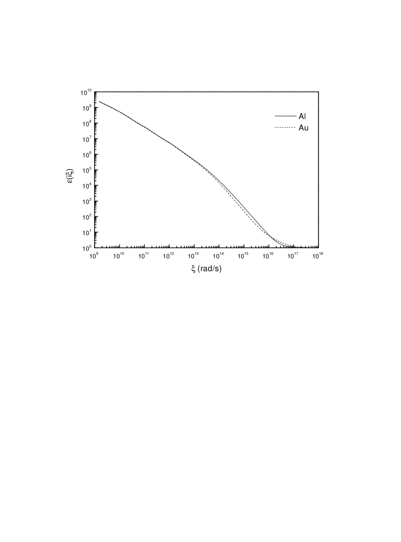
Figure 10: The dielectric permittivity as a function of imaginary frequency for $Al$ (solid line) and $Au$ (dashed line).

As is seen from Fig. 10, the dielectric permittivity along the imaginary axis decreases monotonically with increasing frequency (in distinction to Im$\varepsilon(\omega)$ which possesses peaks corresponding to interband absorption).

The obtained values of the dielectric permittivity along the imaginary axis were substituted into Eqs. (4.25) and (4.26), (4.106) to calculate the Casimir force acting between real metals in configurations of two semispaces (ss) and a sphere (lens) above a disk (dl). Numerical integration was done from an upper limit of $10^{4}\,$eV to a lower limit of $10^{-6}\,$eV. Changes in the upper limit or lower limit by a factor of 10 lead to changes of less than 0.25% in the Casimir force. If the trapezoidal rule is used in the numerical integration of Eq. (5.68) the corresponding Casimir force decreases by a factor less than 0.5%. The results are presented in Fig. 11 (two semispaces) and in Fig. 12 for a sphere above a disk by the solid lines 1 (material of the test bodies is aluminium) and 2 (material is gold).

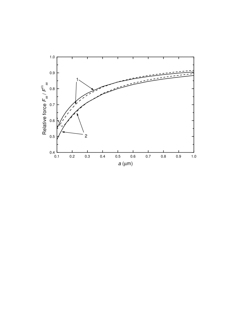
Figure 11: The correction factor to the Casimir force due to finite conductivity of the metal as a function of the surface separation in the configuration of two semispaces. The solid lines 1 and 2 represent the computational results for $Al$ and $Au$ respectively. The dashed lines 1 and 2 represent the perturbation correction factor up to the 4th order for the same metals.

In the vertical axis the relative force $F_{ss}^{C}/F_{ss}^{(0)}$ is plotted in Fig. 11 and $F_{dl}^{C}/F_{dl}^{(0)}$ in Fig. 12.

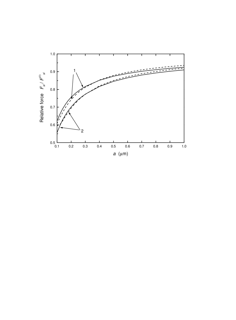
Figure 12: The correction factor to the Casimir force due to finite conductivity of the metal as a function of the surface separation for a sphere (lens) above a disk. The solid lines 1 and 2 represent the computational results for $Al$ and $Au$ respectively. The dashed lines 1 and 2 represent the perturbation correction factor up to the 4th order for the same metals.

These quantities provide a sense of the correction factors to the Casimir force due to the effect of finite conductivity. In the horizontal axis the space separation is plotted in the range 0.1–1$\,\mu$m. We do not present the results for larger distances because then the temperature corrections to the Casimir force become significant. At room temperature the temperature corrections contribute only 2.6% of $F_{dl}^{(0)}$ at $a=1\,\mu$m, but at $a=3\,\mu$m they contribute 47% of $F_{dl}^{(0)}$, and at $a=5\,\mu$m — 129% of $F_{dl}^{(0)}$ [45]. It is seen that the relative force for $Al$ is larger than for $Au$ at the same separations as it should be because of better reflectivity properties of $Al$. At the same time the relative force for $Cu$ is almost the same as for $Au$ [35].

The computational results presented here are in good agreement with analytical perturbation expansions of the Casimir force in powers of relative penetration depth of the zero-point oscillations into the metal (see the two above sections). In Fig. 11 (two semispaces) the dashed line 1 represents the results obtained by (5.60) for $Al$ with $\lambda_{p}=107\,$nm (which corresponds to $\omega_{p}=11.5\,$eV), and the dashed line 2 — the results obtained by (5.60) for $Au$ with $\lambda_{p}=136\,$nm ($\omega_{p}=9\,$eV) [35]. In Fig. 12 the dashed lines 1 and 2 represent the perturbation results obtained for $Al$ and $Au$ by (5.65) for a lens above a disk. As one can see from the figure, the perturbation results are in good (up to 0.01) agreement with computations for all distances larger than $\lambda_{p}$. Only at $a=0.1\,\mu$m for $Au$ there are larger deviations because $\lambda_{p1}\equiv\lambda_{p}^{Au}>0.1\,\mu$m. This proves the fact that the perturbation expansions (5.60) and (5.65) are applicable with rather high accuracy not for $a\gg\lambda_{p}$, as could be expected from general considerations, but for all $a\geq\lambda_{p}$.

The same formalism gives the possibility to consider the influence of thin outer metallic layers on the Casimir force value [36]. Let the semispace made of $Al$ ($\varepsilon_{2}$) be covered by $Au$ ($\varepsilon_{1}$) layers as shown in Fig. 4. For a configuration of a sphere above a plate such covering made of $Au/Pd$ was used in experiments [41, 42, 43] with different values of layer thickness $d$. In this case the Casimir force is given by the Eqs. (4.24), and (4.21), (4.106), where the quantities $Q_{1,2}(i\xi)$ are expressed by Eqs. (4.22), (4.23). The computational results for $\varepsilon(i\xi)$ are obtained from Eq. (5.68). Substituting them into (4.24) and (4.21), (4.106) and performing a numerical integration in the same way as above one obtains the Casimir force including the effect of covering layers.

The numerical computations described above show that a $Au$ layer of $d=20\,$nm thickness significantly decreases the relative Casimir force between $Al$ surfaces. With this layer the force approaches the value for pure $Au$ semispaces. For a thicker $Au$ layer of $d=30\,$nm thickness the relative Casimir force is scarcely affected by the underlying $Al$. For example, at a space separation $a=300\,$nm in the configuration of two semispaces we have $F_{ss}^{C}/F_{ss}^{(0)}=0.773$ for pure $Al$, $F_{ss}^{C}/F_{ss}^{(0)}=0.727$ for $Al$ with 20 nm $Au$ layer, $F_{ss}^{C}/F_{ss}^{(0)}=0.723$ for $Al$ with 30 nm $Au$ layer, and $F_{ss}^{C}/F_{ss}^{(0)}=0.720$ for pure $Au$. In the same way for the configuration of a sphere above a disk the results are: $F_{dl}^{C}/F_{dl}^{(0)}=0.817$ (pure $Al$), 0.780 ($Al$ with 20 nm $Au$ layer), 0.776 ($Al$ with 30 nm $Au$ layer), and 0.774 (for pure $Au$).

Let us now discuss the application range of the obtained results for the case of covering layers [36]. First, from a theoretical standpoint, the main question concerns the layer thicknesses to which the obtained formulas (4.24), and (4.21), (4.106) and the above computations can be applied. In the derivation of Sec. 4.1.1 the spatial dispersion is neglected and, as a consequence, the dielectric permittivities $\varepsilon_{\alpha}$ depend only on $\omega$ not on the wave vector $k$. In other words the field of vacuum oscillations is considered as time dependent but space homogeneous. Except for the thickness of a skin layer $\delta_{0}$ the main parameters of our problem are the velocity of the electrons on the Fermi surface, $v_{F}$, the characteristic frequency of the oscillation field, $\omega$, and the mean free path of the electrons, $l$. For the considered region of high frequencies (micrometer distances between the test bodies) the following conditions are valid [232]

$$\frac{v_{F}}{\omega}<\delta_{0}\ll l.$$ (5.70)

Note that the quantity $v_{F}/\omega$ in the left-hand side of Eq. (5.70) is the distance travelled by an electron during one period of the field, so that the first inequality is equivalent to the assumption of spatial homogeneity of the oscillating field. Usually the corresponding frequencies start from the far infrared part of spectrum, which means the space separation $a\sim 100\,\mu$m [23]. The region of high frequencies is restricted by the short-wave optical or near ultraviolet parts of the spectrum which correspond to the surface separations of several hundred nanometers. For smaller distances absorption bands, photoelectric effect and other physical phenomena should be taken into account. For these phenomena, the general Eqs. (4.24) and (4.21), (4.106), however, are still valid if one substitutes the experimental tabulated data for the dielectric permittivity along the imaginary axis incorporating all these phenomena.

Now let us include one more physical parameter — the thickness $d$ of the additional, i.e. $Au$, covering layer. It is evident that Eqs. (4.24) and (4.21), (4.106) are applicable only for layers of such thickness that

$$\frac{v_{F}}{\omega}<d.$$ (5.71)

Otherwise an electron goes out of the thin layer during one period of the oscillating field and the approximation of space homogeneity is not valid. If $d$ is so small that the inequality (5.71) is violated, the spatial dispersion should be taken into account which means that the dielectric permittivity would depend not only on frequency but on a wave vector also: $\varepsilon_{1}=\varepsilon_{1}(\omega,{\mbox{\boldmath$k$}})$. So, if (5.71) is violated, the situation is analogous to the anomalous skin effect where only space dispersion is important and the inequalities below are valid

$$\delta_{0}(\omega)<\frac{v_{F}}{\omega},\qquad\delta_{0}(\omega)<l.$$ (5.72)

In our case, however, the role of $\delta_{0}$ is played by the layer thickness $d$ (the influence of nonlocality effects on van der Waals force is discussed in [233, 234]).

From (5.70) and (5.71) it follows that for pure $Au$ layers ($\lambda_{p}\approx 136\,$nm) the space dispersion can be neglected only if $d\geq(25-30)\,$nm. For thinner layers a more general theory taking into account nonlocal effects should be developed to calculate the Casimir force. Thus for such thin layers the bulk tabulated data of the dielectric permittivity depending only on frequency cannot be used (see experimental investigation [235] demonstrating that for $Au$ the bulk values of dielectric constants can only be obtained from films whose thickness is about 30 nm or more). That is why the above calculated results for the case of $d=20\,$nm are subject to corrections due to the influence of spatial dispersion. From an experimental standpoint thin layers of order a few nm grown by evaporation or sputtering techniques are highly porous. This is particularly so in the case of sputtered coatings as shown in [236]. The nature of porosity is a function of the material and the underlying substrate. Thus it should be noted that the theory presented here which used the bulk tabulated data for $\varepsilon_{1}$ cannot be applied to calculate the influence of thin covering layers of $d=20\,$nm like those used in [34, 41] and of $d=8\,$nm used in [42, 43] on the Casimir force. The measured high transparency of such layers for the characteristic frequencies [34, 41] corresponds to a larger change of the force than what follows from Eqs. (4.24) and (4.21). This is in agreement with the above qualitative analyses.

Note that the role of spatial dispersion was neglected in [237] where the van der Waals interaction was considered between the metallic films of several nanometer thickness. According to the above considerations such neglect is unjustified. With account of spatial dispersion the Casimir attraction between a bulk conductor and a metal film deposited on a dielectric substrate was studied in [238].

As is seen from Figs. 11, 12 at room temperature the Casimir force does not follow its ideal field-theoretical expressions $F_{ss}^{(0)}$, $F_{dl}^{(0)}$. For the space separations less than $a=1\,\mu$m the corrections due to finite conductivity of the metal are rather large (thus, at $a=1\,\mu$m they are around 7–9% for a lens above a disk, and 10–12% for two semispaces; at $a=0.1\,\mu$m, around 38–44% (dl), and 45–52% (ss)). For $a>1\,\mu$m the temperature corrections increase very quickly (see Sec. 5.1). Actually, the range presented in Figs. 11, 12 is the beginning of a transition with decreasing $a$ from the Casimir force to the van der Waals force. In [36] the intermediate region is investigated in more detail for smaller $a$ and the values of $a$ are found where the pure (nonretarded) van der Waals regime described by Eq. (4.27) starts. In doing so, more exact values of the Hamaker constants for $Al$ and $Au$ were also calculated

$$H^{Al}=(3.6\pm 0.1)\times 10^{-19}\,\mbox{J},\qquad H^{Au}=(4.4\pm 0.2)\times 10^{-19}\,\mbox{J}$$ (5.73)

(see Eq. (4.28) for the determination of $H$).

5.3 Roughness corrections

The next point characterizing the real media is the imperfectness of their boundaries. In reality there are always small deviations from the perfect geometry, whether it be the two plane parallel plates or a spherical lens (sphere) situated above a plate. These deviations can be of different types. For example, plates can be under some nonzero angle to each other. In a more general way, the boundary surfaces may have a point dependent small deviations from the perfect plane, spherical or cylindrical shape. In all cases “small” means that the characteristic distortion amplitude $A$ is much less than the space separation $a$ between the two bodies. The distortion period $T$ can be much larger, of order of or much smaller compared to $a$. In the latter case one may speak about short scale distortions describing surface roughness. Some kinds of roughness can be described also by large scale distortions. Roughness is necessarily present on any real surface and contribute to the value of the Casimir force. Its contribution is rather large at $a\sim 1\,\mu$m and should be taken into account when comparing theory with experiment.

The problem of roughness corrections has long attracted the attention of researchers (see, e.g., [239, 240] where the roughness corrections to the nonretarded van der Waals force were found). In principle they can be calculated with perturbation theory based on the Green function method [96, 157]. In doing so a small parameter characterizes the deviation from the basic geometry. Also the formalism based on functional integration can be applied for this purpose [241, 242]. However, the resulting expressions turn out to be quite complicated and not very effective for specific applications. Because of this, we use here phenomenological methods of Sec.4.3 to calculate corrections to the Casimir force due to imperfectness of the boundary geometry [10, 227, 243, 244, 245, 246, 247]. As is shown below, for small deviations from the plane parallel geometry the accuracy of these methods is very high, so that obtained results are quite reliable and can be used for the interpretation of the modern precision experiments on Casimir force measuring. We consider first the configuration of two plane parallel plates and next a sphere (spherical lens) above a plate which are the two cases of experimental interest.

5.3.1 Expansion in powers of relative distortion amplitude: two semispaces

Consider two semispaces modeled by plates which are made of a material with a static dielectric permittivity $\varepsilon_{0}$ bounded by surfaces with small deviations from plane geometry. The approximate expression for the Casimir energy in this configuration is given by Eq. (4.113), where the function $\Psi$ was defined in (4.30), and we now change the notation $\varepsilon_{20}$ used in Sec.4.1.1 for $\varepsilon_{0}$.

As zeroth approximation in the perturbation theory we consider the Casimir force between the square plane plate $P_{1}$ with the sidelength $2L$ and the thickness $D$ and the other plane plate $P_{2}$, which is parallel to $P_{1}$ and has the same length and thickness. Our aim is to calculate the Casimir force between plates whose surfaces possess some small deviations from the plane geometry. Let us describe the surface of the first plate by the equation

$$z_{1}^{(s)}=A_{1}f_{1}(x_{1},y_{1})$$ (5.74)

and the surface of the second plate by

$$z_{2}^{(s)}=a+A_{2}f_{2}(x_{2},y_{2}),$$ (5.75)

where $a$ is the mean value of the distance between the plates. The values of the amplitudes are chosen in such a way that $\max\left|f_{i}(x_{i},y_{i}))\right|=1$. It is suitable to choose the zero point in the $z$-axis so that

$$\langle z_{1}^{(s)}\rangle\equiv A_{1}\langle f_{1}(x_{1},y_{1})\rangle\equiv\frac{A_{1}}{(2L)^{2}}\int\limits_{-L}^{L}dx_{1}\int\limits_{-L}^{L}dy_{1}\,f_{1}(x_{1},y_{1})=0,$$

$$\langle z_{2}^{(s)}\rangle\equiv a+A_{2}\langle f_{2}(x_{2},y_{2})\rangle=a.$$ (5.76)

We assume in our perturbation expansion that $A_{i}\ll a$, $a\ll D$, and $a\ll L$. At the same time, in all real situations, we have $a/D,\,a/L\ll A_{i}/a$, so that we are looking for the perturbation expansion in the powers of $A_{i}/a$ and in the zeroth orders in $a/D$ and $a/L$.

The non-normalized potential of one atom at a height $z_{2}$ over the plate $P_{1}$ is given by

$$U_{A}(x_{2},y_{2},z_{2})=-CN\int\limits_{-L}^{L}dx_{1}\int\limits_{-L}^{L}dy_{1}\int\limits_{-D}^{A_{1}f_{1}(x_{1},y_{1})}dz_{1}$$

$$\phantom{aaaaaaaaaaaa}\times\left[(x_{2}-x_{1})^{2}+(y_{2}-y_{1})^{2}+(z_{2}-z_{1})^{2}\right]^{-7/2},$$ (5.77)

where $C$ is an interaction constant from Eq. (4.109), $N$ is the number of atoms per unit volume of plates $P_{1}$ and $P_{2}$.

Let us calculate this expression as a series with respect to the parameter $A_{1}/z_{2}$, which is small due to $z_{2}\geq a\gg A_{1}$. In carrying out these calculations we can neglect the corrections of order of $z_{2}/L$ and $z_{2}/D$, i.e. assume that the thickness and length of the sides of the first plate are infinitely large.

The result of the expansion up to the fourth order with respect to the small parameter $A_{1}/z_{2}$ may be written in the form

$$U_{A}(x_{2},y_{2},z_{2})=-CN\left\{\frac{\pi}{10z_{2}^{4}}+\int\limits_{-L}^{L}dx_{1}\int\limits_{-L}^{L}dy_{1}\right.$$

$$\phantom{U_{A}(x_{2},y_{2},z_{2})=}\times\left[\frac{z_{2}f_{1}(x_{1},y_{1})}{X^{7/2}}\left(\frac{A_{1}}{z_{2}}\right)+\frac{7z_{2}^{3}f_{1}^{2}(x_{1},y_{1})}{2X^{9/2}}\left(\frac{A_{1}}{z_{2}}\right)^{2}\right.$$

$$\phantom{U_{A}(x_{2},y_{2},z_{2})=}+\frac{7z_{2}^{3}}{6X^{9/2}}\left(\frac{9z_{2}^{2}}{X}-1\right)f_{1}^{3}(x_{1},y_{1})\left(\frac{A_{1}}{z_{2}}\right)^{3}$$

$$\phantom{U_{A}(x_{2},y_{2},z_{2})=}\left.\left.+\frac{21z_{2}^{5}}{8X^{11/2}}\left(\frac{11z_{2}^{2}}{X}-3\right)f_{1}^{4}(x_{1},y_{1})\left(\frac{A_{1}}{z_{2}}\right)^{4}\right]\vphantom{\int\limits_{-L}^{L}}\right\},$$ (5.78)

with $X=(x_{1}-x_{2})^{2}+(y_{1}-y_{2})^{2}+z_{2}^{2}$. Here, the limit $L\to\infty$ is performed in the first item, which describes the perfect plates without deviations from planar case.

The normalized potential of the Casimir force between the plates may be obtained by the integration of Eq. (5.78) over the volume $V_{2}$ of the second plate using the boundary function $A_{2}f_{2}(x_{2},y_{2})$ and by division of the obtained result by the normalization constant $K$ from Eq. (4.112)

$$U^{R}(a)=\frac{N}{K}\int\limits_{-L}^{L}dx_{2}\int\limits_{-L}^{L}dy_{2}\int\limits_{a+A_{2}f_{2}(x_{2},y_{2})}^{a+D}dz_{2}\,U_{A}(x_{2},y_{2},z_{2}).$$ (5.79)

The Casimir force between the plates per unit area is given by

$$F_{ss}^{R}(a)=-\frac{1}{(2L)^{2}}\frac{\partial U^{R}(a)}{\partial a}.$$ (5.80)

Substituting (5.79) into (5.80) we can write

$$F_{ss}^{R}(a)=-\frac{1}{(2L)^{2}}\frac{N}{K}\int\limits_{-L}^{L}dx_{2}\int\limits_{-L}^{L}dy_{2}U_{A}\left[x_{2},y_{2},a+A_{2}f_{2}(x_{2},y_{2})\right].$$ (5.81)

Let us now represent the quantity $U_{A}$ defined in Eq. (5.78) as a series up to the fourth order in the small parameter $A_{2}/a$. Then we substitute this series into Eq. (5.81). The result may be written in the form

$$F_{ss}^{R}(a)=F_{ss}(a)\sum\limits_{k=0}^{4}\sum\limits_{l=0}^{4-k}c_{kl}\left(\frac{A_{1}}{a}\right)^{k}\left(\frac{A_{2}}{a}\right)^{l},$$ (5.82)

where $F_{ss}(a)$ is as defined in Eq. (4.29) in the case of perfect plates. For the coefficients in (5.82) we note that

$$c_{00}=1,\qquad c_{01}=c_{10}=0.$$ (5.83)

The last two equalities follow from the choice (5.76).

The coefficients whose first index is zero are

$$c_{02}=10\,\langle f_{2}^{2}\rangle,\qquad c_{03}=-20\,\langle f_{2}^{3}\rangle,\qquad c_{04}=35\,\langle f_{2}^{4}\rangle,$$ (5.84)

where the notation for the averaged values are used as in Eq. (5.76).

The remaining coefficients $c_{kl}$ in Eq. (5.82) are more complicated. They read

$$c_{20}=\frac{35}{\pi}a^{7}\langle f_{1}^{2}Y^{-9}\rangle,\qquad c_{30}=\frac{35}{\pi}a^{7}\langle f_{1}^{3}\varphi_{1}(Y)\rangle,$$

$$c_{40}=\frac{105}{4\pi}a^{9}\langle f_{1}^{4}\varphi_{2}(Y)\rangle,\qquad c_{11}=-\frac{70}{\pi}a^{7}\langle f_{1}f_{2}Y^{-9}\rangle,$$

$$c_{12}=\frac{35}{\pi}a^{7}\langle f_{1}f_{2}^{2}\varphi_{1}(Y)\rangle,\qquad c_{21}=-\frac{35}{\pi}a^{7}\langle f_{1}^{2}f_{2}\varphi_{1}(Y)\rangle,$$ (5.85)

$$c_{13}=-\frac{105}{\pi}a^{9}\langle f_{1}f_{2}^{3}\varphi_{2}(Y)\rangle,\qquad c_{31}=-\frac{105}{\pi}a^{9}\langle f_{1}^{3}f_{2}\varphi_{2}(Y)\rangle,$$

$$c_{22}=\frac{315}{\pi}a^{9}\langle f_{1}^{2}f_{2}^{2}\varphi_{2}(Y)\rangle.$$

In (5.85) the following notations are used

$$Y=\left[(x_{1}-x_{2})^{2}+(y_{1}-y_{2})^{2}+a^{2}\right]^{1/2},$$ (5.86)

$$\varphi_{1}(Y)=9a^{2}Y^{-11}-Y^{-9},\quad\varphi_{2}(Y)=11a^{2}Y^{-13}-3Y^{-11},$$

and the following averaging procedure for a function depending on four variables

$$\langle\Phi(x_{1},y_{1};x_{2},y_{2})\rangle=\frac{1}{(2L)^{2}}\int\limits_{-L}^{L}dx_{2}\int\limits_{-L}^{L}dy_{2}\int\limits_{-L}^{L}dx_{1}\int\limits_{-L}^{L}dy_{1}\Phi(x_{1},y_{1};x_{2},y_{2}).$$ (5.87)

We have also used the notations $f_{1}\equiv f_{1}(x_{1},y_{1})$, $f_{2}\equiv f_{2}(x_{2},y_{2})$.

To obtain the general result for corrections to the Casimir force, we need to calculate the values of the coefficients $c_{lk}$ defined in (5.85). We start with the coefficients $c_{l0}$ which depend on one distortion function only. Integrating over $x_{2}$ and $y_{2}$ according to (5.87) from $-\infty$ to $\infty$, we obtain to zeroth order in $a/L$

$$c_{20}=10\,\langle f_{1}^{2}\rangle,\qquad c_{30}=20\,\langle f_{1}^{3}\rangle,\qquad c_{40}=35\,\langle f_{1}^{4}\rangle.$$ (5.88)

These results are in agreement with Eq. (5.84) and may be obtained also from symmetry considerations.

The calculation of the mixed coefficients (depending on the deviation functions of both plates) is quite complicated. The results read [10]

$$c_{11}=-\frac{4}{3}\sqrt{\frac{2}{\pi}}\sum\limits_{m=0}^{\infty}\sum\limits_{n=0}^{\infty}G_{mn}^{(1,1)}z_{mn}^{7/2}K_{7/2}(z_{mn}),$$

$$c_{12}=\frac{2}{3}\sqrt{\frac{2}{\pi}}\sum\limits_{m=0}^{\infty}\sum\limits_{n=0}^{\infty}G_{mn}^{(1,2)}z_{mn}^{7/2}\left[z_{mn}K_{9/2}(z_{mn})-K_{7/2}(z_{mn})\right],$$ (5.89)

$$c_{13}=-\frac{2}{9}\sqrt{\frac{2}{\pi}}\sum\limits_{m=0}^{\infty}\sum\limits_{n=0}^{\infty}G_{mn}^{(1,3)}z_{mn}^{9/2}\left[z_{mn}K_{11/2}(z_{mn})-K_{9/2}(z_{mn})\right],$$

$$c_{22}=210g_{00}^{(2)}h_{00}^{(2)}+\frac{1}{3}\sqrt{\frac{2}{\pi}}\sum\limits_{m=0}^{\infty}\sum\limits_{n=0}^{\infty}G_{mn}^{(2,2)}z_{mn}^{9/2}\left[z_{mn}K_{11/2}(z_{mn})-K_{9/2}(z_{mn})\right].$$

Let us explain the notations in Eqs. (5.89). The functions $K_{\nu}(z)$ are the modified Bessel functions,

$$z_{mn}\equiv\pi\frac{a}{L}\sqrt{n^{2}+m^{2}}.$$ (5.90)

The quantities $G_{mn}^{(i,k)}$ are given by

$$G_{mn}^{(i,k)}=\frac{1}{4}\left(1+\delta_{m0}+\delta_{n0}\right)\sum\limits_{l=1}^{4}g_{l,mn}^{(i)}h_{l,mn}^{(k)},$$ (5.91)

where $\delta_{m0}$ is the Kronecker symbol and $g_{l,mn}^{(i)}$ and $h_{l,mn}^{(k)}$ are the Fourier coefficients of the functions $f_{1}^{i}$ and $f_{2}^{k}$, considered as periodic functions with the period $2L$ (for details see [10]). The quantities $g_{00}^{(2)}$ and $h_{00}^{(2)}$ are the zeroth terms of the Fourier expansions of the functions $f_{1}^{2}$ and $f_{2}^{2}$ respectively. The coefficient $c_{21}$ differs from $c_{12}$ by its sign and by the sequence of upper indices of $G$. For obtaining of $c_{31}$ it is enough just to change the sequence of upper indices of $G$ in $c_{13}$.

So, the perturbation formalism developed allows one to obtain the Casimir force for configurations with deviations from plane parallel geometry in the form of the series, given by Eq. (5.82), with coefficients defined in Eqs. (5.83), (5.84), (5.88) and (5.89). These coefficients can be calculated explicitly for various kinds of distortions. However, the simple case of nonparallel plates is of prime interest here because an exact Casimir force value is also known for it. This gives the possibility to estimate the accuracy of the above phenomenological approach.

5.3.2 Casimir force between nonparallel plates and plates covered by large scale distortions

Let us consider the Casimir force for the configuration of two plane plates with angle $\alpha$ between them. This angle is assumed to be small, so that the inequality $\alpha L\ll a$ holds. This configuration is a particular example for the deviation from plane parallel geometry which a characteristic length scale is much larger than $a$. For all deviations of such kind the coefficients (5.89) can be calculated in a general form. To do this we use the explicit expressions of the modified Bessel functions [226] in (5.89) and obtain [10]

$$c_{11}=-20\sum\limits_{m=0}^{\infty}\sum\limits_{n=0}^{\infty}G_{mn}^{(1,1)}e^{-z_{mn}}\left(1+z_{mn}+\frac{2}{5}z_{mn}^{2}+\frac{1}{15}z_{mn}^{3}\right),$$

$$c_{12}=60\sum\limits_{m=0}^{\infty}\sum\limits_{n=0}^{\infty}G_{mn}^{(1,2)}e^{-z_{mn}}\left(1+z_{mn}+\frac{13}{30}z_{mn}^{2}+\frac{1}{10}z_{mn}^{3}+\frac{1}{90}z_{mn}^{4}\right),$$

$$c_{13}=-140\sum\limits_{m=0}^{\infty}\sum\limits_{n=0}^{\infty}G_{mn}^{(1,3)}e^{-z_{mn}}\left[1+z_{mn}\Pi(z_{mn})\right],$$ (5.92)

$$c_{22}=210\left\{g_{00}^{(2)}h_{00}^{(2)}+\sum\limits_{m=0}^{\infty}\sum\limits_{n=0}^{\infty}G_{mn}^{(2,2)}e^{-z_{mn}}\left[1+z_{mn}\Pi(z_{mn})\right]\right\},$$

where $\Pi(z)=1+\frac{19}{42}z+\frac{5}{42}z^{2}+\frac{2}{105}z^{3}+\frac{1}{630}z^{4}$.

The Fourier coefficients of the distortion functions $f_{1,2}$ and their powers decrease quickly with the number of harmonics. Due to Eq. (5.91) the quantities $G_{mn}^{(i,k)}$ also decrease with the increase in $m$ and $n$. The quantity $z_{mn}$, defined in (5.90), is of order of $a/L\ll 1$ for all harmonics which give a significant contribution to the coefficients $c_{ik}$. So, we can put in Eq. (5.92) $z_{mn}=0$ without loss of accuracy:

$$c_{11}=-20\sum\limits_{m=0}^{\infty}\sum\limits_{n=0}^{\infty}G_{mn}^{(1,1)},\qquad c_{12}=60\sum\limits_{m=0}^{\infty}\sum\limits_{n=0}^{\infty}G_{mn}^{(1,2)},$$

$$c_{13}=-140\sum\limits_{m=0}^{\infty}\sum\limits_{n=0}^{\infty}G_{mn}^{(1,3)},$$ (5.93)

$$c_{22}=210\left(g_{00}^{(2)}h_{00}^{(2)}+\sum\limits_{m=0}^{\infty}\sum\limits_{n=0}^{\infty}G_{mn}^{(2,2)}\right).$$

Taking into account Eq. (5.91) and the elementary properties of Fourier expansions, it is possible to rewrite Eqs. (5.93) in the form

$$c_{11}=-20\langle f_{1}f_{2}\rangle,\qquad c_{12}=60\langle f_{1}f_{2}^{2}\rangle,$$

$$c_{13}=-140\langle f_{1}f_{2}^{3}\rangle,\qquad c_{22}=210\langle f_{1}^{2}f_{2}^{2}\rangle,$$ (5.94)

$$c_{21}=-60\langle f_{1}^{2}f_{2}\rangle,\qquad c_{31}=-140\langle f_{1}^{3}f_{2}\rangle$$

(in the last line the correlations between $c_{ik}$ and $c_{ki}$ have been used — see Sec.5.3.1).

By the use of Eqs. (5.83), (5.84), (5.88) and (5.94) the final result for the Casimir force from Eq. (5.82) can be represented in the form [10]

$$F_{ss}^{R}(a)=F_{ss}(a)\left\{1+10\left[\langle f_{1}^{2}\rangle\left(\frac{A_{1}}{a}\right)^{2}-2\langle f_{1}f_{2}\rangle\left(\frac{A_{1}}{a}\right)\left(\frac{A_{2}}{a}\right)+\langle f_{2}^{2}\rangle\left(\frac{A_{2}}{a}\right)^{2}\right]\right.$$

$$\phantom{F_{ss}^{R}(a)=}+20\left[\langle f_{1}^{3}\rangle\left(\frac{A_{1}}{a}\right)^{3}-3\langle f_{1}^{2}f_{2}\rangle\left(\frac{A_{1}}{a}\right)^{2}\left(\frac{A_{2}}{a}\right)\right.$$

$$\phantom{F_{ss}^{R}(a)=}+\left.3\langle f_{1}f_{2}^{2}\rangle\left(\frac{A_{1}}{a}\right)\left(\frac{A_{2}}{a}\right)^{2}-\langle f_{2}^{3}\rangle\left(\frac{A_{2}}{a}\right)^{3}\right]$$

$$\phantom{F_{ss}^{R}(a)=}+35\left[\langle f_{1}^{4}\rangle\left(\frac{A_{1}}{a}\right)^{4}-4\langle f_{1}^{3}f_{2}\rangle\left(\frac{A_{1}}{a}\right)^{3}\left(\frac{A_{2}}{a}\right)+6\langle f_{1}^{2}f_{2}^{2}\rangle\left(\frac{A_{1}}{a}\right)^{2}\left(\frac{A_{2}}{a}\right)^{2}\right.$$

$$\phantom{F_{ss}^{R}(a)=}-\left.\left.4\langle f_{1}f_{2}^{3}\rangle\left(\frac{A_{1}}{a}\right)\left(\frac{A_{2}}{a}\right)^{3}+\langle f_{2}^{4}\rangle\left(\frac{A_{2}}{a}\right)^{4}\right]\right\}.$$ (5.95)

As can be seen from Eq. (5.95), the mixed terms have an evident interference character. For example, in the particular case $f_{2}=\mp f_{1}$ we have

$$F_{ss}^{R}(a)=F_{ss}(a)\left[1+10\langle f_{1}^{2}\rangle\left(\frac{A_{1}}{a}\pm\frac{A_{2}}{a}\right)^{2}+20\langle f_{1}^{3}\rangle\left(\frac{A_{1}}{a}\pm\frac{A_{2}}{a}\right)^{3}\right.$$

$$\phantom{aaaaaaaaaaa}\left.+35\langle f_{1}^{4}\rangle\left(\frac{A_{1}}{a}\pm\frac{A_{2}}{a}\right)^{4}\right].$$ (5.96)

Now, let us apply the results (5.95) and (5.96) to the case of two plane plates with a small angle $\alpha$ between them. This configuration can be realized in three ways. For example, the upper plate may be left flat and the lower plate allowed to deviate from the parallel position as described by the function

$$f_{1}(x_{1},y_{1})=\frac{x_{1}}{l}$$ (5.97)

with the amplitude $A_{1}=\alpha L$. Substituting (5.97) into the expression (5.95) for the Casimir force and putting $A_{2}=0$, one obtains

$$F_{ss}^{R}(a)=F_{ss}(a)\left[1+10\langle f_{1}^{2}\rangle\left(\frac{A_{1}}{a}\right)^{2}+20\langle f_{1}^{3}\rangle\left(\frac{A_{1}}{a}\right)^{3}+35\langle f_{1}^{4}\rangle\left(\frac{A_{1}}{a}\right)^{4}\right].$$ (5.98)

Using the averaged values calculated from the function (5.97), one further obtains

$$F_{ss}^{R}(a)=F_{ss}(a)\left[1+\frac{10}{3}\left(\frac{\alpha L}{a}\right)^{2}+7\left(\frac{\alpha L}{a}\right)^{4}\right].$$ (5.99)

The same configuration can be obtained in a way when both plates are perturbed with the amplitudes $A_{1}=\alpha_{1}L$ and $A_{2}=\alpha_{2}L$. The angle between them is, thereby, $\alpha=\alpha_{1}+\alpha_{2}$ or $\alpha=|\alpha_{1}-\alpha_{2}|$ and the deviation functions are given by Eq. (5.97) supplemented by $f_{2}=\mp f_{1}$ respectively.

It is easy to see that the calculation of the Casimir force according to Eq. (5.96) repeats the result (5.99). This example is interesting, because it gives the possibility of observing the role of the interference terms in (5.95). Such terms must be taken into account in order to obtain the proper result.

The configuration of two nonparallel plates can also be considered by the method of Green functions. For this purpose let us use the exact expression for the Casimir energy density of electromagnetic field inside a wedge obtained by this method in [215, 248]

$${{E}}(\rho)=-\frac{(n^{2}-1)(n^{2}+11)}{720\pi^{2}\rho^{4}},$$ (5.100)

where $\rho$ is the distance from the line of intersection of the wedge faces, and $n=\pi/\alpha$.

The total energy in the space between two square plates of side length $2L=\rho_{2}-\rho_{1}$ at an angle $\alpha$ to each other is

$$U^{R}=\int\limits_{0}^{\alpha}d\varphi\int\limits_{0}^{2L}dz\int\limits_{\rho_{1}}^{\rho_{2}}d\rho\,\rho{E}(\rho).$$ (5.101)

Substituting Eq. (5.100) into Eq. (5.101) and integrating, keeping $\alpha\ll 1$, one obtains the result

$$U^{R}=U^{R}(a)=-\frac{\pi^{2}L}{720\alpha}\left[\frac{1}{(a-\alpha L)^{2}}-\frac{1}{(a+\alpha L)^{2}}\right],$$ (5.102)

where $a$ is the mean distance between the two plates.

Then the Casimir force can be obtained from Eq. (5.80) as

$$F_{ss}^{R}(a)=-\frac{\pi^{2}}{1440\alpha L}\left[\frac{1}{(a-\alpha L)^{3}}-\frac{1}{(a+\alpha L)^{3}}\right].$$ (5.103)

Expanding this expression for the force as a series with respect to powers of the small parameter $\alpha L/a$ up to fourth order, one exactly obtains Eq. (5.99).

So it has been shown that, at least up to the fourth order inclusive in the parameter $\alpha L/a$, the approximate approach based on the additive summation with a subsequent normalization yields exactly the same result as the Green function method if the slope angle between plates is small. This allows to make an estimate of the relative error of the above approach used for configurations with small deviations from the plane parallel geometry. Taking the realistic estimation of $\alpha L/a\approx 10^{-1}$, the conclusion is obtained that the relative error of the result (5.95) for the Casimir force is much less than $10^{-2}$%. Therefore, the application of the approach under consideration to configurations with small deviations from plane parallel geometry can be expected to give reliable results up to the fourth order in the parameter $A_{1,2}/a$.

As was noted above, the Eq. (5.95) is valid for any large scale distortions whose characteristic length scale $T\gg a$. Such distortions may describe large scale surface roughness. Let us consider the longitudinal distortions with amplitudes $A_{1,2}$ described by the functions

$$f_{1}(x_{1},y_{1})=\sin\omega x_{1},\qquad f_{2}(x_{2},y_{2})=\sin(\omega x_{2}+\delta).$$ (5.104)

In the case when $\omega^{-1}\ll L$ the mean values of the functions $f_{1,2}^{k}$ in Eq. (5.95) can be calculated as the mean values for one period. Substituting these results into Eq. (5.95), one obtains [10]

$$F_{ss}^{R}(a)=F_{ss}(a)\left\{1+5\left[\left(\frac{A_{1}}{a}\right)^{2}-2\cos\delta\left(\frac{A_{1}}{a}\right)\left(\frac{A_{2}}{a}\right)+\left(\frac{A_{2}}{a}\right)^{2}\right]\right.$$

$$\phantom{F_{ss}^{R}(a)=}+\frac{105}{8}\left[\left(\frac{A_{1}}{a}\right)^{4}-4\cos\delta\left(\frac{A_{1}}{a}\right)^{3}\left(\frac{A_{2}}{a}\right)\right.$$ (5.105)

$$\phantom{F_{ss}^{R}(a)=}+2(2+\cos 2\delta)\left(\frac{A_{1}}{a}\right)^{2}\left(\frac{A_{2}}{a}\right)^{2}-\left.\left.4\cos\delta\left(\frac{A_{1}}{a}\right)\left(\frac{A_{2}}{a}\right)^{3}+\left(\frac{A_{2}}{a}\right)^{4}\right]\right\}.$$

It is seen that the result depends significantly on the value of phase shift $\delta$.

If the periods of the distortion functions in Eq. (5.104) are different, it is necessary to calculate the mean values in the mixed terms over the whole plate according to Eq. (5.76). It can be seen that in this case only the contribution of $\langle f_{1}^{2}f_{2}^{2}\rangle=1/4$ to the mixed terms is not equal to zero. So, the Casimir force is

$$F_{ss}^{R}(a)=F_{ss}(a)\left\{1+5\left[\left(\frac{A_{1}}{a}\right)^{2}+\left(\frac{A_{2}}{a}\right)^{2}\right]\right.$$ (5.106)

$$\phantom{F_{ss}^{R}(a)=}+\frac{105}{8}\left.\left[\left(\frac{A_{1}}{a}\right)^{4}+4\left(\frac{A_{1}}{a}\right)^{2}\left(\frac{A_{2}}{a}\right)^{2}+\left(\frac{A_{2}}{a}\right)^{4}\right]\right\}.$$

The force from Eq. (5.106) is evidently larger than the force from Eq. (5.105) for $\delta=0$, but smaller than that for $\delta=\pi$.

5.3.3 Casimir force between plates covered by short-scale roughness

The surfaces of real plates are always covered by some short scale distortions or short scale roughness of different types. It is necessary to take into account the contribution of such distortions in precision experiments on Casimir force measurements. The characteristic longitudinal scales of such distortions are of order (or less than) the distance $a$ between plates.

The distortions of the plate surfaces may be periodic or nonperiodic. In both cases the general result for the Casimir force (see Eq. (5.82) with the coefficients (5.83), (5.84), (5.88) and (5.92)) acquires one and the same, simpler form than those presented by Eq. (5.95). As we shall see below, most of the mixed terms in Eq. (5.82) turn into zero for the short scale distortions. The reasons for such simplifications are different for the cases of periodic and nonperiodic distortions. Let us start with the nonperiodic case, which is the more general.

If the functions $f_{1,2}$ are nonperiodic, the result (5.95) for the Casimir force applies. Because the characteristic scale of the distortions is of the order $a\ll L$, and by means of Eq. (5.76), we obtain for the odd numbers ($i,k$)

$$\langle f_{1}^{i}f_{2}^{k}\rangle=0.$$ (5.107)

By the use of this, Eq. (5.95) takes the form

$$F_{ss}^{R}(a)=F_{ss}(a)\left\{1+10\left[\langle f_{1}^{2}\rangle\left(\frac{A_{1}}{a}\right)^{2}+\langle f_{2}^{2}\rangle\left(\frac{A_{2}}{a}\right)^{2}\right]\right.$$ (5.108)

$$\phantom{F_{ss}^{R}(a)=}+35\left.\left[\langle f_{1}^{4}\rangle\left(\frac{A_{1}}{a}\right)^{4}+6\langle f_{1}^{2}f_{2}^{2}\rangle\left(\frac{A_{1}}{a}\right)^{2}\left(\frac{A_{2}}{a}\right)^{2}+\langle f_{2}^{4}\rangle\left(\frac{A_{2}}{a}\right)^{4}\right]\right\}.$$

The same result occurs for large scale periodic distortions with different periods.

Now, let the functions $f_{1,2}$ be periodic. If the periods of $f_{1}$ and $f_{2}$ are different (at least in one coordinate), Eq. (5.107) is valid once more and we return to the expression (5.108) for the Casimir force.

A different formula appears only in the case when periods $T_{x}$ and $T_{y}$ of $f_{1}$ and $f_{2}$ are equal in both coordinates respectively. It is evident in our case that $2L\approx mT_{x}$, $2L\approx nT_{y}$ holds where $m,\,n\gg 1$. In the Fourier expansions of the functions $f_{1}^{i}$ and $f_{2}^{k}$ the coefficients of the modes with the corresponding large numbers are large. So, in Eq. (5.92) the main contributions are given by the terms containing the coefficients $G_{mn}^{(i,k)}$, which were defined in Eq. (5.91), with $m,\,n$ large. The parameter $z_{mn}$ defined in Eq. (5.90) is of the order of $a/T_{x,y}$ in that case.

For extremely short scale distortions $T_{x,y}\ll a$ we have $e^{-z_{mn}}\to 0$ and only one coefficient among all the mixed ones survives:

$$c_{22}=210g_{00}^{(2)}h_{00}^{(2)}\equiv 210\langle f_{1}^{2}\rangle\langle f_{2}^{2}\rangle.$$ (5.109)

As a consequence the Casimir force for the extremely short scale distortions has the form [10]

$$F_{ss}^{R}(a)=F_{ss}(a)\left\{1+10\left[\langle f_{1}^{2}\rangle\left(\frac{A_{1}}{a}\right)^{2}+\langle f_{2}^{2}\rangle\left(\frac{A_{2}}{a}\right)^{2}\right]\right.$$ (5.110)

$$\phantom{F_{ss}^{R}(a)=}+35\left.\left[\langle f_{1}^{4}\rangle\left(\frac{A_{1}}{a}\right)^{4}+6\langle f_{1}^{2}\rangle\langle f_{2}^{2}\rangle\left(\frac{A_{1}}{a}\right)^{2}\left(\frac{A_{2}}{a}\right)^{2}+\langle f_{2}^{4}\rangle\left(\frac{A_{2}}{a}\right)^{4}\right]\right\}.$$

For the case $T_{x,y}\sim a$ one should calculate the coefficients of Eq. (5.92) according to nonsimplified formulas.

As an example of periodic distortions let us examine the longitudinal ones described by Eq. (5.104) with $\omega^{-1}\sim a$. Calculating the mixed coefficients according to Eq. (5.92) and taking into account that only $G_{m,0}=1$ with $m=\omega L/\pi$ is not equal to zero, one obtains

$$c_{11}=-20\cos\delta e^{-z_{m0}}\left[1+z_{m0}+\frac{2}{5}(z_{m0})^{2}+\frac{1}{15}(z_{m0})^{3}\right],$$

$$c_{12}=c_{21}=0,$$ (5.111)

$$c_{13}=c_{31}=-\frac{105}{2}\cos\delta\,e^{-z_{m0}}\left[1+z_{m0}\Pi(z_{m0})\right],$$

$$c_{22}=\frac{105}{2}\left\{1+\cos 2\delta\,e^{-z_{m0}}\left[1+z_{m0}\Pi(z_{m0})\right]\right\},$$

where $\Pi(z)$ is as defined in Eq. (5.92) and $z_{m0}=\omega a$.

If $\omega a\gg 1$, the terms of Eq. (5.111) containing the exponential factors can be neglected and we return to the result (5.110) with

$$\langle f_{1}^{2}\rangle=\langle f_{2}^{2}\rangle=\frac{1}{2},\qquad\langle f_{1}^{4}\rangle=\langle f_{2}^{4}\rangle=\frac{3}{8}.$$ (5.112)

It is seen that this result coincides with (5.106) and does not depend on the phase shift $\delta$ as would be expected in this case.

For $\omega^{-1}\sim a$ one ought to make computations. For example, for $z_{m0}=1$ the results are

$$c_{11}=-18.08\cos\delta,\qquad c_{13}=-49.98\cos\delta,$$

$$c_{22}=\frac{105}{2}(1+0.953\cos 2\delta).$$ (5.113)

The other coefficients coincide with those obtained in Sec.5.3.2 for this example. They are contained in Eq. (5.105) and do not depend on the period. The detailed investigation of the transition region between the large scale and short scale roughness is contained in [246].

Substituting all these coefficients into Eq. (5.82), one obtains the Casimir force which is analogous to Eq. (5.105) for larger periods. It is seen that under a decrease of the period the absolute values of the coefficients of the interference terms, i.e. the terms, containing $\delta$, decrease [10].

In the above manner, the Casimir force between the plates covered by all types of small distortions can be described perturbatively with a required accuracy (note that the case of an atom near the cavity wall covered by roughness is examined in detail in [247]).

5.3.4 Expansion in powers of relative distortion amplitude: a spherical lens above a plate

The configuration of a spherical lens (or a sphere) above a plate (or a disk) is the most preferable from the experimental point of view (see Sec.6). Because of this a knowledge of roughness corrections in this configuration is necessary to compare theoretical predictions with the results of the Casimir force measurements. Let us start from the same approximate expression for the Casimir force potential as for two plates given by Eqs. (4.113), (4.30). Let the lens curvature radius be $R$, thickness $h$, diameter $2r$. The parameters of a plate are the same as in Sec.5.3.1. The coordinate plane ($x,\,y$) is chosen to coincide with the plate surface.

As above, the surface of the plate with some small distortions can be described by Eq. (5.74) with a condition given by the first equality of (5.76). Let us consider the surface of a lens with small deviations from the ideal spherical shape described by the equation

$$z_{2}^{(s)}=a+R-\sqrt{R^{2}-\rho^{2}}+A_{2}f_{2}(\rho,\varphi),$$ (5.114)

where $\rho,\,\varphi$ are the polar coordinates. The perturbation theory can be developed in the same way as in Sec.5.3.1. As a result the normalized potential of the Casimir force acting between the lens and the plate is given by

$$U^{R}(a)=-\hbar c\Psi(\varepsilon)\int\limits_{0}^{2\pi}d\varphi\int\limits_{0}^{r}\rho d\rho\int\limits_{z_{2}^{(s)}}^{h+a}dz_{2}U_{A}(\rho,\varphi,z_{2}),$$ (5.115)

where

$$U_{A}(\rho,\varphi,z_{2})=\int\limits_{-L}^{L}dx_{1}\int\limits_{-L}^{L}dy_{1}\int\limits_{-D}^{z_{1}^{(s)}}dz_{1}$$ (5.116)

$$\phantom{U_{A}(\rho,\varphi,z_{2})=}\times\left[(x_{1}-\rho\cos\varphi)^{2}+(y_{1}-\rho\sin\varphi)^{2}+(z_{1}-z_{2})^{2}\right]^{-7/2}.$$

The function (5.116) was calculated in Sec.5.3.1 as a series with respect to the parameter $A_{1}/z_{2}$, which is small due to $z_{2}>a\gg A_{1}$. Neglecting the corrections of the order of $z_{2}/L$ and $z_{2}/D$ one has

$$U_{A}(\rho,\varphi,z_{2})=\frac{\pi}{10z_{2}^{4}}+\int\limits_{-L}^{L}dx_{1}\int\limits_{-L}^{L}dy_{1}$$ (5.117)

$$\phantom{U_{A}(\rho,\varphi,z_{2})=}\times\left[z_{2}f_{1}(x_{1},y_{1})X^{-7/2}\left(\frac{A_{1}}{z_{2}}\right)+\frac{7}{2}z_{2}^{3}f_{1}^{2}(x_{1},y_{1})X^{-9/2}\left(\frac{A_{1}}{z_{2}}\right)^{2}\right],$$

with $X=(x_{1}-\rho\cos\varphi)^{2}+(y_{1}-\rho\sin\varphi)^{2}+z_{2}^{2}$. Here the limiting transition $L\to\infty$ is performed in the first item, which describes the contribution of the perfect plate without deviations from the plane. For brevity we restrict ourselves to second order perturbation.

Substituting Eq. (5.117) in Eq. (5.115) and calculating force as $-\partial U^{R}/\partial a$, we arrive to the result in zeroth order with respect to the small parameter $a/h$

$$F_{dl}^{R}(a)=-\hbar c\Psi(\varepsilon)\int\limits_{0}^{2\pi}d\varphi\int\limits_{0}^{r}\rho\,d\rho U_{A}(\rho,\varphi,z_{2}^{(s)}).$$ (5.118)

Here $z_{2}^{(s)}$ is as defined by Eq. (5.114).

Let us now represent the quantity $U_{A}(\rho,\varphi,z_{2}^{(s)})$ in Eq. (5.118) as a series up to the second order in the small parameter $A_{2}/a$. After integration, the result can be written in the form

$$F_{dl}^{R}(a)=F_{dl}(a)\sum\limits_{k=0}^{2}\sum\limits_{l=0}^{2-k}C_{kl}\left(\frac{A_{1}}{a}\right)^{k}\left(\frac{A_{2}}{a}\right)^{l},$$ (5.119)

where $F_{dl}(a)$ is defined by Eq. (4.115). For the first coefficient in Eq. (5.119) we note that

$$C_{00}=1.$$ (5.120)

The other coefficients in Eq. (5.119) in zeroth order with respect to small parameters $a/h$, $a/r$, $r/R$, $a/L$ are [245]

$$C_{01}=-\frac{6}{\pi Ra}\int\limits_{0}^{2\pi}d\varphi\int\limits_{0}^{\infty}\rho d\rho f_{2}(\rho,\varphi)\,\left(1+\frac{\rho^{2}}{2aR}\right)^{-5},$$

$$C_{02}=\frac{15}{\pi Ra}\int\limits_{0}^{2\pi}d\varphi\int\limits_{0}^{\infty}\rho d\rho f_{2}^{2}(\rho,\varphi)\,\left(1+\frac{\rho^{2}}{2aR}\right)^{-6},$$

$$C_{10}=\frac{15a^{4}}{\pi^{2}R}\langle f_{1}Y^{-7}\rangle,$$ (5.121)

$$C_{20}=\frac{105a^{5}}{2\pi^{2}R}\langle f_{1}^{2}\left(a+\frac{\rho^{2}}{2R}\right)Y^{-9}\rangle,$$

$$C_{11}=-\frac{105a^{5}}{2\pi^{2}R}\langle f_{1}f_{2}\left(a+\frac{\rho^{2}}{2R}\right)Y^{-9}\rangle.$$

In Eqs. (5.121) we use the notation

$$Y=\left[(x_{1}-\rho\cos\varphi)^{2}+(y_{1}-\rho\sin\varphi)^{2}+\left(a+\frac{\rho^{2}}{2R}\right)^{2}\right]^{1/2}$$ (5.122)

and the following avaraging procedure for a function depending on four variables

$$\langle\Phi(\rho,\varphi;x_{1},y_{1})\rangle=\int\limits_{0}^{2\pi}d\varphi\int\limits_{0}^{\infty}\rho d\rho\int\limits_{-\infty}^{\infty}dx_{1}\int\limits_{-\infty}^{\infty}dy_{1}\Phi(\rho,\varphi;x_{1},y_{1}).$$ (5.123)

Besides, we have used in Eqs. (5.121) the notations $f_{1}\equiv f_{1}(x_{1},y_{1})$, $f_{2}\equiv f_{2}(\rho,\varphi)$. A point that should be mentioned is that the coefficients $C_{01}$, $C_{10}$ in Eq. (5.119) in general differ from zero. For the configuration of two parallel plates with small distortions, the analogical perturbative expansion starts from the second order (see Sec.5.3.1).

The coefficients given by Eqs. (5.121), and also the ones of higher orders, can be calculated in the same way as illustrated in Secs.5.3.1, 5.3.2 for the example of two plates. For this purpose the distortion function $f_{1}$ is considered as a periodic one with a period $2L$ in both variables and the function $f_{2}(\rho,\varphi)$ is considered as a periodic function of $\rho$ with a period $r$. All the details can be found in Ref. [245]. Instead of presenting the detailed algebra, here we only discuss the specific results which are applicable to experiments.

5.3.5 Corrections to the Casimir force between a plate and a lens due to different kinds of roughness

Let us consider first the short scale roughness on the plate (disk) and on the lens with characteristic longitudinal scales $T_{d}$, $T_{l}$ which are the subject to the inequality

$$T_{d},\,T_{l}\ll\sqrt{aR}.$$ (5.124)

In this case only the terms of the Fourier expansions of the functions $f_{1}^{i}$, $f_{2}^{k}$ with sufficiently large numbers are significant. As a result all the expansion coefficients from Eq. (5.119) can be calculated in a closed form. The result up to the fourth order in the relative roughness amplitude is

$$F_{dl}^{R}(a)=F_{dl}(a)\left\{1+6\left[\langle f_{1}^{2}\rangle\left(\frac{A_{1}}{a}\right)^{2}-2\langle f_{1}f_{2}\rangle\left(\frac{A_{1}}{a}\right)\left(\frac{A_{2}}{a}\right)+\langle f_{2}^{2}\rangle\left(\frac{A_{2}}{a}\right)^{2}\right]\right.$$

$$\phantom{F_{ss}^{R}(a)=}+10\left[\langle f_{1}^{3}\rangle\left(\frac{A_{1}}{a}\right)^{3}-3\langle f_{1}^{2}f_{2}\rangle\left(\frac{A_{1}}{a}\right)^{2}\left(\frac{A_{2}}{a}\right)\right.$$

$$\phantom{F_{ss}^{R}(a)=}+\left.3\langle f_{1}f_{2}^{2}\rangle\left(\frac{A_{1}}{a}\right)\left(\frac{A_{2}}{a}\right)^{2}-\langle f_{2}^{3}\rangle\left(\frac{A_{2}}{a}\right)^{3}\right]$$

$$\phantom{F_{ss}^{R}(a)=}+15\left[\langle f_{1}^{4}\rangle\left(\frac{A_{1}}{a}\right)^{4}-4\langle f_{1}^{3}f_{2}\rangle\left(\frac{A_{1}}{a}\right)^{3}\left(\frac{A_{2}}{a}\right)+6\langle f_{1}^{2}f_{2}^{2}\rangle\left(\frac{A_{1}}{a}\right)^{2}\left(\frac{A_{2}}{a}\right)^{2}\right.$$

$$\phantom{F_{ss}^{R}(a)=}-\left.\left.4\langle f_{1}f_{2}^{3}\rangle\left(\frac{A_{1}}{a}\right)\left(\frac{A_{2}}{a}\right)^{3}+\langle f_{2}^{4}\rangle\left(\frac{A_{2}}{a}\right)^{4}\right]\right\}.$$ (5.125)

For the extremely short scale roughness which is given by the condition $T_{d},\,T_{l}\ll a$ one obtains $\langle f_{1}f_{2}\rangle=0$ and the result (up to the second order in the relative roughness amplitude) is [245]

$$F_{dl}^{R}(a)=F_{dl}(a)\left\{1+6\langle f_{1}^{2}\rangle\left(\frac{A_{1}}{a}\right)^{2}+6\langle f_{2}^{2}\rangle\left(\frac{A_{2}}{a}\right)^{2}\right].$$ (5.126)

As is seen from Eqs. (5.125), (5.126), there is no contribution to the Casimir force from the linear terms in relative distortion amplitude. This is analogous with the case of two plates. However, the large, linear, corrections to the Casimir force between a plate and a lens may appear in the case of large scale distortions. If the characteristic longitudinal distortion scales $T_{d},\,T_{l}$ are much larger than $a$, the Fourier modes with rather small numbers contribute into the result. The corresponding corrections to the Casimir force can be important. Their magnitude and sign are affected by the position of the lens. By way of illustration let us consider the longitudinal periodic distortions of the plate (disk) described by

$$f_{1}(x)=\cos\left(\frac{2\pi x}{T_{d}}+\delta_{1}\right)$$ (5.127)

and the concentric distortions of the lens

$$f_{2}(\rho)=\cos\left(\frac{2\pi\rho}{T_{l}}+\delta_{2}\right).$$ (5.128)

For the large scale distortions there are $T_{d}\sim L$, $T_{l}\sim r$. The parameter $\delta_{2}$ in Eq.(5.128) defines the type of distortion in the lens center: convex or concave, smooth ($\delta_{2}=0$ or $\delta_{2}=\pi$) or sharp. The parameter $\delta_{1}$ in Eq.(5.127) fixes the position of the lens above the plate.

Calculating the expansion coefficients with the functions (5.127) and (5.128), one obtains the Casimir force (5.119) in the form

$$F_{dl}^{R}(a)=F_{dl}(a)\left[1+3\cos\delta_{1}\left(\frac{A_{1}}{a}\right)-3\cos\delta_{2}\left(\frac{A_{2}}{a}\right)\right.$$ (5.129)

$$\phantom{F_{ss}^{R}(a)=}+\left.3\left(\frac{A_{1}}{a}\right)^{2}+3\left(\frac{A_{2}}{a}\right)^{2}-12\cos\delta_{1}\left(\frac{A_{1}}{a}\right)\left(\frac{A_{2}}{a}\right)\right].$$

Here the dependence of the Casimir force on the parameters $\delta_{1},\,\delta_{2}$ is seen in explicit form. At the same time the Casimir force for the extremely short scale distortions of the form (5.127) and (5.128) with $T_{d},\,T_{l}\ll a$ is defined by Eq. (5.126) and naturally does not depend on the parameters $\delta_{1},\,\delta_{2}$.

In Ref. [245] the smooth transition of the Casimir force described by Eq. (5.129) to Eq. (5.126) was followed with decreasing of the scales $T_{d},\,T_{l}$ in Eqs. (5.127), (5.128). Also the case of two crossed cylinders was considered there and the roughness corrections to the Casimir force were calculated.

It is notable that the result (5.95) for two plane plates and (5.125) for a lens above a plate are connected by the Proximity Force Theorem (see Sec.4.3). This means that one may obtain the perturbation expansion for the energy density between the plates by integration of Eq. (5.95) and then determine the force between a plate and a lens by multiplying the result by $2\pi R$. But in the case of large scale distortions it is impossible to derive equation like (5.129) using this theorem. Indeed, the distance between the interacting bodies was defined above as the distance between such ideal surfaces relatively to which the average values of all distortions are equal to zero. As this takes place, for the configuration of two parallel plates there are no first order corrections for all distortion types considered above. However, for the configuration of a lens above a plate there exist first order corrections in the case of large scale distortions. It is easy to see that the origin of such corrections is connected with the definition of distance between the interacting bodies, i.e. they disappear if one defines $a$ as a distance between the nearest points of the distorted surfaces bounding the lens and the plate [227]. Thus, the choice of the theoretical formula for the Casimir force to be compared with the experimental results depends on how the distance is measured experimentally.

The results of above calculations do not depend on $L$, i.e. the plate (disk) was effectively taken to be infinitely large. In some experiments, however, the size of a lens can be even larger than of the plate (see, e.g., [40]). This is the reason why the boundary effects due to finite sizes of the plate may be interesting. According to analyses of this problem performed in [227] the Casimir force with account of finiteness of the plate is given by

$$F_{dl}^{L}(a)\approx F_{dl}(a)\left[1-\frac{a^{3}}{R^{3}}\frac{1}{(1-T)^{3}}\right],$$ (5.130)

$$T\equiv\max\left(\frac{R}{\sqrt{R^{2}+L^{2}}},\frac{R-h}{R}\right).$$

For the parameters of experiment [40] (see Sec.6.3) this results in a correction which does not exceed $6\times 10^{-7}$ in the complete measurement range. Even smaller contribution is given by the boundary effects in experiments using the atomic force microscope to measure the Casimir force. This is the reason why we limit our discussion of these effects here.

5.3.6 Stochastic roughness

In the preceding subsections the surface roughness was described by regular functions. Here we discuss the case of extremely irregular roughness which can be modeled in a better way by stochastic functions. Let us discuss the case of two parallel plates first [244] and a lens (sphere) above a plate next [245].

Now it is assumed that the surfaces of both plates with the dimensions $2L\times 2L$ and of thickness $D$ are described by the stochastic functions $\{\delta_{i}f_{i}(x_{i},y_{i})\}$, $i=1,\,2$, with dispersions $\delta_{i}$ and mean values

$$\langle\delta_{i}f_{i}(x_{i},y_{i})\rangle_{\!i}=0.$$ (5.131)

Here, $\langle\ \rangle_{\!i}$ denotes the averaging over the ensembles of all particular realizations $\delta_{i}f_{i}(x_{i},y_{i})$ of the corresponding stochastic functions. The factor $\delta_{i}$ is written in front of $f_{i}$ to have the dispersion of the functions $\{f_{i}(x_{i},y_{i})\}$ be equal to unity. So the surfaces of the plates under consideration are given by the functions

$$z_{1}^{(s)}=\delta_{1}f_{1}(x_{1},y_{1}),\qquad z_{2}^{(s)}=a+\delta_{2}f_{2}(x_{2},y_{2}).$$ (5.132)

For test bodies with the surfaces (5.132), the potential $U^{R}$ in Eq. (4.113) has to be substituted by $\langle\langle U^{R}(a)\rangle_{\!1}\rangle_{\!2}$. Then the Casimir force is given by

$$F_{ss}(a)=-\frac{1}{(2L)^{2}}\,\frac{\partial}{\partial a}\langle\langle U^{R}(a)\rangle_{\!1}\rangle_{\!2}.$$ (5.133)

Naturally we assume the absence of any correlation between the stochastic functions describing the deviations from plane parallel geometry on both plates.

In our perturbation treatment we assume $\delta_{i}\ll a$. In direct analogy with the above treatment $a/L\ll\delta_{i}/a$, so that a perturbative expansion with respect to powers $\delta_{i}/a$ is considered, taken in zeroth order with respect to $a/D$ and $a/L$.

The non-normalized potential of one atom at the height $z_{2}$ above the first plate is given by Eq. (5.77) where dispersion $\delta_{1}$ should be substituted instead of $A_{1}$. As a result of the perturbation expansion up to the fourth order with respect to the small parameter $\delta_{1}/z_{2}$ Eq. (5.78) follows once more with the same substitution.

In accordance with Eq. (5.133) it is necessary to calculate the mean value over all realizations of the stochastic functions $\{f_{1,2}\}$. For the first function it is suitable to do this directly in Eq. (5.78). Using the normal distribution at each point of the surfaces and the corresponding mean values

$$\langle f_{i}\rangle_{\!i}=\langle f_{i}^{3}\rangle_{\!i}=0,\quad\langle f_{i}^{2}\rangle_{\!i}=1,\quad\langle f_{i}^{4}\rangle_{\!i}=3$$ (5.134)

one obtains from (5.78)

$$\langle U_{A}(x_{2},y_{2},z_{2})\rangle_{\!1}=-CN\left\{\vphantom{\int\limits_{-L}^{L}}\frac{\pi}{10z_{2}^{4}}\right.$$ (5.135)

$$\phantom{aa}\left.+\int\limits_{-L}^{L}dx_{1}\int\limits_{-L}^{L}dy_{1}\left[\frac{7z_{2}^{3}}{2X^{9/2}}\left(\frac{\delta_{1}}{z_{2}}\right)^{2}+\frac{63z_{2}^{5}}{8X^{11/2}}\left(\frac{11z_{2}^{2}}{X}-3\right)\left(\frac{\delta_{1}}{z_{2}}\right)^{4}\right]\right\}.$$

If the distortions on the surfaces are described by the stationary stochastic functions with $\delta_{i}=$const, the result in the limit $L\to\infty$ is

$$\langle U_{A}(x_{2},y_{2},z_{2})\rangle_{\!1}=-CN\frac{\pi}{10z_{2}^{4}}\left[1+10\left(\frac{\delta_{1}}{z_{2}}\right)^{2}+105\left(\frac{\delta_{1}}{z_{2}}\right)^{4}\right].$$ (5.136)

In order to obtain the normalized potential of the Casimir force between the plates let us integrate expression (5.136) over the volume of the second plate with the boundary function $z_{2}^{(s)}$ given by Eq. (5.132). Then we calculate the mean value over all realizations of the stochastic function $\{f_{2}\}$ and divide the result by the normalization factor $K$ given by Eq. (4.112)

$$\langle\langle U^{R}(a)\rangle_{\!1}\rangle_{\!2}=\frac{N}{K}\langle\int\limits_{-L}^{L}dx_{2}\int\limits_{-L}^{L}dy_{2}\int\limits_{a+\delta_{2}f_{2}(x_{2},y_{2})}^{a+D}dz_{2}\langle U_{A}(x_{2},y_{2},z_{2})\rangle_{\!1}\rangle_{\!2}.$$ (5.137)

Substituting (5.137) into (5.133) we obtain for the Casimir force per unit area

$$F_{ss}^{R}(a)=\frac{1}{(2L)^{2}}\frac{N}{K}\int\limits_{-L}^{L}dx_{2}\int\limits_{-L}^{L}dy_{2}\langle\langle U_{A}\left(x_{2},y_{2},a+\delta_{2}f_{2}(x_{2},y_{2})\right)\rangle_{\!1}\rangle_{\!2}.$$ (5.138)

Let us now expand the quantity $\langle U_{A}\rangle_{\!1}$ defined by (5.136) as a series with respect to small parameter $\delta_{2}/a$. Then substitute this series into Eq. (5.138). Using Eqs. (5.134) and the condition $\delta_{2}=$const for the stationary stochastic functions one obtains the final result

$$F_{ss}^{R}(a)=F_{ss}(a)\left\{1+10\left[\left(\frac{\delta_{1}}{a}\right)^{2}+\left(\frac{\delta_{2}}{a}\right)^{2}\right]\right.$$

$$\phantom{aaaaaaaaaaaaa}\left.+105\left[\left(\frac{\delta_{1}}{a}\right)^{2}+\left(\frac{\delta_{2}}{a}\right)^{2}\right]^{2}\right\}.$$ (5.139)

It is seen that the correction to the Casimir force depends on the sum $\delta_{1}^{2}+\delta_{2}^{2}$ only and does not depend on the correlation radii $\rho_{1,2}$ of the stochastic functions describing the distortions. This result coincides with the result of Ref. [249] where the corresponding corrections to the van der Waals and Casimir forces were calculated (up to the second order in the dispersions only). For a typical value of $\delta_{1,2}\approx 0.1$ the correction given by Eq. (5.139) is 24% of $F_{ss}$ where 4% results from the fourth order.

The same calculation procedure can be applied to the configuration of a lens (sphere) above a plate (disk) covered by the stochastic roughness. In the case of stationary stochastic functions the Casimir force, which is analogous to Eq. (5.139), is

$$F_{dl}^{R}(a)=F_{dl}(a)\left\{1+6\left[\left(\frac{\delta_{1}}{a}\right)^{2}+\left(\frac{\delta_{2}}{a}\right)^{2}\right]\right.$$

$$\phantom{aaaaaaaaaaaaa}\left.+45\left[\left(\frac{\delta_{1}}{a}\right)^{2}+\left(\frac{\delta_{2}}{a}\right)^{2}\right]^{2}\right\}.$$ (5.140)

The case of non-stationary stochastic functions describing roughness is more complicated. Some results for the Casimir force, however, were obtained if the mean values of these stochastic functions do not depend on $x_{i},\,y_{i}$ but the dispersions are coordinate dependent: $\delta_{i}=\delta_{i}(x_{i},y_{i})$ (see Ref. [244] for the case of two plates and [245] for a lens above a plate).

5.4 Combined effect of different corrections

As discussed above, the corrections due to nonzero temperature, finite conductivity of the boundary material and surface roughness make important contributions to the value of the Casimir force and should be taken into account when comparing theory and experiment. Up to this point an assumption that each correction factor independently influences the Casimir force has been made i.e. no multiplicative effects. Based on this assumption the combined effect of the several corrections can be calculated by the additive summation of the results obtained in Secs.5.1–5.3. The additivity of different corrections to the Casimir force holds, however, in the first approximation only when all of them are small. In the region where, e.g., two corrections are significant (as finite conductivity and surface roughness at small separations) more sophisticated methods to account for their combined effect are needed. These methods are discussed below.

5.4.1 Roughness and conductivity

Finite conductivity corrections to the Casimir force were computed in Sec.5.2 in the whole distance range $a\leq 1\,\mu$m. For larger distances they should be considered together with the corrections due to nonzero temperature (see Sec.5.4.2). For the separations of $a\leq 1\,\mu$m the surface roughness makes important contributions to the value of the Casimir force. Surface roughness corrections were calculated in Sec.5.3 based on the retarded interatomic potential of Eq. (4.109) with a power index equal to seven. This relationship is, however, specific for the pure Casimir regime only (distances of order of $1\,\mu$m) and, broadly speaking, not applicable to a wide transition region from the Casimir to the van der Waals force. Because of this the results of Sec.5.3 may be not be immediately applicable to separations $a<1\,\mu$m.

At the same time the roughness corrections of Sec.5.3 demonstrate that the geometry of boundary surfaces covered by roughness is more important than the specific type of the interatomic potential. Let us consider two large plates of dimension $L\times L$ whose boundary planes (perpendicular to the axis $z$) are covered by small roughness. Let

$$a(x,y)=a_{0}+f(x,y)$$ (5.141)

be a distance between the points of boundary surfaces of both plates with the coordinates ($x,y$). Here $a_{0}$ is the mean distance between the plates which means that

$$\int\limits_{-L}^{L}dx\int\limits_{-L}^{L}dy\,f(x,y)=0.$$ (5.142)

We remind the reader that for a wide range of surface distortions the Casimir force is given by Eq. (5.95) (for configuration of two semispaces) and Eq. (5.125) (for a lens above a disk). It is significant that the same expression can be obtained by the integration of the Casimir force, which takes into account the small distortions on the plates in the surface separation, over the boundary surface

$$F_{ss}^{R}(a_{0})=\frac{1}{L^{2}}\int\limits_{-L}^{L}dx\int\limits_{-L}^{L}dy\,F_{ss}\left(a(x,y)\right).$$ (5.143)

Here $F_{ss}(a)$ is given by Eq. (4.29). In so doing the separation function $f(x,y)$ introduced in Eq. (5.141) is connected with the distortion functions of Sec.5.3 according to

$$f(x,y)=A_{2}f_{2}(x,y)-A_{1}f_{1}(x,y).$$ (5.144)

The analogous result can be obtained also for the configuration of a spherical lens above a plate (this can be done, e.g., by application of the Proximity Force Theorem to Eq. (5.143)). The detailed example illustrating the above mentioned equivalence between the two methods in the case of the roughness correction is given below in Sec.6.4.1. There the experimental configuration of a sphere (lens) above a disk covered by roughness is considered and the roughness corrections are calculated by both methods leading to the same result.

Although Eq. (5.143) is also applicable in the pure retarded, Casimir, regime only, it can be simply generalized for the range of smaller separations where the law of an interatomic interaction changes and the finite conductivity corrections become significant. To do so, it is enough to replace the ideal Casimir force between dielectrics $F_{ss}$ in Eq. (5.143) by the one from Sec.5.2 taking the finite conductivity corrections into account. The resultant expression

$$F_{ss}^{R,C}(a_{0})=\frac{1}{L^{2}}\int\limits_{-L}^{L}dx\int\limits_{-L}^{L}dy\,F_{ss}^{C}\left(a(x,y)\right)$$ (5.145)

gives the possibility to evaluate the Casimir force with account of both finite conductivity and surface roughness of boundary material. Both the perturbation expression of Eq. (5.60) or the one of Sec.5.2.3 based on the optical tabulated data can be substituted into Eq. (5.145) as a Casimir force $F_{ss}^{C}$ in the case of real metal.

In Sec.6.4.1 Eq. (5.145) is applied to find the combined effect of surface roughness and finite conductivity corrections in the measurement of the Casimir force by means of the Atomic Force Microscope and the excellent agreement between theory and experiment is demonstrated.

5.4.2 Conductivity and temperature: two semispaces

Both the finite conductivity of the boundary material and its nonzero temperature are taken into account in the general Lifshitz formula (5.19). Thus their combined effect can be calculated in a fundamental way on the basis of this formula. The contribution of finite conductivity into the Casimir force decreases with the increase of separation distance whereas the contribution of nonzero temperature increases with distance. Because of this, the two corrections are important at the opposite ends of separation interval. Nevertheless at intermediate distances both corrections make important contributions and should be taken into account in precision experiments on the Casimir force. This subject is interesting also from a theoretical point of view since it is connected with some delicate features of Lifshitz formula which have been recognized only recently [38].

We start from the Lifshitz formula (5.19) and rewrite it more conveniently in the form

$$F_{ss}^{T}(a)=-\frac{k_{B}T}{2\pi}\sum\limits_{l=-\infty}^{\infty}\int\limits_{0}^{\infty}k_{\bot}\,dk_{\bot}\,q_{l}\left\{\left[r_{1}^{-2}(\xi_{l},k_{\bot})e^{2aq_{l}}-1\right]^{-1}\right.$$

$$\phantom{aaaaaaaaaaaaa}\left.+\left[r_{2}^{-2}(\xi_{l},k_{\bot})e^{2aq_{l}}-1\right]^{-1}\right\},$$ (5.146)

where $r_{1,2}$ are the reflection coefficients with parallel (perpendicular) polarization respectively given by

$$r_{1}^{-2}(\xi_{l},k_{\bot})=\left[\frac{\varepsilon(i\xi_{l})q_{l}+k_{l}}{\varepsilon(i\xi_{l})q_{l}-k_{l}}\right]^{2},\qquad r_{2}^{-2}(\xi_{l},k_{\bot})=\left(\frac{q_{l}+k_{l}}{q_{l}-k_{l}}\right)^{2},$$ (5.147)

the other notations are introduced in Sec.5.1.1.

In terms of dimensionless variables

$$y=2aq_{l}=2a\sqrt{\frac{\xi_{l}^{2}}{c^{2}}+k_{\bot}^{2}},\qquad{\tilde{\xi}}_{l}=2a\frac{\xi_{l}}{c}$$ (5.148)

Eqs. (5.146), (5.147) can be rearranged to

$$F_{ss}^{T}(a)=-\frac{k_{B}T}{16\pi a^{3}}\sum\limits_{l=-\infty}^{\infty}\int\limits_{|{\tilde{\xi}}_{l}|}^{\infty}y^{2}\,dy\left\{\left[r_{1}^{-2}({\tilde{\xi}}_{l},y)e^{y}-1\right]^{-1}\right.$$

$$\phantom{aaaaaaaaaaaaa}\left.+\left[r_{2}^{-2}({\tilde{\xi}}_{l},y)e^{y}-1\right]^{-1}\right\},$$ (5.149)

where

$$r_{1}({\tilde{\xi}}_{l},y)=\frac{\varepsilon y-\sqrt{(\varepsilon-1){\tilde{\xi}}_{l}^{2}+y^{2}}}{\varepsilon y+\sqrt{(\varepsilon-1){\tilde{\xi}}_{l}^{2}+y^{2}}},$$ (5.150)

$$r_{2}({\tilde{\xi}}_{l},y)=\frac{y-\sqrt{(\varepsilon-1){\tilde{\xi}}_{l}^{2}+y^{2}}}{y+\sqrt{(\varepsilon-1){\tilde{\xi}}_{l}^{2}+y^{2}}},\qquad\varepsilon\equiv\varepsilon(i{\xi}_{l})=\varepsilon\left(i\frac{c{\tilde{\xi}}_{l}}{2a}\right).$$

To calculate the combined effect of nonzero temperature and finite conductivity one should substitute some model dielectric function $\varepsilon(i{\xi}_{l})$ into Eqs. (5.149), (5.150). The simplest function of this kind is given by plasma model (see Eq. (5.54)). On the base of plasma model the combined effect of nonzero temperature and finite conductivity was first examined in [37, 38].

It is common knowledge that the plasma model does not provide us with a correct behaviour of the dielectric function at small frequencies. This is given by the more complete Drude model which takes relaxation processes into account. The dielectric function of Drude model is given by Eq. (5.69). There is, however, one major problem when the dielectric function of Eq. (5.69) is substituted into Eqs. (5.149), (5.150). Let us change the discrete variable ${\tilde{\xi}}_{l}$ for continuous one $\tilde{\xi}$. It is easily seen that the reflection coefficient $r_{2}({\tilde{\xi}}_{l},y)$ is discontinuous as a function of the two variables at a point (0,0). Actually, substituting Eq. (5.69) into $r_{2}$ one obtains two limiting values

$$\lim\limits_{\tilde{\xi}\to 0}r_{2}^{2}(\tilde{\xi},0)=1,\qquad\lim\limits_{y\to 0}r_{2}^{2}(0,y)=0,$$ (5.151)

which together demonstrate the presence of the discontinuity. As a result the zeroth term of Eq. (5.149) becomes ambiguous. What is more important, the perpendicular reflection coefficient at zero frequency is discontinuous with respect to the relaxation parameter $\gamma$ at a point $\gamma=0$ [250]. In [237, 251] the value $r_{2}^{2}(0,y)=0$ was used to calculate numerically the value of the Casimir force (5.149). As a result the temperature correction was obtained which changes its sign at different separations. Also the value $r_{2}$ used in [237, 251] leads to anomalously large by the modulus temperature corrections for the real metal at small separations and to wrong asymptotic values at large separations. These asymptotic values are two times smaller than that for the case of perfect metal, independent of how high a conductivity is assumed for the real metal. What this means is that the value of $r_{2}$ at zero frequency used in [237, 251] is unacceptable. The use of the value $r_{2}^{2}(0,y)=1$ in [252, 253] as it is for physical photons is unjustified also and leads to large temperature corrections at small separations and to the absence of any conductivity corrections at moderate separations of several nanometers with no regard to the quality of a metal. In fact the scattering problem which underlies the Lifshitz formula (see Sec. 5.1.1) is not well defined at zero frequency in the presence of relaxation. Because of this the zeroth term of Lifshitz formula, when applied to real metals, should be corrected in appropriate way like it was done in [214] for the ideal metal.

To solve this problem one can use the representation of Lifshitz formula in terms of continuous variables instead of discrete summation. Such a representation was suggested in [212, 214] for other purposes. This approach is discussed below.

According to Poisson summation formula if $c(\alpha)$ is the Fourier transform of a function $b(x)$

$$c(\alpha)=\frac{1}{2\pi}\int\limits_{-\infty}^{\infty}b(x)e^{-i\alpha x}\,dx$$ (5.152)

then it follows [212]

$$\sum\limits_{l=-\infty}^{\infty}b(l)=2\pi\sum\limits_{l=-\infty}^{\infty}c(2\pi l).$$ (5.153)

Let us apply this formula to Eq. (5.149) using the identification

$$b_{ss}(l)\equiv-\frac{k_{B}T}{16\pi a^{3}}\int\limits_{|l|\tau}^{\infty}y^{2}\,dy\,f_{ss}(l\tau,y),\qquad\tau\equiv\frac{4\pi ak_{B}T}{\hbar c},$$ (5.154)

where ${\tilde{\xi}}_{l}=\tau l$ and

$$f_{ss}(l\tau,y)=f_{ss}^{(1)}(l\tau,y)+f_{ss}^{(2)}(l\tau,y)$$

$$\phantom{f_{ss}(l\tau,y)}\equiv\left(r_{1}^{-2}e^{y}-1\right)^{-1}+\left(r_{2}^{-2}e^{y}-1\right)^{-1}$$ (5.155)

is an even function of $l$.

Then the quantity $c_{ss}(\alpha)$ from Eq. (5.152) is given by

$$c_{ss}(\alpha)=-\frac{k_{B}T}{16\pi^{2}a^{3}}\int\limits_{0}^{\infty}dx\,\cos\alpha x\int\limits_{x\tau}^{\infty}y^{2}\,dy\,f_{ss}(x\tau,y).$$ (5.156)

Using Eqs. (5.149), (5.153), (5.156) one finally obtains the new representation of Lifshitz formula

$$F_{ss}^{T}(a)=\sum\limits_{l=-\infty}^{\infty}b_{ss}(l)$$ (5.157)

$$\phantom{aaa}=-\frac{\hbar c}{16\pi^{2}a^{4}}\sum\limits_{l=0}^{\infty}{\vphantom{\sum}}^{\prime}\int\limits_{0}^{\infty}d{\tilde{\xi}}\,\cos\left(l{\tilde{\xi}}\frac{T_{eff}}{T}\right)\int\limits_{\tilde{\xi}}^{\infty}y^{2}\,dy\,f_{ss}(\tilde{\xi},y),$$

where the continuous variable $\tilde{\xi}=\tau x$. Note that in the representation (5.157) the $l=0$ term gives the force at zero temperature. As is shown in [250], for real metals Eq. (5.157) can be transformed to the form

$$F_{ss}^{T}(a)=-\frac{k_{B}T}{16\pi a^{3}}\left\{\int\limits_{0}^{\infty}y^{2}\,dy\,\left[f_{ss}^{(1)}(0,y)+f_{ss}^{(2)}(y,y)\right]\right.$$

$$\phantom{aaaaa}\left.+2\sum\limits_{n=1}^{\infty}\int\limits_{{\tilde{\xi}}_{n}}^{\infty}y^{2}\,dy\,f_{ss}({\tilde{\xi}}_{n},y)\right\}.$$ (5.158)

Here all terms with $n\geq 1$ coincide with the corresponding contributions to (5.149). The zeroth term of (5.149) is modified by the prescription generalizing the recipe used in [214] for the ideal metal (note that in the case of plasma dielectric function Eq. (5.158) is exactly equivalent to (5.149)). The representation (5.158) of Lifshitz formula is not subject of the above disadvantages and can be applied to calculate the temperature Casimir force between real metals at all separations [250].

Here we present some analytical results which can be obtained in frames of plasma model. To obtain perturbation expansion of Eq. (5.157) in terms of a small parameter of the plasma model $\delta_{0}/a$ (see Sec.5.2.1) it is useful to change the order of integration and then rewrite it in terms of the new variable $v\equiv\tilde{\xi}/y$ instead of $\tilde{\xi}$

$$F_{ss}^{T}(a)=-\frac{\hbar c}{16\pi^{2}a^{4}}\sum\limits_{l=0}^{\infty}{\vphantom{\sum}}^{\prime}\int\limits_{0}^{\infty}y^{3}\,dy\int\limits_{0}^{1}dv\,\cos\left(vyl\frac{T_{eff}}{T}\right)\,f_{ss}(v,y).$$ (5.159)

Expanding the quantity $f_{ss}$ defined in (5.150), (5.155) up to the first order in powers of $\delta_{0}/a$ one obtains

$$f_{ss}(v,y)=\frac{2}{e^{y}-1}-2\frac{ye^{y}}{(e^{y}-1)^{2}}(1+v^{2})\frac{\delta_{0}}{a}.$$

Substituting this into Eq. (5.159) we come to the Casimir force including the effect of both the nonzero temperature and finite conductivity (to underline this we have added index $C$)

$$F_{ss}^{T,C}(a)=F_{ss}^{(0)}(a)\left\{1+\frac{30}{\pi^{4}}\sum\limits_{n=1}^{\infty}\left[\frac{1}{t_{n}^{4}}-\frac{\pi^{3}}{t_{n}}\frac{\cosh(\pi t_{n})}{\sinh^{3}(\pi t_{n})}\right]\right.$$ (5.160)

$$\phantom{aaaaa}-\frac{16}{3}\frac{\delta_{0}}{a}-60\frac{\delta_{0}}{a}\sum\limits_{n=1}^{\infty}\left[\frac{2\cosh^{2}(\pi t_{n})+1}{\sinh^{4}(\pi t_{n})}-\frac{2\cosh(\pi t_{n})}{\pi t_{n}\sinh^{3}(\pi t_{n})}\right.$$

$$\phantom{aaaaaaaaaaa}\left.\left.-\frac{1}{2\pi^{2}t_{n}^{2}\sinh^{2}(\pi t_{n})}-\frac{\coth(\pi t_{n})}{2\pi^{3}t_{n}^{3}}\right]\vphantom{\sum\limits_{n=1}^{\infty}}\right\},$$

where $t_{n}\equiv nT_{eff}/T$. The first summation in (5.160) is exactly the temperature correction in the case of ideal metals (see Eq. (5.24)). The second summation takes into account the effect of finite conductivity.

In the limit of low temperatures $T\ll T_{eff}$ one has from (5.160) up to exponentially small corrections [38]

$$F_{ss}^{T,C}(a)\approx F_{ss}^{(0)}(a)\left\{1+\frac{1}{3}\left(\frac{T}{T_{eff}}\right)^{4}\right.$$ (5.161)

$$\phantom{aaaaaa}\left.-\frac{16}{3}\frac{\delta_{0}}{a}\left[1-\frac{45\zeta_{R}(3)}{8\pi^{3}}\left(\frac{T}{T_{eff}}\right)^{3}\right]\right\}.$$

For $\delta_{0}=0$ (perfect conductor) Eq. (5.161) turns into Eq. (5.25), and for $T=0$ the result (5.60) is reproduced. Note that the first correction of mixing finite conductivity and finite temperature is of order $(T/T_{eff})^{3}$. More significantly, note that there are no temperature corrections of orders $(T/T_{eff})^{k}$ with $k\leq 4$ in the higher order conductivity correction terms $(\delta_{0}/a)^{i}$ from the second up to the sixth order [38].

In the limit of high temperatures $T\gg T_{eff}$ Eq. (5.160) leads to

$$F_{ss}^{T,C}(a)\approx-\frac{k_{B}T}{4\pi a^{3}}\zeta_{R}(3)\left(1-3\frac{\delta_{0}}{a}\right)$$ (5.162)

up to exponentially small terms. For $\delta_{0}=0$ one obtains from (5.162) the known result (5.26) for perfect conductors. Finite conductivity corrections of higher orders are not essential at large separations.

In the next subsection the combined effect of finite conductivity and nonzero temperature will be considered in the configuration of a spherical lens (sphere) above a disk. There the results of numerical computation are presented which give the possibility to observe the smooth transition between the asymptotics of type (5.161) and (5.162). Also the role of relaxation which is taken into account by the Drude model is discussed there.

5.4.3 Conductivity and temperature: lens (sphere) above a disk

Along the lines of the previous section the combined effect of nonzero temperature and finite conductivity can also be found in the configuration of a sphere (or spherical lens) above a disk. Here one should start from the temperature Casimir force of Eqs. (5.27), (5.28) acting in the abovementioned configurations. In terms of the reflection coefficients introduced in Eq. (5.147) this force can be represented as

$$F_{dl}^{T}(a)=\frac{k_{B}TR}{2}\sum\limits_{n=-\infty}^{\infty}\int\limits_{0}^{\infty}k_{\bot}\,dk_{\bot}\,\left\{\ln\left[1-r_{1}^{2}(\xi_{n},k_{\bot})e^{-2aq_{n}}\right]\right.$$ (5.163)

$$\phantom{aaaaaaaaaaaaaaaaaaaaaa}\left.+\ln\left[1-r_{2}^{2}(\xi_{n},k_{\bot})e^{-2aq_{n}}\right]\right\}.$$

Introducing the dimensionless variables ${\tilde{\xi}}_{n}=2a\xi_{n}/c$ and $y=2aq_{n}$ we rewrite Eq. (5.141) in the form

$$F_{dl}^{T}(a)=\frac{k_{B}TR}{8a^{2}}\sum\limits_{n=-\infty}^{\infty}\int\limits_{|{\tilde{\xi}}_{n}|}^{\infty}y\,dy\,\left\{\ln\left[1-r_{1}^{2}({\tilde{\xi}}_{n},y)e^{-y}\right]\right.$$ (5.164)

$$\phantom{aaaaaaaaaaaaaaaaaaaaaa}\left.+\ln\left[1-r_{2}^{2}({\tilde{\xi}}_{n},y)e^{-y}\right]\right\}.$$

The term of Eq. (5.164) with $n=0$ suffers exactly the same ambiguity as the zeroth term of Eq. (5.149) for two plane parallel plates if one uses the Drude model to describe the dependence of dielectric permittivity on frequency. To eliminate this ambiguity we rewrite Eq. (5.164) in the form analogical to (5.157). This is achieved by the Poisson summation formula of Eqs. (5.152), (5.153). Repeating the same transformations as in Sec.5.4.2 the final result is obtained

$$F_{dl}^{T}(a)=\frac{\hbar cR}{8\pi a^{3}}\sum\limits_{n=0}^{\infty}{\vphantom{\sum}}^{\prime}\int\limits_{0}^{\infty}d{\tilde{\xi}}\,\cos\left(n{\tilde{\xi}}\frac{T_{eff}}{T}\right)\int\limits_{{\tilde{\xi}}}^{\infty}y\,dy\,f_{dl}({\tilde{\xi}},y),$$ (5.165)

where

$$f_{dl}({\tilde{\xi}},y)=f_{dl}^{(1)}(\tilde{\xi},y)+f_{dl}^{(2)}(\tilde{\xi},y)$$

$$\phantom{f_{dl}({\tilde{\xi}},y)}\equiv\ln\left(1-r_{1}^{2}e^{-y}\right)+\ln\left(1-r_{2}^{2}e^{-y}\right).$$ (5.166)

Evidently, the zeroth term of Eq. (5.165) gives us the Casimir force at zero temperature. The terms of (5.165) with $n\geq 1$ represent the temperature correction. Following the prescription formulated in [250] for real metals Eq. (5.165) can be represented in the form analogical to (5.158)

$$F_{dl}^{T}(a)=\frac{k_{B}TR}{8a^{2}}\left\{\int\limits_{0}^{\infty}y\,dy\,\left[f_{dl}^{(1)}(0,y)+f_{dl}^{(2)}(y,y)\right]\right.$$

$$\phantom{aaaaa}\left.+2\sum\limits_{n=1}^{\infty}\int\limits_{{\tilde{\xi}}_{n}}^{\infty}y\,dy\,f_{dl}({\tilde{\xi}}_{n},y)\right\}.$$ (5.167)

In the case of plasma dielectric function Eqs. (5.165) and (5.167) are equivalent. In the case of Drude model Eq. (5.167) avoids the difficulties connected with the zeroth term of (5.164) [250].

Let us first calculate the temperature Casimir force (5.165) in the framework of the plasma model. Changing the order of integration and introducing the new variable $v=\tilde{\xi}/y$ instead of $\tilde{\xi}$ one obtains

$$F_{dl}^{T}(a)=\frac{\hbar cR}{8\pi a^{3}}\sum\limits_{n=0}^{\infty}{\vphantom{\sum}}^{\prime}\int\limits_{0}^{\infty}y^{2}\,dy\int\limits_{0}^{1}dv\,\cos\left(n\frac{T_{eff}}{T}vy\right)f_{dl}(v,y).$$ (5.168)

The expansion of $f_{dl}$ up to first order in the small parameter $\delta_{0}/a$ is

$$f_{dl}(v,y)=2\ln\left(1-e^{-y}\right)+2\frac{y}{e^{y}-1}(1+v^{2})\frac{\delta_{0}}{a}.$$

Substitution of this into Eq. (5.168) leads to result

$$F_{dl}^{T,C}(a)=F_{dl}^{(0)}(a)\left\{1+\frac{45}{\pi^{3}}\sum\limits_{n=1}^{\infty}\left[\frac{1}{t_{n}^{3}}\coth(\pi t_{n})+\frac{\pi}{t_{n}^{2}\sinh^{2}(\pi t_{n})}\right]-\frac{1}{t_{1}^{4}}\right.$$

$$\phantom{aaa}-4\frac{\delta_{0}}{a}+\frac{180}{\pi^{4}}\frac{\delta_{0}}{a}\sum\limits_{n=1}^{\infty}\left[\frac{\pi\coth(\pi t_{n})}{2t_{n}^{3}}-\frac{2}{t_{n}^{4}}+\frac{\pi^{3}\cosh(\pi t_{n})}{t_{n}\sinh^{3}(\pi t_{n})}\right.$$

$$\phantom{aaaaaaaaaaaaaaaaaaaaaaaaaa}\left.\left.+\frac{\pi^{2}}{2t_{n}^{2}\sinh^{2}(\pi t_{n})}\right]\right\}.$$ (5.169)

Remind that $t_{n}\equiv nT_{eff}/T$.

In the case of low temperatures $T\ll T_{eff}$ [38]

$$F_{dl}^{T,C}(a)\approx F_{dl}^{(0)}(a)\left\{1+\frac{45\zeta_{R}(3)}{\pi^{3}}\left(\frac{T}{T_{eff}}\right)^{3}-\left(\frac{T}{T_{eff}}\right)^{4}\right.$$

$$\phantom{aaaaaa}\left.-4\frac{\delta_{0}}{a}\left[1-\frac{45\zeta_{R}(3)}{2\pi^{3}}\left(\frac{T}{T_{eff}}\right)^{3}+\left(\frac{T}{T_{eff}}\right)^{4}\right]\right\}.$$ (5.170)

For ideal metal $\delta_{0}=0$ and Eq. (5.170) coincides with Eq. (5.31). At zero temperature the first perturbation order of (5.65) is reobtained. Once more the perturbation orders $(\delta_{0}/a)^{i}$ with $2\leq i\leq 6$ do not contain temperature corrections of orders $(T/T_{eff})^{3}$ and $(T/T_{eff})^{4}$ or lower ones [38].

At high temperature $T\gg T_{eff}$

$$F_{dl}^{T,C}(a)\approx-\frac{\zeta_{R}(3)}{4a^{2}}Rk_{B}T\left(1-2\frac{\delta_{0}}{a}\right).$$ (5.171)

For $\delta_{0}=0$ one reobtains Eq. (5.32).

In Ref. [38] the Casimir force was computed numerically by Eq. (5.168) in the frames of plasma model with plasma frequency $\omega_{p}=1.92\times 10^{16}\,$rad/s (as for aluminium), $T=300\,$K, and $R=100\,\mu$m (see solid line in Fig. 13).

Figure 13: The nonzero temperature Casimir force as a function of the surface separation in the configuration of a sphere above a disk. The solid line represents the result of numerical computations, the dotted line is calculated by the perturbative theory, the dashed line is the zero temperature result.

The dotted line represents the perturbative results of low temperatures. The dashed line shows the Casimir force at zero temperature (but with account of finite conductivity). It is seen from the figure that perturbation theory works well within the range $0.1\,\mu\mbox{m}\leq a\leq 3.5\,\mu$m (note that six perturbative orders in finite conductivity were used at small separations). Starting from $a=6\,\mu$m the solid line represents the asymptotic at high temperatures.

In the Drude model representation of the conductivity, the computations of the Casimir force (5.167) were performed in Ref.[250]. In addition to above mentioned parameters the value of the relaxation frequency $\gamma=9.6\times 10^{13}\,$rad/s was used. At separation $a=8\,\mu$m (which already corresponds to the high temperature asymptotic) the obtained value is $F_{dl}^{T,C}\approx 1.9303\times 10^{-15}\,$N. This is approximately 0.78% lower compared to the asymptotic limiting value for a perfect metal at large separations $1.9454\times 10^{-15}\,$N. The same force computed by the plasma model would be equal to $1.9378\times 10^{-15}\,$N which is only 0.39% lower compared to the case of perfect metal. Thus there is a factor of 2 difference between the finite conductivity corrections to the high temperature Casimir force obtained by both models. It is apparent that at large separations (where the low frequencies make important contributions) it is the Drude model which gives the correct result for finite conductivity correction. Note that this correction itself is rather small at large separations.

5.4.4 Combined effect of roughness, conductivity and temperature

As is seen from the previous subsection the combined effect of conductivity and temperature is very nontrivial. It essentially depends on the behaviour of the reflection coefficients at small frequencies. If this effect is taken into account correctly, the temperature effect for a real metal of finite conductivity is directly analogous to the case of the ideal metal. This means that the temperature corrections, which at room temperature are rather small at the space separations $a<1\,\mu$m, increase monotonically with distance, and dominate the zero temperature Casimir force starting at a separation distance of several micrometers. Note that in the asymptotic regime of large separations $a>10\,\mu$m the finite conductivity corrections are even smaller than the temperature corrections at small separations $a\sim 1\,\mu$m.

According to results of Sec.5.3 roughness corrections can make important contributions at $a\approx 1\,\mu$m, while for larger separations their contribution decreases rapidly. The most important contribution of surface roughness is given at the separation range $a<1\,\mu$m. In this transition region to the van der Waals forces (as noted in Sec.5.4.1) the retarded interatomic potential is not applicable. The combined effect of surface roughness and finite conductivity (which are the two influential factors in this range) can be found, however, by the geometrical averaging of Eq. (5.145) accounting for roughness in the space separation entering the Casimir force law in the case of the real metallic surfaces of finite conductivity.

Exactly the same, geometrical, approach can be applied to find the effect of roughness in addition to the combined effect of finite conductivity and nonzero temperature. All one has to do is to replace the Casimir force including only the effect of finite conductivity in Eq. (5.145) with the Casimir force calculated at both nonzero temperature and finite conductivity (see Secs.5.4.2, 5.4.3). The result is

$$F_{ss}^{R,T,C}(a_{0})=\frac{1}{L^{2}}\int\limits_{-L}^{L}dx\int\limits_{-L}^{L}dy\,F_{ss}^{T,C}\left(a(x,y)\right).$$ (5.172)

Here the distance $a(x,y)$ between the interacting surfaces takes roughness into account in accordance with Eqs. (5.141), (5.144).

Eq. (5.172) can be used to calculate the combined effect of surface roughness, nonzero temperature and finite conductivity of the boundary metal in the experiments on the Casimir force (see Sec.6). It is necessary to stress, however, that up to the present, none of the experiments has the precision necessary to measure the temperature contribution to the Casimir force. The reason is that the relative error of force measurements increases quickly with the increase in space separation and attains hundreds of percent at space separations where the temperature effects could be noticable (see the next section). Because of this up to the present only the finite conductivity and roughness corrections to the Casimir force have been measured. As to the temperature corrections, its measurement is a problem to be solved in the future.

6 Measurements of the Casimir force

In this section we review the experimental developments in the measurements of the Casimir force. Given that there have been only a few attempts at the measurement, a brief review of the older measurements will also be provided. It should be noted that the older measurements set the benchmark and the basis for improvement. Given two parallel plates of area $S$ and infinite conductivity, separated by a distance $a$ the Casimir force is given by Eq. (1.3). The force is a strong function of $a$ and is measurable only for $a\sim 1\,\mu$m. This force is on the order of $10^{-7}\,$N for flat surfaces of 1 cm² area for a separation distance of $1\,\mu$m. Given the small value of the force for experimentally accessible surface areas, the force sensitivity of the experimental technique has been one of the most severe limitations on the accuracy of the various measurements. Also given that the force has a very strong dependence on the separation distance, an accurate determination of the surface separation is necessary for good comparison to the theory.

6.1 General requirements for the Casimir force measurements

The first experiments dealing with the measurements of the Casimir force were done by M.J. Sparnaay [20, 254]. The experimental technique based on a spring balance and parallel plates served to set the benchmarks. They also clarified the problems associated with other Casimir force measurements. From the instrumental standpoint there are clear requirements, like an extremely high force sensitivity and the capability to reproducibly measure the surface separation between the two surfaces. Other than these there are clear material requirements necessary for a good measurement of the Casimir force. These fundamental requirements as spelled out by M.J. Sparnaay [20, 254] are:

1. clean plate surfaces completely free of chemical impurities and dust particles;

2. precise and reproducible measurement of the separation between the two surfaces. In particular a measurement of the average distance on contact of the two surfaces which is nonzero due to the roughness of the metal surfaces and the presence of dust;

3. low electrostatic charges on the surface and low potential differences between the surfaces. Note that there can exist a large potential difference between clean and grounded metallic surfaces due to the work-function differences of the materials used and the cables used to ground the metal surfaces. Thus an independent measurement of the systematic error due to the residual electrostatic force is absolutely necessary.

Each of the above instrumental or material requirements is difficult to obtain in practice and certainly very difficult to obtain together. They have bedeviled this field because, at least one or more of the above were neglected in the force measurements. Regarding the material requirements, as pointed out by M.J. Sparnaay [20], requirement 1 was ignored in experiments with glass and quartz surfaces [159, 160, 255, 256, 257] where surface reactions with moisture and silicone oil from the vacuum apparatus lead to the formation of “gel layer” [20] on the surface. M.J. Sparnaay expects this gel layer to completely modify the forces for surface separation distances less than 1.5$\,\mu$m. The last two requirements are particularly difficult to meet in the case of non-conductive surfaces such as glass, quartz [159, 160, 255] or mica [258, 259, 260, 261]. Yet all these early measurements possibly neglected the systematic correction due to the electrostatic force in their experiments. Many other requirements such as the exact surface separation distance and the role of surface roughness were neglected in all but the most recent experiments. Some experiments have tried to use an ionized environment [262] to neutralize the static charges reported additional electrostatic effects. Also all early measurements took the surface separation on contact to be zero. This can be a significant error for large flat surfaces or alternatively surfaces with large radius as the inevitable presence of obstacles prevent close contact of the two surfaces. As stated in [20], this is also true for some experiments with Pt metallic wires were the point of contact was assumed to be zero separation distance [255]. Thus independent checks of the surface separation are necessary for correct analysis of the data.

Of the earlier experiments with metallic surfaces only two meet at least some of the stringent criteria set forth by Sparnaay necessary for rigorous measurements of the Casimir force. The first one is by M.J. Sparnaay [20]. The second is by P. van Blokland and J. Overbeek [257]. It should be mentioned that both experiments are a culmination of many years of improvements, references for which are provided in the respective publications. Some of the other significant older measurements on metal and dielectric surfaces such as those of B. Derjaguin [159, 160, 255] (it should be noted that Derjaguin et al. were the first to use curved shaped bodies which overcame the need to align the parallel surfaces) and with dielectric bodies by D. Tabor, R. Winterton and J. Israelachvili [258, 259, 260, 261] and the dynamical measurements of Hunklinger et al. [263, 264] and those using micromechanical tunnelling transducers by Onofrio et al. [265, 266] will be briefly discussed. The experiments on van der Waals forces with liquid He films [267] are outside the confines of this review on retarded forces and accordingly will not be dealt in detail. Mention should also be made of the identification of van der Waals forces with micron sized polystyrene spheres, using a tapping mode Atomic Force Microscope [268]. This work is also outside the limits of this review. Finally the more recent experiments using the torsion pendulum by S.K. Lamoreaux [40] and that using the Atomic Force Microscope by Mohideen et al. [41, 43, 44] will be reviewed. In each case the experimental technique and a discussion of the results will be provided.

As discussed in Sec.4 the boundary dependence of the Casimir effect is one of its most intriguing properties. For example, the Casimir force is a strong function of geometry and that between two halves of thin metal spherical shells is repulsive. For two halves of a box it can be repulsive or attractive depending on the height to base ratio. The sign and value of the Casimir force becomes even more interesting for complex topologies such as encountered with a torus. However given the difficulty of making unambiguous measurements there has been only one attempt at demonstrating the non-trivial boundary dependence of the Casimir force [42] for the case of corrugated plate. This experiment will also be reviewed.

6.2 Primary achievements of the older measurements

Here we briefly discuss the main experiments on the Casimir force measurements which were performed until the year 1997 when the modern stage in this field of research had started. In all cases, special mention is made of the necessary requirements for a good measurement that are met by the experiment under consideration. In many of them dielectric test bodies were used although in several experiments the Casimir force between metallic surfaces was also measured.

6.2.1 Experiments with parallel plates by M.J. Sparnaay

M.J. Sparnaay [20] attempted to measure the Casimir force between two flat metal plates. A force balance based on a spring balance was used in the final series of measurements. The sensitivity of the spring balance was between (0.1–1)$\times 10^{-3}\,$dynes. The extension of the spring was measured through a measurement of the capacitance formed by the two flat plates. Calibration of this capacitance was done with the help of tungsten and Platinum wires (uncertainties in this calibration are not reported). Care was taken with vibration isolation. The author reports that the knife-edges and the springs used led to large hysteresis which made determination of the surface separation distance difficult. This was reported to be the most severe drawback of the measurement technique. The plates were mounted such that they were electrically insulated from the rest of the apparatus. Sparnaay realized that even a small potential difference of 17mV between the two parallel plates was sufficient to overwhelm the Casimir force.

To take care of any potential differences between the surfaces the two plates were brought in contact together at the start of the experiment. Three sets of metal plates, Al-Al, chromium-chromium and chromium-steel were used in the measurements. Even with a variety of electrical and mechanical cleaning procedures, dust particles larger than 2–3$\,\mu$m were observed on the plates. The plates were aligned parallel by visual inspection with about a 10% variation in the interplate distance from one of the plate to the other. Because of the presence of the dust particles it is estimated that even on contact, the plates are separated by 0.2$\,\mu$m (the procedure used to determine this was not provided). The chromium-steel and the chromium plates both led to attractive forces between them whereas the aluminium plates led to repulsive force. The peculiar repulsive force noticed in the case of the aluminium plates was thought to be due to presence of impurities on the aluminium surface. In the case of the attractive force for the chromium and chromium-steel plates, given the uncertainties in the measurement of the interplate distance only a general agreement with the Casimir force formula (here perfectly reflecting boundaries are assumed) could be achieved. Barring the repulsive forces measured with aluminium plates necessary improvements other than the force sensitivity are:

1. more accurate measurement of surface separation;

2. more accurate measurement of the parallelism between the two surfaces (angles of less than 10^-4 radians between plates of 1 cm² area are necessary);

3. measurement of any residual electrostatic potential differences between the two surfaces given the presence of the dust particles.

In conclusion, these sets of measurements were the first indication of an attractive Casimir force between metallic surfaces, approximately in line with the expectations. (Note that the aluminium plates showed repulsive force and therefore the attractive force was not conclusive.) Most importantly from these experiments, M.J. Sparnaay clearly elucidated the problems that needed to be overcome for a rigorous and conclusive measurement of the Casimir force.

6.2.2 Experiments by Derjaguin et al.

One of the major improvements that was pioneered by the group of Derjaguin et al. [159] was the use of curved surfaces to avoid the need to maintain two flat plates perfectly parallel. This was accomplished by replacing one or both of the plates by a curved surface such as a lens, sphere or cylinder. The first use of this technique was to measure the force between a silica lens and plate [159, 160, 269, 270, 271]. Sparnaay [20] points out that this work did not take into account the presence of “gel layer” which is usually present on such surfaces. Also the possible substantial electrostatic forces which will result in systematic errors are not reported in the experiment. These experiments will not be further discussed here.

There was also related work with metallic surfaces by Derjaguin et al [160, 255]. In the case of metallic surfaces the forces between platinum fibers and gold beads were measured. The force measurement was done by keeping one surface fixed and attaching the other surface to the coil of a galvanometer. The rotation of the galvanometer coil in response to the force led to the deflection of a light beam which was reflected off mirrors attached to the galvanometer coil. This deflected light beam was detected through a resistance bridge, two of whose elements could be photoactivated. The measured forces indicated an unretarded van der Walls forces for distances below (50–80) nm and a retarded force region for larger distances. However more accurate modern theoretical results [36] predict an unretarded force below distances of 2nm in the case of gold. Derjaguin et al. report a discrepancy in the force measurements of around 60% [255]. Also any possible electrostatic forces due to the potential differences between the two surfaces appears to have been neglected. While the distance on contact of the two surfaces appears to have been taken as the zero distance (ignoring the role of surface roughness), mention is made that surface roughness might have affected the experimental measurements and make the comparison to theory very difficult particularly for distances less than 30nm.

6.2.3 Experiments of D. Tabor, R. Winterton and J. Israelachvili using mica cylinders

In the inter-weaning years between the experiments of M.J. Sparnaay and those of P. van Blokland and J. Overbeek using metallic surfaces, there were many force measurements on non-conductive surfaces. Of these, the experiments on muscovite mica [258, 259, 260, 261] will be discussed here. The major improvement in these experiments was the use of atomically smooth surfaces from cleaved muscovite mica. This provides the possibility of very close approach of the two surfaces. As a result it was possible to measure the transition region between retarded and non-retarded van der Waals forces in those particular materials. Cylindrical surfaces of radii between 0.4 cm–2 cm obtained by wrapping the mica sheets on glass cylinders were used to measure the force. The procedure used in the making of the mica cylinder led to 50% uncertainties in its radius. A spring type balance based on the jump method was used (for large separations modifications to this were done). Here the force of attachment of one of the cylinders to an extended spring is overcome by the attractive force from the opposite cylindrical surface. By using springs of different extensions and different spring constants a variety of distances could possibly be measured. Multiple beam interferometry was used for the measurement of the surface separation with a reported resolution of 0.3nm. In what appears to be the final work in this regard [259], a sharp transition from the retarded to the non-retarded van der Waals force was found at 12nm (earlier work had measured a transition at larger surface separations [258]). Later reanalysis of the data with more precise spectral properties for the mica revealed that the data could be reconciled with the theory only if errors of at least 30% in the radius of curvature of the mica cylinders were introduced [261]. The possibility of changes in the spectral properties of the mica surface used to make the cylinders was also mentioned to explain the discrepancy. The separation on contact of the two surfaces was assumed to be zero, i.e., the surfaces were assumed to completely free of dust, impurities and any atomic steps on the cleaved surface. Additionally, as mica is a nonconductor which can easily accumulate static charges, the role of electrostatic forces between the cylinders is hard to estimate.

6.2.4 Experiments of P. van Blokland and J. Overbeek

The next major set of improved experiments with metallic surfaces were performed by P. van Blokland and J. Overbeek [257]. Here many of improvements achieved with dielectric surfaces were incorporated. Also care was taken to address many of the concerns raised by M.J. Sparnaay that were listed in the introductory notes. (Earlier measurements in the group [256] with dielectric surfaces did not report on the effects of chemical purity of the surface and the role of the electrostatic forces between the surfaces.) The final improved version of the experiment using metallic surfaces was done by P. van Blokland and J. Overbeek [257]. The experiment was done using a spring balance. The force was measured between a lens and a flat plate coated with either (100$\pm$5) nm or (50$\pm$5) nm of chromium. The chromium surface was expected to be covered with (1–2) nm of surface oxide. Water vapor was used to reduce the surface charges. This use of water vapor might have further affected the chemical purity of the metal surface. At the outset the authors recognize the outstanding problems in the Casimir force measurements as:

1. the potential difference between the two surfaces leads to electrostatic forces which complicates the measurement;

2. the exact determination of the separation distance between the two surfaces is required;

3. the exact determination of the nonzero surface separation on contact of the two surfaces should be performed.

The authors then try to address the above problems. The first was done by two methods: by looking for a minimum in the Casimir force as a function of the applied voltage, and by measuring the potential difference from the intersection point in the electrostatic force with application of positive and negative voltages. The two methods yielded approximately consistent values for the potential difference of between (19–20) mV. This large potential difference was equal to the Casimir force around 400 nm surface separation. Thus to measure the Casimir force the experiment had to be carried out with a compensating voltage present at all times.

The separation distance between the two surfaces was measured through a measurement of the lens-plate capacitance using a Schering Bridge. This capacitance method is applicable for relative determination of distances as cables and stray capacitances are of the same order as that between the spherical surface and the plate. Additional problems such as the tilt of the lens with respect to the plate were recognized by the authors. The distance was calibrated with the help of the electrostatic force at a few points. The force was measured for distances between 132 nm to 670 nm for the 100nm thick metal coating. Only distances larger than 260 nm could be probed for the 50 nm metal coating.

The theoretical treatment of chromium metal was noted to be problematic as it has two strong absorption bands around 600 nm. Given this it was very hard to develop a complete theory based on the Lifshitz model and some empirical treatment was necessary. The imaginary part of the dielectric constant corresponding to this absorption was modeled as a Lorentz atom [272]. The two overlapping absorption bands were treated as a single absorption band. The strength of this absorption band could only approximately be taken into account in the theoretical modeling. However this absorption band was found to make about 40% of the total force. The long wavelength response of chromium was modeled as Drude metal with a plasma frequency based on an electron number density of $1.15\times 10^{22}\mbox{cm}^{-3}$. With this theoretical treatment the measured force was shown to be consistent with the theory.

The authors estimate the effect of surface roughness [107, 239, 240, 245] which was neglected in the theoretical treatment, to make contributions of order 10%. The relative uncertainty in the measured force was reported to be around 25% near 150 nm separation but much larger around 500 nm separation. The authors report that the noise comes from the force measurement apparatus. Given the above we can estimate the accuracy of the experiment to be of order 50%. But it is worth noting that this was the first experiment to grapple with all the important systematics and other factors noted in Sec.6.1 which are necessary to make a clear measurement of the Casimir force. This experiment can therefore be considered as the first unambiguous demonstration of the Casimir force between metallic surfaces. Thus it is also the first measurement of surface forces in general were an independent estimate of the experimental precision can be attempted (though none was provided by the authors).

6.2.5 Dynamical force measurement techniques

In theory, dynamical force measurements are more sensitive as the signal (and the noise) in a narrow bandwidth is monitored. A dynamical force measurement technique was first used by S. Hunklinger, W. Arnold and their co-authors to measure the Casimir force between silica surfaces and silica surfaces coated with a thin layer of silicon [263, 264]. Here a glass lens of radius 2.5 cm was attached to the metal coated top membrane of loudspeaker, while a glass flat plate surface was top surface of microphone. In one case the glass surfaces were coated with silicon [264]. A sinusoidal voltage (at the microphone resonance frequency of 3 kHz) was applied to the loudspeaker such that the distance between the two surfaces also changed sinusoidally. This change resulted in the sinusoidal oscillation of the flat plate on the microphone due to the Casimir force. This oscillation on the microphone was detected. The calibration was done by removing the plate and lens and applying an electrostatic voltage between the top of the loudspeaker and the microphone. A probable error of 20% [263] and 50% [264] in the force calibration is reported. A possible force sensitivity was of about $10^{-7}\,$dynes. The electrostatic force was minimized by use of water vapor and acetic acid vapor. No report of the residual electrostatic force was provided. Given the glass manufacturers roughness specifications of 50nm for the surfaces, the surface separation on contact was estimated to be around 80 nm. Deviations from the expected behavior where found for separation distances below 300nm and larger than 800 nm. Such a deviation might be possible due to the presence of the “gel layer” pointed out by Sparnaay and the role of the electrostatic charges.

There is also a proposal to detect Casimir forces using a tunneling electromechanical transducer by R. Onofrio and G. Carugno [265, 266]. Here the force was to be measured between two parallel metal surfaces with one plate mounted on a cantilever and a disk mounted rigidly on a piezo electric stack. Small oscillations induced on the disk by the application of a sinusoidal voltage to the piezo will induce oscillations of the plate (and the cantilever) through the Casimir force. This Casimir force induced cantilever motion should be detected by monitoring the tunneling current between a sharp needle and the cantilever. The sensitivity was increased by looking at the sidebands of the oscillation frequency as they were found to be less affected by seismic noise or $1/f$ electrical noise. In this report only the noise limit was found by applying an electrostatic bias to the metal pieces. The noise limit at surface separations of 1$\,\mu$m was reported to be three orders of magnitude larger than that necessary for the detection of the Casimir force. Further improvements such as a resonator with larger mechanical quality factor, phase sensitive detection and vacuum operation were proposed.

6.3 Experiment by S.K. Lamoreaux

This experiment by S.K. Lamoreaux [40] was a landmark experiment, being the first in a modern phase of Casimir force measurements. It particularly invigorated both the theoretical and experimental community by coinciding with the development of the modern unification theories on compactified dimensions (discussed below in Sec.7). This coincidence heightened the awareness of the usefulness of the Casimir force measurements as being one of the most sensitive tests to new forces in the submillimeter distance range. It was also the first time that most of the relevant parameters necessary for a careful calculation of the experimental precision was measured and reported. Thus a quantification of the experimental precision could be consistently attempted without recourse to an arbitrary estimation of parameters.

This experiment used a balance based on the torsion pendulum to measure the Casimir force between a gold coated spherical lens and f(lat plate. A lens with a radius of (11.3$\pm$0.1) cm (later corrected to (12.5$\pm$ 0.3) cm in [228, 273]) was used. The two surfaces were first coated with 0.5$\,\mu$m of $Cu$ followed by a 0.5$\,\mu$m coating of $Au$. Both coatings were done by evaporation. The lens was mounted on a piezo stack and the plate on one arm of the torsion balance. The other arm of the torsion balance formed the center electrode of dual parallel plate capacitors $C_{1}$ and $C_{2}$. Thus the position of this arm and consequently the angle of the torsion pendulum could be controled by application of voltages to the plates of the dual capacitor. The Casimir force between the plate and lens surface would result in a torque, leading to a change in the angle of the torsion balance. This change in angle would result in changes of the capacitances $C_{1}$ and $C_{2}$ which were detected through a phase sensitive circuit. Then compensating voltages were applied to the capacitors $C_{1}$ and $C_{2}$ through a feedback circuit to counteract the change in the angle of the torsion balance. These compensating voltages were a measure of the Casimir force. The calibration of this system was done electrostatically. When the lens and plate surfaces were grounded, a “shockingly large” [40] potential difference of 430 mV was measured between the two surfaces. This large electrostatic potential difference between the two surfaces was partially compensated with application of voltage to the lens (from the analysis there appears to have been a residual electrostatic force even after this compensation).

The lens was moved towards the plate in sixteen steps by application of voltage to the piezo stack on which it was mounted. At each step, the restoring force, given by the change in voltage required to keep the pendulum angle fixed was noted. The maximum separation between the two surfaces was $12.3\,\mu$m. The average displacement for a 5.75 volt step was about $0.75\,\mu$m. Considerable amount of hysteresis was noted between the up and down cycles, i.e. approach and retraction of the two surfaces. The displacement as a function of the sixteen applied voltages was reported as measured to 0.01$\,\mu$m accuracy with a laser interferometer. The total force was measured between separations of 10$\,\mu$m to contact of the two surfaces. The experiment was repeated and a total of 216 up/down sweeps were used in the final data set. The total measured force data was binned into fifteen surface separation points. Two of the important experimental values needed (a) the residual electrostatic force and (b) the surface separation on contact of the two surfaces were obtained by curve fitting the expected Casimir force to total measured force in the following manner. The total measured force for separations greater than 2$\,\mu$m (12 of the 15 data points) was fit to the sum of the Casimir force (not including the conductivity corrections) and the electrostatic force. Thus a fitting function was of the form

$$F^{m}(i)=F_{c}^{T}(a_{i}+a_{0})+\frac{\beta}{a_{i}+a_{0}}+b,$$ (6.1)

where $F^{m}(i)$ is the total measured force at the $i$-th step, $F_{c}^{T}(i)$ is the theoretical Casimir force including the temperature correction given by Eqs. (5.31), (5.32).

The distance $a_{0}$ in Eq. (6.1) is left as a fit parameter which gives the absolute plate separation on contact of the two surfaces and $b$ is a constant. Also $\beta$ which is a measure of the electrostatic force between the two surfaces was left to be determined by the fit. The uncertainty in $a_{0}$ was noted to be less than 0.1$\,\mu$m and a typical drift of 0.1$\,\mu$m was noted between the up/down sweeps. About 10% of the up/down sweeps were noted to be rejected because of poor convergence, non-physical value for $a_{0}$ or an inconsistent result for $\beta$. Finally 216 up/down sweeps were retained. The value of $a_{0}$ and the $\beta$ determined from this fit to the 12 data points were then used to subtract out the residual electrostatic force from the total measured force at all the 15 data points. Thus,

$$F_{c}^{m}(a_{i})=F(a_{i})-\frac{\beta}{a_{i}}-b,$$ (6.2)

where $F_{c}^{m}(a_{i})$ is the measured Casimir force. Even after application of the compensating voltages to the lens and plate surfaces, the Casimir force was noted to be only around 20% of the residual electrostatic force at the point of closest approach.

Next, a quantification of the experimental precision was attempted. Here the experimental measured force $F_{c}^{m}(a_{i})$ and the theoretical force $F^{T}_{c}$ where compared using the equation Eq. (4.108)

$$F_{c}^{m}(a_{i})=(1+\delta)F_{c}^{T}(a_{i})+b^{\prime}.$$ (6.3)

In the above values of $b^{\prime}<5\times 10^{-7}$ dyn (95% confidence level) were used in the fit. For the 216 sweeps considered the average of value of $\delta$ determined from above was $0.01\pm 0.05$. Based on this a 5% degree of experimental precision was quoted for this experiment at all surface separations from 0.6 to $6\,\mu$m. In the above determination of the precision, the conductivity correction of the first order from Eq. (5.65) was not included in the comparison. No evidence of its influence on the force value was gleaned from the measurement. In [40] an upper limit of 3% of any effect of the conductivity correction was placed. Surface roughness corrections were not reported in [40].

It was first realized in [45] that finite conductivity corrections could amount to as much as 20% of the Casimir force at the separation of about $1\,\mu$m. Subsequently S.K. Lamoreaux pointed out two errors [273] in his experimental measurement. He calculated the finite conductivity correction for gold to be 22% and 11% for copper at 0.6$\,\mu$m. Thus the theoretical value of the Casimir force would decrease by these percentage values. This calculation was based on the tabulated complex index of refraction for the two metals. A second error in the measurement of the radius of curvature was noted. Here the lens surface was reported to be aspheric and the radius in the region where the Casimir force measurement was performed was reported to be (12.5$\pm$0.3) cm, in contrast with the (11.3$\pm$0.1) cm used earlier in [40]. This change corresponds to a 10.6% increase in the theoretical value of the Casimir force. It was noted in [42] that only a pure copper film (with the 11% conductivity correction) is consistent with a 5% precision reported earlier in [40]. Thus an assumption of complete diffusion of the copper layer through the 0.5$\,\mu$m gold layer on both the lens and plate surfaces was thought necessary for the preservation of the experimental precision [273]. Later work [35, 229] has shown that gold and copper surfaces lead to identical forces.

In conclusion, this experiment introduced the modern phase sensitive detection of forces and thus brought possible increased sensitivity to the measurement of the Casimir forces. By using piezoelectric translation of the lens towards the plate, reproducible measurements of the surface separation could be done. The value of the electrostatic force and the surface separation on contact could only be determined by curve fitting part of the experimental data to the expected Casimir force. Such a procedure biases that part of the experiment with the input value of the Casimir force. Also as noted by Lamoreaux in [40], the data is not of sufficient accuracy to demonstrate the temperature corrections to the Casimir force. It should be noted that the temperature corrections are 86%, 129% and 174% of the zero temperature result at surface separations of 4, 5 and 6$\,\mu$m respectively [45]. As it follows from the Fig. 4 of [40], the absolute error of force measurements is around $\Delta F=1\times 10^{-11}\,$N resulting in the relative error of approximately 700% at $a=6\,\mu$m. Thus the temperature corrections remain unconfirmed and the (5–10)% accuracy would probably apply at the smallest separations only. Above all this work by applying modern positioning and force measurement techniques to the Casimir effect promised rigorous tests of the theory including the various corrections. Thus it stimulated a surge in theoretical activity.

6.4 Experiments with the Atomic Force Microscope by Mohideen et al.

The increased sensitivity of the Atomic Force Microscope (AFM) was used by Mohideen et al. to perform the most definitive experiments on the measurement of the Casimir force [41, 43, 44]. With the use of the AFM the authors report a statistical precision of 1% at smallest separations in their measurement of the Casimir force. The three important requirements set forth by M.J. Sparnaay, i.e. the use of non-reactive and clean metal surfaces, the determination of the average surface separation on contact of the two surfaces only in [43] and [44] and the minimization and independent measurement of the electrostatic potential differences were all done independent of the Casimir force measurement. In the case of the experiments with aluminium coating, a thin $Au/Pd$ coating was sputtered on top of the aluminium to reduce the effects of its oxidation. In these experiments the $Au/Pd$ coating was treated phenomenologicaly as transparent. Complete theoretical treatment of thin metal coatings is complicated due to the wave vector dependence of the dielectric properties of metal layers [36, 233]. It should be noted that with regard to the initial work [41] the complete conductivity and roughness corrections were described in detail in Ref.[34]. The last experiment [44] using gold coating avoids all these ambiguities and the comparisons with theory are more solid. Below we chronologically discuss the experiments and their improvements, culminating in the most accurate work with the gold surfaces. In this section the configuration of a sphere above a flat disk is considered. The case of a corrugated plate is a subject of Sec.6.5.

6.4.1 First AFM experiment with aluminium surfaces

A schematic diagram of the experiment [41] is shown in Fig. 14.

Figure 14: Schematic diagram of the experimental setup. Application of voltage to the piezoelectric element results in the movement of the plate towards the sphere.

A force between the sphere and plate causes the cantilever to flex. This flexing of the cantilever is detected by the deflection of the laser beam leading to a difference signal between photodiodes A and B. This difference signal of the photodiodes was calibrated by means of an electrostatic force. Polystyrene spheres of $(200\pm 4)\,\mu$m diameter were mounted on the tip of the metal coated cantilevers with $Ag$ epoxy. A 1 cm diameter optically polished sapphire disk is used as the plate. The cantilever (with sphere) and plate were then coated by thermal evaporation with about 300 nm of aluminium. To prevent the rapid oxidation of the aluminium coating and the development of space charges, the aluminium was sputter coated with a 60%/40% $Au/Pd$ coating of less than 20 nm thickness. In the first experiments aluminium metal was used due to its high reflectivity at short wavelengths (corressponding to small surface separations). Aluminium coatings are also easy to apply due to the strong adhesion of the metal to a variety of surfaces and its low melting point.

To measure the Casimir force between the sphere and the plate they are grounded together with the AFM. The plate is then moved towards the sphere in 3.6 nm steps and the corresponding photodiode difference signal was measured. The signal obtained for a typical scan is shown in Fig. 15.

Figure 15: Typical force curve as a function of the distance moved by the plate.

Here “0” separation stands for contact of the sphere and plate surfaces. It does not take into account the absolute average separation between the $Au/Pd$ layers due to the surface roughness which is about 80 nm . If one also takes into account the $Au/Pd$ cap layers which can be considered transparent at small separations (see below) the absolute average separation at contact between $Al$ layers is about 120 nm. Note that in the experiment the separation distance on contact was found by fitting the experimental data at large separations with the measured electrostatic force and the theoretical Casimir force. Region 1 shows that the force curve at large separations is dominated by a linear signal. This is due to increased coupling of scattered light into the diodes from the approaching flat surface. Embedded in the signal is a long range attractive electrostatic force from the contact potential difference between the sphere and plate, and the Casimir force (small at such large distances). In region 2 (absolute separations vary from contact to 350 nm) the Casimir force is the dominant characteristic far exceeding all the systematic errors. Region 3 is the flexing of the cantilever resulting from the continued extension of the piezo after contact of the two surfaces. Given the distance moved by the flat plate ($x$-axis), the difference signal of the photodiodes can be calibrated to a cantilever deflection in nanometers using the slope of the curve in region 3.

Next, the force constant of the cantilever was calibrated by an electrostatic measurement. The sphere was grounded to the AFM and different voltages in the range $\pm 0.5\,$V to $\pm 3\,$V were applied to the plate. The force between a charged sphere and plate is given as [274]

$$F=\frac{1}{2}(V_{1}-V_{2})^{2}\sum\limits_{n=1}^{\infty}\mbox{csch}\,n\alpha(\coth\alpha-n\coth n\alpha).$$ (6.4)

Here $V_{1}$ is the applied voltage on the plate, and $V_{2}$ represents the residual potential on the grounded sphere. One more notation is $\alpha=\cosh^{-1}(1+a/R)$, where $R$ is the radius of the sphere and $a$ is the separation between the sphere and the plate. From the difference in force for voltages $\pm V_{1}$ applied to the plate, we can measure the residual potential on the grounded sphere $V_{2}$ as 29 mV. This residual potential is a contact potential that arises from the different materials used to ground the sphere. The electrostatic force measurement was repeated at 5 different separations and for 8 different voltages $V_{1}$. While the force is electrostatically calibrated, one can derive an equivalent force constant using Hooke’s law and the force from Eq. (6.4). The average value thus derived was $k=$0.0182 N/m.

The systematic error corrections to the force curve of Fig. 15, due to the residual potential on the sphere and the true separations between the two surfaces, are now calculated. Here the near linear force curve in region 1, is fit to a function of the form:

$$F=F_{c}(\Delta a+a_{0})+\frac{B}{\Delta a+a_{0}}+C\times(\Delta a+a_{0})+E.$$

In this equation $a_{0}$ is the absolute separation at contact, which is constrained to $120\pm 5\,$nm, is the only unknown to be completely obtained by the fit. The second term represents the inverse linear dependence of the electrostatic force between the sphere and plate for $R\gg a$. The constant $B=-2.8\,\mbox{nN}\cdot$nm corresponding to $V_{2}=29\,$mV and $V_{1}=0$ is used. The third term represents the linearly increasing coupling of the scattered light into the photodiodes and $E$ is the offset of the curve. Both $C$ and $E$ can be estimated from the force curve at large separations. The best fit values of $C$, $E$ and the absolute space separation $a_{0}$ are determined by minimizing the $\chi^{2}$. The finite conductivity correction and roughness correction (the largest corrections) do not play a significant role in the region 1 and thus the value of $a_{0}$ determined by the fitting is unbiased with respect to these corrections. These values of $C$, $E$ and $a_{0}$ are then used to subtract the systematic errors from the force curve in region 1 and 2 to obtain the measured Casimir force as $(F_{c})_{m}=F_{m}-B/a-Ca-E$, where $F_{m}$ is the measured total force. This procedure was repeated for 26 scans in different locations of the flat plate. The average measured Casimir force $(F_{c})_{m}$ as a function of sphere-plate separations from all the scans is shown in Figs. 16 and 17 as open squares in the separation range $120\,\mbox{nm}\leq a\leq 950\,$nm ($a$ is the distance between $Al$ surfaces).

Figure 16: Measured average Casimir force for large distances as a function of plate-sphere separation is shown as open squares. The theoretical Casimir force with corrections to surface roughness and finite conductivity is shown by the solid line (when the space separation is defind as the distance between $Al$ layers) and by the dashed line (with the distance between $Au/Pd$ layers).

In Fig. 17 the dashed line represents the Casimir force of Eq. (4.108) which is in evident deviation from the experimental data. Because of this, different corrections to the Casimir force in the above experimental configuration should be estimated and taken into account.

Figure 17: Measured average Casimir force for small distances as a function of plate-sphere separation is shown as open squares. The theoretical Casimir force with corrections due to surface roughness and finite conductivity is shown by the solid line, and without any correction by the dashed line.

Now let us compare the experimental results with a more precise theory taking into account surface roughness and finite conductivity corrections to the Casimir force (temperature corrections are negligibly small for the separations under consideration). For distances of $a\sim 1\mu$m between the interacting bodies both the surface roughness and finite conductivity of the boundary metal make important contributions to the value of the Casimir force. Although the exact calculation is impossible, one can find the corresponding corrections approximately with the required accuracy. In the first report [41] only the second order conductivity and roughness corrections were used for the comparison between theory and experiment. Using such a comparison, the authors found that the root mean square (rms) deviation of the experiment ($F_{exp}$) from the theory ($F_{th}$) is $\sigma=1.6\,$pN in complete measurement range. This is of order of 1% of the forces measured at the closest separation and was used as the measure of precision. Second order perturbation theory is, however, insufficient to calculate the force value with an accuracy of 1%, because the third and fourth perturbation orders contributions are generally larger than 1%. Rather good agreement between theory and experiment obtained in [41] is explained by the fact that both corrections are of different signs and partly compensate each other (see Secs. 5.2.2 and 5.3.5). As a result, the value of $\sigma$ in [41] was interval dependent, i.e. different if calculated separately at small separations, large separations and in complete measurement range. Subsequently in Ref. [34] both the conductivity and roughness corrections were improved and a better approach to the theory was considered. This is discussed below starting with the roughness correction.

We use the formalism presented in Sec. 5.3 to describe a plane plate (disk) of dimension $2L$, thickness $D$ and a sphere above it of radius $R$ both covered by roughness. The roughness on the plate is described by the function (5.74). The roughness on the sphere is described by Eq. (5.114). The values of the roughness amplitude are defined as specified in Sec. 5.3. As is seen from the below experimental investigation the characteristic lateral sizes of roughness on the plate ($T_{d}$) and on the sphere ($T_{l}$) obey the inequality (5.124). In this case, following the development outlined in Sec. 5.3.5, the Casimir force with account of the roughness correction takes the form (see Eq. (5.125))

$$F_{dl}^{R}(a)=F_{dl}^{(0)}(a)\left\{1+6\!\left[\langle\!\langle f_{1}^{2}\rangle\!\rangle\left(\frac{A_{1}}{a}\right)^{2}-2\langle\!\langle f_{1}f_{2}\rangle\!\rangle\frac{A_{1}}{a}\frac{A_{2}}{a}+\langle\!\langle f_{2}^{2}\rangle\!\rangle\left(\frac{A_{2}}{a}\right)^{2}\right]\right.$$

$$\phantom{a}+10\left[\langle\!\langle f_{1}^{3}\rangle\!\rangle\left(\frac{A_{1}}{a}\right)^{3}-3\langle\!\langle f_{1}^{2}f_{2}\rangle\!\rangle\left(\frac{A_{1}}{a}\right)^{2}\frac{A_{2}}{a}+3\langle\!\langle f_{1}f_{2}^{2}\rangle\!\rangle\frac{A_{1}}{a}\left(\frac{A_{2}}{a}\right)^{2}\right.$$

$$\phantom{a}-\left.\langle\!\langle f_{2}^{3}\rangle\!\rangle\left(\frac{A_{2}}{a}\right)^{3}\right]+15\left[\langle\!\langle f_{1}^{4}\rangle\!\rangle\left(\frac{A_{1}}{a}\right)^{4}-4\langle\!\langle f_{1}^{3}f_{2}\rangle\!\rangle\left(\frac{A_{1}}{a}\right)^{3}\frac{A_{2}}{a}\right.$$ (6.5)

$$\phantom{a}\left.\left.+6\langle\!\langle f_{1}^{2}f_{2}^{2}\rangle\!\rangle\left(\frac{A_{1}}{a}\right)^{2}\left(\frac{A_{2}}{a}\right)^{2}-4\langle\!\langle f_{1}f_{2}^{3}\rangle\!\rangle\frac{A_{1}}{a}\left(\frac{A_{2}}{a}\right)^{3}+\langle\!\langle f_{2}^{4}\rangle\!\rangle\left(\frac{A_{2}}{a}\right)^{4}\right]\right\}.$$

Here the double angle brackets denote two successive averaging procedures with the first one performed over the surface area of interacting bodies and the second one over all possible phase shifts between the distortions situated on the surfaces of interacting bodies against each other. This second averaging is necessary because in the experiment [41] the measured Casimir force was averaged over 26 scans done on different points on the plate surface. $F_{dl}^{(0)}(a)$ is the Casimir force acting between perfect metals in a perfectly shaped configuration.

The above result Eq. (6.5) was used to calculate the roughness corrections to the Casimir force in the experiment [41]. The roughness of the metal surface was measured with the same AFM. After the Casimir force measurement the cantilever with sphere was replaced with a standard cantilever having a sharp tip. Regions of the metal plate differing in size from $1\mu\mbox{m}\times 1\mu$m to $0.5\mu\mbox{m}\times 0.5\mu$m were scanned with the AFM. A typical surface scan is shown in Fig. 18.

Figure 18: Typical atomic force microscope scan of the metal surface. The lighter tone corresponds to larger height as shown by the bar graph on the left.

The roughness of the sphere was investigated with a SEM and found to be similar to the flat plate. In the surface scan of Fig. 18, the lighter tone corresponds to larger height.

As is seen from Fig. 18 the major distortions are the large separate crystals situated irregularly on the surfaces. They can be modeled approximately by the parallelepipeds of two heights. As the analysis of several AFM images shows, the height of highest distortions is about $h_{1}=40\,$nm and of the intermediate ones — about $h_{2}=20\,$nm. Almost all surface between the distortions is covered by the stochastic roughness of height $h_{0}=10\,$nm. It consists of small crystals which are not clearly visible in Fig. 18 due to the vertical scale used. All together they form the homogeneous background of the averaged height $h_{0}/2$. The character of roughness on the plate and on the lens is quite similar. Note that in [41], only the highest distortions $h_{1}=40\,$nm were used to estimate the distortion amplitude.

Now it is possible to determine the height $H$ relative to which the mean value of the function, describing the total roughness, is zero. It can be found from the equation

$$(h_{1}-H)S_{1}+(h_{2}-H)S_{2}-\left(H-\frac{h_{0}}{2}\right)S_{0}=0,$$ (6.6)

where $S_{1,2,0}$ are, correspondingly, the surface areas occupied by distortions of the heights $h_{1}$, $h_{2}$ and stochastic roughness. Dividing Eq. (6.6) into the area of interacting surface $S=S_{1}+S_{2}+S_{0}$ one gets

$$(h_{1}-H)v_{1}+(h_{2}-H)v_{2}-\left(H-\frac{h_{0}}{2}\right)v_{0}=0,$$ (6.7)

where $v_{1,2,0}=S_{1,2,0}/S$ are the relative parts of the surface occupied by the different kinds of roughness. The analysis of the AFM pictures similar to Fig. 18 gave us the values $v_{1}=0.11$, $v_{2}=0.25$, $v_{0}=0.64$. Solving Eq. (6.7) we get the height of the zero distortion level $H=12.6\,$nm. The value of distortion amplitude defined relatively to this level is

$$A=h_{1}-H=27.4\,\mbox{nm}.$$ (6.8)

Below, two more parameters will also be used

$$\beta_{1}=\frac{h_{2}-H}{A}\approx 0.231,\qquad\beta_{2}=\frac{H-h_{0}/2}{A}\approx 0.346.$$ (6.9)

With the help of them the distortion function from Eq. (5.74) was represented as

$$f_{1}(x_{1},y_{1})=\left\{\begin{array}[]{rcl}1,&&(x_{1},y_{1})\in\Sigma_{S_{1}},\\ \beta_{1},&&(x_{1},y_{1})\in\Sigma_{S_{2}},\\ -\beta_{2},&&(x_{1},y_{1})\in\Sigma_{S_{0}},\end{array}\right.$$ (6.13)

where $\Sigma_{S_{1},S_{2},S_{0}}$ are the regions of the first interacting body surface occupied by the different kinds of roughness.

The same representation is valid for $f_{2}$ also

$$f_{2}(x_{2},y_{2})=\left\{\begin{array}[]{rcl}-1,&&(x_{2},y_{2})\in\tilde{\Sigma}_{S_{1}},\\ -\beta_{1},&&(x_{2},y_{2})\in\tilde{\Sigma}_{S_{2}},\\ \beta_{2},&&(x_{2},y_{2})\in\tilde{\Sigma}_{S_{0}},\end{array}\right.$$ (6.17)

$\tilde{\Sigma}_{S_{1},S_{2},S_{0}}$ are the regions of the second interacting body surface occupied by the distortions of different kinds.

For the roughness under consideration the characteristic lateral sizes of distortions are $T_{d},\,T_{l}\sim 200-300\,$nm as can be seen from Fig. 18. At the same time $\sqrt{aR}>3000\,$nm. Thus the condition (5.124) is valid and Eq. (6.5) is really applicable to calculate the roughness corrections.

Now it is not difficult to calculate the coefficients of expansion (6.5). One example is

$$\langle\!\langle f_{1}f_{2}\rangle\!\rangle=-v_{1}^{2}-2\beta_{1}v_{1}v_{2}+2\beta_{2}v_{1}v_{0}-\beta_{1}^{2}v_{2}^{2}+2\beta_{1}\beta_{2}v_{2}v_{0}-\beta_{2}^{2}v_{0}^{2}=0,$$ (6.18)

which follows from Eqs. (6.7)–(6.9). The results for the other coefficients are

$$\langle\!\langle f_{1}^{2}\rangle\!\rangle=\langle\!\langle f_{2}^{2}\rangle\!\rangle=v_{1}+\beta_{1}^{2}v_{2}+\beta_{2}^{2}v_{0},$$

$$\langle\!\langle f_{1}^{3}\rangle\!\rangle=-\langle\!\langle f_{2}^{3}\rangle\!\rangle=v_{1}+\beta_{1}^{3}v_{2}-\beta_{2}^{3}v_{0},\quad\langle\!\langle f_{1}f_{2}^{2}\rangle\!\rangle=\langle\!\langle f_{1}^{2}f_{2}\rangle\!\rangle=0,$$

$$\langle\!\langle f_{1}^{4}\rangle\!\rangle=\langle\!\langle f_{2}^{4}\rangle\!\rangle=v_{1}+\beta_{1}^{4}v_{2}+\beta_{2}^{4}v_{0},\quad\langle\!\langle f_{1}f_{2}^{3}\rangle\!\rangle=\langle\!\langle f_{1}^{3}f_{2}\rangle\!\rangle=0,$$

$$\langle\!\langle f_{1}^{2}f_{2}^{2}\rangle\!\rangle=(v_{1}+\beta_{1}^{2}v_{2}+\beta_{2}^{2}v_{0})^{2}.$$ (6.19)

Substituting Eq. (6.19) into Eq. (6.5) we get the final expression for the Casimir force with surface distortions included up to the fourth order in relative distortion amplitude

$$F_{dl}^{R}(a)=F_{dl}^{(0)}(a)\left\{\vphantom{\left[\left(\beta_{2}^{2}v_{0}\right)^{2}\right]\frac{A^{4}}{a^{4}}}1+12\left(v_{1}+\beta_{1}^{2}v_{2}+\beta_{2}^{2}v_{0}\right)\frac{A^{2}}{a^{2}}\right.$$

$$\phantom{aaaaa}+20\left(v_{1}+\beta_{1}^{3}v_{2}-\beta_{2}^{3}v_{0}\right)\frac{A^{3}}{a^{3}}$$ (6.20)

$$\phantom{aaaaa}\left.+30\left[v_{1}+\beta_{1}^{4}v_{2}+\beta_{2}^{4}v_{0}+3\left(v_{1}+\beta_{1}^{2}v_{2}+\beta_{2}^{2}v_{0}\right)^{2}\right]\frac{A^{4}}{a^{4}}\right\}.$$

It should be noted that exactly the same result can be obtained in a very simple way. To do this it is enough to calculate the value of the Casimir force (4.108) for six different distances that are possible between the distorted surfaces, multiply them by the appropriate probabilities, and then summarize the results

$$F_{dl}^{R}(a)=\sum\limits_{i=1}^{6}w_{i}F_{dl}^{(0)}(a_{i})\equiv v_{1}^{2}F_{dl}^{(0)}(a-2A)$$

$$\phantom{aaa}+2v_{1}v_{2}F_{dl}^{(0)}\left(a-A(1+\beta_{1})\right)+2v_{2}v_{0}F_{dl}^{(0)}\left(a-A(\beta_{1}-\beta_{2})\right)$$ (6.21)

$$\phantom{aaa}+v_{0}^{2}F_{dl}^{(0)}(a+2A\beta_{2})+v_{2}^{2}F_{dl}^{(0)}(a-2A\beta_{1})+2v_{1}v_{0}F_{dl}^{(0)}\left(a-A(1-\beta_{2})\right).$$

As was noted in Sec. 5.4 representations of this type immediately follow from the Proximity Force Theorem and thereby, with an appropriate interpretation of $F^{(0)}$, can be applied not only inside the retarded (Casimir) regime, but also in the transition region to the van der Waals force.

Now let us start with the corrections to the Casimir force due to finite conductivity. The interacting bodies used in the experiment [41] were coated with 300 nm of $Al$ in an evaporator. The thickness of this metallic layer is much larger than the penetration depth $\delta_{0}$ of electromagnetic oscillations into $Al$ for the wavelengths (sphere-plate separations) of interest. Taking $\lambda_{p}^{Al}=100\,$nm as the approximative value of the effective plasma wavelength of the electrons in $Al$ [230] one gets $\delta_{0}=\lambda_{p}^{Al}/(2\pi)\approx 16\,$nm. What this means is the interacting bodies can be considered as made of $Al$ as a whole. Although $Al$ reflects more than 90% of the incident electromagnetic oscillations in the complete measurement range $120\,\mbox{nm}<a<950\,$nm, some corrections to the Casimir force due to the finiteness of its conductivity exist and should be taken into account. In addition, as was already mentioned above, to prevent the oxidation processes, the surface of $Al$ in [41] was covered with less than $\Delta=20\,$nm layer of $60\%Au/40\%Pd$. The reflectivity properties of this alloy are much worse than of $Al$ (the effective plasma wavelength of $Au$ is $\lambda_{p}^{Au}=136\,$nm and the penetration depth is $\tilde{\delta}_{0}\approx 21.6\,$nm). Because of this, it is necessary to take into account the finiteness of the metal conductivity.

For large distances which are several times larger than $\lambda_{p}^{Au}$ both $Al$ and $Au/Pd$ are the good metals. In this case the perturbation theory in the relative penetration depth into both metals can be developed. The small parameter is the ratio of an effective penetration depth $\delta_{e}$ (into both $Au/Pd$ and $Al$) and a distance $a$ between the $Au/Pd$ layers. The quantity $\delta_{e}$, in its turn, is understood as a depth for which the electromagnetic oscillations are attenuated by a factor of $e$. It takes into account both the properties of $Al$ and of $Au/Pd$ layers. The value of $\delta_{e}$ can be found from the equation

$$\frac{\Delta}{\tilde{\delta}_{0}}+\frac{\delta_{e}-\Delta}{\delta_{0}}=1,\qquad\delta_{e}=\left(1-\frac{\Delta}{\tilde{\delta}_{0}}\right)\delta_{0}+\Delta\approx 21.2\,\mbox{nm}.$$ (6.22)

The resultant finite conductivity correction is given by Eq. (5.65) where $\delta_{e}$ from Eq. (6.22) is substituted instead of $\delta_{0}$.

Now we combine both corrections — one due to the surface roughness and the second due to the finite conductivity of the metals (see Sec.5.4.1). For this purpose we substitute the quantity $F_{dl}^{\delta_{e}}(a_{i})$ from Eq. (5.65) into Eq. (6.21) instead of $F_{dl}^{(0)}(a_{i})$. The result is

$$F_{dl}^{R,C}(a)=\sum\limits_{i=1}^{6}w_{i}F_{dl}^{\delta_{e}}(a_{i}),$$ (6.23)

where different possible distances between the surfaces with roughness and their probabilities were introduced in Eq. (6.21). Eq. (6.23) describes the Casimir force between $Al$ bodies with $Au/Pd$ layers taking into account the finite conductivity of the metals and surface roughness for the distances several times larger than $\lambda_{p}^{Au}$.

For the distances of order of $\lambda_{p}^{Au}$ or even smaller a more simple, phenomenological, approach to calculation of the Casimir force can be applied. It uses the fact that the transmittance of 20 nm $Au/Pd$ films for the wavelength of around 300 nm is greater than 90%. This transmission measurement was made by taking the ratio of light transmitted through a glass slide with and without the $Au/Pd$ coating in an optical spectrometer.

So high transmittance gives the possibility to neglect the $Au/Pd$ layers when calculating the Casimir force and to enlarge the distance between the bodies by $2\Delta=40\,$nm when comparing the theoretical and experimental results. With this approach for the distances $a<\lambda_{p}^{Au}$, instead of Eq. (6.23), the following result is valid

$$F^{R,C}(a)=\sum\limits_{i=1}^{6}w_{i}F_{dl}^{\delta_{0}}(a_{i}+2\Delta),$$ (6.24)

where the Casimir force with account of finite conductivity is defined by the Eq. (5.65).

Now let us compare the theoretical Casimir force taking into account the fourth order roughness and conductivity corrections with the experiment. Let us first consider large surface separations (the distance between the $Au/Pd$ layers changes in the interval 610 nm$\leq a\leq 910\,$nm). We compare the results given by Eq. (6.23) and Eq. (6.24) with experimental data. In Fig. 16 the dashed curve represents the results obtained by the Eq. (6.23), and solid curve — by the Eq. (6.24). The experimental points are shown as open squares. For eighty experimental points, which belong to the range of $a$ under consideration, the root mean square average deviation between theory and experiment in both cases is $\sigma=1.5\,$pN. It is notable that for large $a$ the same result is also valid if we use the Casimir force from Eq. (4.108) (i.e. without any corrections) both for $a$ and for $a+2\Delta$. By this is meant that for large $a$ the problem of the proper definition of distance is not significant due to the experimental uncertainty and the large scatter in experimental points. The same situation occurs with the corrections. At $a+2\Delta=950\,$nm the correction due to roughness (positive) is about 0.2% of $F_{dl}^{(0)}$, and the correction due to finite conductivity (negative) is 6% of $F_{dl}^{(0)}$. Together they give the negative contribution, which is also 6% of $F_{dl}^{(0)}$. It is negligible if we take into account that the relative error of force measurement at the extreme distance of 950 nm is of approximatelly 660% (this is because the Casimir force is much less than the experimental uncertainty at such distances).

Now we consider the range of smaller values of the distance 80 nm$\leq a\leq 460\,$nm (or, between $Al$, 120 nm$\leq a+2\Delta\leq 500\,$nm). Here the Eq. (6.24) should be used for the Casimir force. In Fig. 17 the Casimir force $F_{dl}^{(0)}(a+2\Delta)$ from Eq. (4.108) is shown by the dashed curve. The solid curve represents the dependence calculated according to Eq. (6.24). The open squares are the experimental points. Taking into account all one hundred experimental points belonging to the range of smaller distances we get for the solid curve the value of the root mean square deviation between theory and experiment $\sigma_{100}=1.5\,$pN. If we consider a more narrow distance interval 80 nm$\leq a\leq 200\,$nm which contains thirty experimental points it turns out that $\sigma_{30}=1.6\,$pN for the solid curve. In all the measurement range 80 nm$\leq a\leq 910\,$nm the root mean square deviation for the solid curves of Figs. 16, 17 is $\sigma_{223}=1.4\,$pN (223 experimental points). What this means is that the dependence Eq. (6.24) gives equally good agreement with experimental data in the region of small distances (for the smallest ones the relative error of force measurement is about 1%), in the region of large distances (where the relative error is rather large) and in the whole measurement range. If one uses less sophisticated expressions for the corrections to the Casimir force due to surface roughness and finite conductivity, the value of $\sigma$ calculated for small $a$ would be larger than in the whole range.

It is interesting to compare the obtained results with those given by Eq. (4.108), i.e. without taking account of any corrections. In this case for the interval 80 nm$\leq a\leq 460\,$nm (one hundred experimental points) we have $\sigma_{100}^{0}=8.7\,$pN. For the whole measurement range 80 nm$\leq a\leq 910\,$nm (223 points) there is $\sigma_{223}^{0}=5.9\,$pN. It is evident that without appropriate treatment of the corrections to the Casimir force the value of the root mean square deviation is not only larger but also depends significantly on the measurement range.

The comparative role of each correction is also quite obvious. If we take into account only roughness correction according to Eq. (6.20), then one obtains for the root mean square deviation in different intervals: $\sigma_{30}^{R}=22.8\,$pN, $\sigma_{100}^{R}=12.7\,$pN and $\sigma_{223}^{R}=8.5\,$pN. At $a+2\Delta=120nm$ the correction is 17% of $F_{dl}^{(0)}$. For the single finite conductivity correction calculated by Eq. (5.65) with $\delta_{0}$ instead of $\delta_{e}$ it follows: $\sigma_{30}^{\delta}=5.2\,$pN, $\sigma_{100}^{\delta}=3.1\,$pN and $\sigma_{223}^{\delta}=2.3\,$pN. At 120 nm this correction contributes –34% of $F_{dl}^{(0)}$. (Note, that both corrections contribute –22% of $F_{dl}^{(0)}$ at 120 nm, so that their nonadditivity is demonstrated most clearly.)

Several conlcusions can be reached on the first AFM experiment on measuring the Casimir force. This was the first experiment using the $10^{-12}\,$N force sensitivity of the AFM to make the Casimir force measurement. In the initial report [41] only the second order corrections to the conductivity and the roughness were considered. This was pointed out in Ref.[275]. Subsequently in Ref.[34] both surface roughness and finite conductivity of the metal were calculated up to the fourth order in the respective small parameters. The obtained theoretical results for the Casimir force with both corrections were compared with the experimental data. The excellent agreement was demonstrated which is characterized by almost the same value of the root mean square deviation between theory and experiment in the cases of small and large space separations between the test bodies and in the complete measurement range. It was shown that the agreement between the theory and experiment is substantially worse if any one of the corrections is not taken into account. What this means is that the surface roughness and finite conductivity corrections should be taken into account in precision Casimir force measurements with space separations of the order $1\mu$m and less.

Two of the three requirements set forth by M.J. Sparnaay i.e. the use of a clean metal surface and the independent measurement of the electrostatic force between the two surfaces was met in this experiment. However, the value of the surface separation on contact of the two surfaces was done by fitting of the Casimir force to a part of the experimental curve at large separations, which as was the case with [40] will bias the experimental curve. Also the roughness corrections were large, on the order of 17% [34, 275] at smallest separations. In the next set of experiments reported both these problems were eliminated. Here an independent measurement of the surface separations was done and the roughness corrections were reduced to be order 1% only. These experiments are discussed below.

6.4.2 Improved precision measurement with aluminium surfaces using the AFM

The following year, Mohideen et al reported an improved version of the above experiment [43]. The particular experimental improvements were (i) use of smoother metal coatings, which reduces the effect of surface roughness and allows for closer separations between the two surfaces (ii) vibration isolation which reduces the total noise (iii) independent electrostatic measurement of the surface separations and (iv) reductions in the systematic errors due to the residual electrostatic force, scattered light and instrumental drift. Also the complete dielectric properties of $Al$ is used in the theory along the lines of Sec.5.2.3. The average precision defined on the rms deviation between experiment and theory remained at the same 1% of the forces measured at the closest separation. For a metal with a dielectric constant $\varepsilon(\omega)$ the force between a large sphere and flat plate is given by the Lifshitz theory [9]. Here the complete (extending from 0.04 eV to 1000 eV from Ref.[230] along with the Drude model below 0.04 eV is used to calculate $\varepsilon(i\omega)$. In the Drude model the dielectric constant of $Al$ $\varepsilon$ along the imaginary frequency axis is given by Eq. (5.69), where $\omega_{p}$ is the plasma frequency corresponding to a wavelength of 100 nm and $\gamma$ is the relaxation frequency corresponding to 63 meV [230]. Al metal was chosen because of its ease of fabrication and high reflectivity at short wavelengths (corresponding to the close surface separations).

As in the previous experiment, the roughness of the metal surface is measured directly with the AFM. The metal surface is composed of separate crystals on a smooth background. The height of the highest distortions were 14 nm and intermediate ones of 7nm both on a stochastic background of height 2 nm with a fractional surface areas of 0.05, 0.11 and 0.84 respectively. The crystals are modeled as parallelepipeds. This leads to the complete Casimir force including roughness correction [43]. Here, $A=11.8\,nm$ is the effective height defined by requiring that the mean of the function describing the total roughness is zero and the numerical coefficients are the probabilities of different distance values between the interacting surfaces (see the previous subsection). As a result the roughness correction is about 1.3% of the measured force (a factor of nearly 20 improvement over the previous measurement). There is also temperature correction which in this case was less than 1% of the force at the closest separation.

Let us discuss now the measurement procedure of the improved experiment. The same technique for the attachment of the sphere to the AFM cantilever was done. Then a 250 nm aluminium metal coating was evaporated onto the sphere and a 1 cm diameter sapphire plate. Next both surfaces were then sputter coated with $(7.9\pm 0.1)\,$nm layer of 60%$Au$/40%$Pd$. Thus here the $Au/Pd$ coating was made much thinner and also its thickness was precisely measured. The sphere diameter was measured using the Scanning Electron Microscope (SEM) to be $(201.7\pm 0.5)\,\mu$m. The rms roughness amplitude of the $Al$ surfaces was measured using an AFM to be 3 nm. The AFM was calibrated in the same manner as reported in the last section. Next the residual potential of the grounded sphere was measured as $V_{2}=(7.9\pm 0.8)\,$mV by the AC measurement technique again reported earlier (factor of 3.5 improvement over the previous experiment). Minor corrections due to the piezo hysteresis and cantilever deflection were applied as reported.

To measure the Casimir force between the sphere and flat plate they are both grounded together with the AFM. The raw data from one scan is shown in Fig. 19.

Figure 19: Typical force curve as a function of the distance moved by the plate.

Region 1 is the flexing of the cantilever resulting from the continued extension of the piezo after contact of the two surfaces. In region 2 ($a_{0}+16\,\mbox{nm}<$surface separations$<a_{0}+516\,$nm) the Casimir force is the dominant characteristic far exceeding all systematic errors. The systematic effects are primarily from the residual electrostatic force ($<$1.5% of the force at closest separation) and a linear contribution from scattered light. This linear contribution due to scattered light (and some experimental drift) can be observed and measured in region 3.

In this experiment a key improvement is that, the electrostatic force between the sphere and flat plate was used to arrive at an independent and consistent measurement of $a_{0}$, the average surface separation on contact of the two surfaces. This was done immediately following the Casimir force measurement without breaking the vacuum and no lateral movement of the surfaces. The flat plate is connected to a DC voltage supply while the sphere remains grounded. The applied voltage $V_{1}$ in Eq. (6.4) is so chosen that the electrostatic force is $>10$ times the Casimir force. The open squares in Fig. 19 represent the measured total force for an applied voltage of 0.31 V as a function of distance. The force results from a sum of the electrostatic force and the Casimir force. The solid line which is a best $\chi^{2}$ fit for the data in Fig. 20 results in a $a_{0}=47.5\,$nm.

This procedure was repeated for other voltages between (0.3–0.8) V leading to an average value of $a_{0}=(48.9\pm 0.6)\,$nm (the rms deviation is 3nm). Given the 7.9 nm $Au/Pd$ coating on each surface this would correspond to an average surface separation $(48.9\pm 0.6+15.8)\,\mbox{nm}=(64.7\pm 0.6)\,$nm for the case of the Casimir force measurement.

Figure 20: The measured electrostatic force for an applied voltage of 0.31 V to the plate. The best fit solid line shown leads to a $a_{0}=47.5\,$nm. The average of many voltages leads to $a_{0}=48.9\pm 0.6\,$nm.

Now that we have presented the measurement procedure, we are coming to the results. The electrostatically determined value of $a_{0}$ was now used to apply the systematic error corrections to the force curve of Fig. 19. Here the force curve in region 3, is fit to a function: $F=F_{C}(\Delta a+64.7\mbox{nm})+F_{e}(\Delta a+48.9\,\mbox{nm})+Ca$. The first term is the Casimir force contribution to the total force in region 3 and the second term represents the electrostatic force between the sphere and flat plate due to the residual potential difference of $V_{2}=7.9\,$mV. The third term $C$ represents the linear coupling of scattered light from the moving plate into the diodes and experimental drift and corresponds to a force $<1\,$pN ($<$1% of the forces at closest separation). The value of $C$ is determined by minimizing the $\chi^{2}$. It is determined in region 3 and the electrostatic force corresponding to $V_{2}=7.9\,$mV and $V_{1}=0$ is used to subtract the systematic errors from the force curve in region 3 and 2 to obtain the measured Casimir force as: $F_{C-m}=F_{m}-F_{e}-Ca$ where $F_{m}$ is the measured total force. Thus the measured Casimir force from region 2 has no adjustable parameters.

The experiment is repeated for 27 scans and the average Casimir force measured is shown as open squares in Fig. 21.

Figure 21: The measured average Casimir force as a function of plate-sphere separation is shown as squares. The error bars represent the standard deviation from 27 scans. The solid line is the theoretical Casimir force with account of roughness and finite conductivity corrections.

The error bars represent the standard deviation from the 27 scans at each data point. The authors report that due to the surface roughness, the averaging procedure introduces $\pm 3\,$nm uncertainty in the surface separation on contact of the two surfaces. The theoretical curve is shown as a solid line. The authors used a variety of statistical measures to define the precision of the Casimir force measurement. They check the accuracy of the theoretical curve over the complete region between (100–500) nm with $N=441$ points (with an average of 27 measurements representing each point) with no adjustable parameters. Given that the experimental standard deviation over this range is 7 pN from thermal noise, the experimental uncertainty is $\leq 7/\sqrt{27}=1.3\,$pN leading to a precision which is better than 1% of the largest forces measured. If one wished to consider the rms deviation of the experiment ($F_{exp}$) from the theory ($F_{th}$), which is equal to 2.0 pN as a measure of the precision, it is also on the order of 1% of the forces measured at the closest separation. From the above definitions, the statistical measure of the experimental precision is of order 1% of the forces at the closest separation.

These measurements of the Casimir force using an AFM and aluminium surface were conclusive to a statistical precision of 1%. The second AFM experiment, met all three requirements by M.J. Sparnaay noted in Sec.6.1 (in the first experiment the separation distance on contact was not independently determined). However, these aluminium surfaces required the use of a thin Au/Pd coating on top. This coating could only be treated in a phenomenological manner. A more complete theoretical treatment is complicated as non-local effects such as spatial dispersion need to be taken into account in the calculation of the Casimir force (see Sec.5.2.3).

6.4.3 Precision measurement with gold surfaces using the AFM

This was the third in a series of precision measurements using the AFM. The other two were discussed above. The primary differences here is the use of gold surfaces and the related experimental changes. The use of a thin Au/Pd coating on top of the aluminium surface to reduce effects of oxidation in the above two experiments prevented a complete theoretical treatment of the properties of the metal coating. Thus it is important to use chemically inert materials such as gold for the measurement of the Casimir force. The complete dielectric properties of $Au$ is used in the theory. Here the complete (extending from 0.125 eV to 9919 eV from Ref. [230] along with the Drude model below 0.125 eV is used to calculate $\varepsilon(i\xi)$. In the Drude representation $\omega_{p}=11.5\,$eV is the plasma frequency and $\gamma$ is the relaxation frequency corresponding to 50 meV. These values of $\omega_{p}$ and $\gamma$ are obtained in the manner detailed in [35, 229]. The temperature correction is $\ll 1$% of the Casimir force for the surface separations reported here and can be neglected.

The fabrication procedures had to be modified, given the different material properties of gold as compared to the aluminium coatings used previously in Refs. [41, 43]. The 320$\,\mu$m long AFM cantilevers were first coated with about 200 nm of aluminium to improve their thermal conductivity. This metal coating on the cantilever decreases the thermally induced noise when the AFM is operated in vacuum. Aluminium coatings are better, as applying thick gold coatings directly to these Silicon Nitride cantilevers led their curling due to the mismatch in the thermal expansion coefficients. Next polystyrene spheres were mounted on the tip of the metal coated cantilevers with $Ag$ epoxy. A 1 cm diameter optically polished sapphire disk is used as the plate. The cantilever (with sphere) and plate were then coated with gold in an evaporator. The sphere diameter after the metal coating was measured using the Scanning Electron Microscope (SEM) to be $(191.3\pm 0.5)\,\mu$m. The rms roughness amplitude $A$ of the gold surface on the plate was measured using an AFM to be $(1.0\pm 0.1)\,$nm. The thickness of the gold coating was measured using the AFM to be $(86.6\pm 0.6)\,$nm. Such a coating thickness is sufficient to reproduce the properties of an infinitely thick metal for the precision reported here. To reduce the development of contact potential differences between the sphere and the plate, great care was taken to follow identical procedures in making the electrical contacts. This is necessary given the large difference in the work function of aluminium and gold. As before with the application of voltages $\pm\,V_{1}$ to the plate, the residual potential difference between the grounded sphere and the plate was measured to be $V_{2}=(3\pm 3)\,$mV. This residual potential leads to forces which are $\ll 1$% of the Casimir forces at the closest separations reported here.

To measure the Casimir force between the sphere and flat plate they are both grounded together with the AFM. The raw data from a scan is shown in Fig. 22.

Figure 22: The raw data of the force measured as a photodiode difference signal as a function of the distance moved by the plate.

Region 1 is the flexing of the cantilever resulting from the continued extension of the piezo after contact of the two surfaces. Region 2 ($a_{0}<$surface separations$<a_{0}+400\,$nm) clearly shows the Casimir force as a function of separation distance. The Casimir force measurement is repeated for 30 scans. The only systematic error associated with the Casimir force in these measurements is that due to the residual electrostatic force which is less than 0.1% of the Casimir force at closest separation. For surface separations exceeding 400 nm the experimental uncertainty in the force exceeds the value of the Casimir force. The surface separation on contact, $a_{0}$, is a priori unknown due to the roughness of the metal surface and is determined independently as described below. A small additional correction to the separation distance results from the deflection of the cantilever in response to the attractive Casimir force. As can be observed from the schematic in Fig. 14, this leads to a decrease in the distance of separation of the two surfaces. This “deflection correction” modifies the separation distance between the two surfaces. This is given by: $a=a_{0}+a_{piezo}-F_{pd}m$, where $a$ is the correct separation between the two surfaces, $a_{piezo}$ is the distance moved by the plate due to the application of voltage applied to the piezo, i.e. along the horizontal axis of Fig. 22 and $F_{pd}$ is the photodiode difference signal shown along the vertical axis in Fig. 22. Here $m$ is deflection coefficient corresponding to the rate of change of seperation distance per unit photodiode difference signal (from the cantilever deflection) and is determined independently as discussed below. The slope of the line in region 1 of the force curve shown in Fig. 22 cannot be used to determine $m$ as the free movement of the sphere is prevented on contact of the two surfaces (due to the larger forces encountered here).

Next the authors used the electrostatic force between the sphere and flat plate to arrive at an independent measurement of the constant $m$ in the deflection correction and $a_{0}$ the average surface separation on contact of the two surfaces. The flat plate is connected to a DC voltage supply while the sphere remains grounded. The applied voltage $V_{1}$ in Eq. (6.4) is so chosen that the electrostatic force is much greater than the Casimir force. As can be observed from Fig. 14, at the start of the force measurement, the plate and the sphere are separated by a fixed distance and the plate is moved towards the sphere in small steps with the help of the piezoelectric tube. When different voltages $V_{1}$ are applied to the plate, the point of contact between the plate and sphere varies corresponding to the different cantilever deflections. This is shown in Fig. 23 for three different applied voltages 0.256, 0.202 and 0.154 V.

Figure 23: The measured electrostatic force curves for three different voltages 0.256  V (a), 0.202 V (b), and 0.154 V (c). The rate of change of separation distance per unit photodiode difference signal corresponding to the slope of the dashed line which connects the vertices yeilds the deflection coefficient $m$.

The vertex in each curve identifies the contact point between sphere and plate. The deflection coefficient $m$ can be determined from the slope of the dashed line connecting the vertices. The slope corresponds to an average value of $m=(8.9\pm 0.3)\,$nm per unit photodiode difference signal. The separation distance is then corrected for this cantilever deflection. Next the surface separation on contact $a_{0}$ was determined from the same electrostatic force curves. As explained previously in Sec.6.4.2, a best $\chi^{2}$ fit was done to the electrostatic force curves to obtain an average value of $a_{0}=31.7\,$nm.

The average Casimir force measured from the 30 scans is shown as open squares in Fig. 24.

Figure 24: The measured average Casimir force as a function of plate-sphere separation is shown as squares. For clarity only 10% of the experimental points are shown in the figure. The error bars represent the standard deviation from 30 scans. The solid line is the theoretical Casimir force with account of roughness and finite conductivity corrections.

The theoretical curve including all the corrections is shown as a solid line. For clarity only 10% of the 2583 data points are shown in the figure. Thus the accuracy of the theoretical curve is checked over the complete region between (62–350) nm with $N=2583$ points (with an average of 30 measurements representing each point). Given that the experimental standard deviation around 62 nm is 19 pN, the experimental uncertainty is $\leq 19/\sqrt{30}=3.5\,$pN leading to a precision which is better than 1% of the largest forces measured. If one wished to consider the rms deviation of the experiment ($F_{exp}$) from the theory ($F_{th}$), $\sigma=3.8\,$pN as a measure of the precision, it is also on the order of 1% of the forces measured at the closest separation. The authors note that the uncertainties of 3.8 pN measured here are larger than the 2 pN in previous AFM measurements due to the poor thermal conductivity of the cantilever resulting from the thinner metal coatings used. Thus experiments at cryogenic temperatures should substantially reduce this noise.

In conclusion the above measurement of the Casimir force with the AFM met all three criteria set forth by M.J. Sparnaay and thus is the most definite experiment to date. The complete conductivity properties of the metal coating were used in the comparison of the theory and experiment. Here the corrections to the surface roughness and that due to the electrostatic force were both reduced to $<<$ 1% of the Casimir force at the closest separation. The separation distance on contact of the two surfaces was determined independently of the Casimir force measurement. In this experiment the temperature corrections were less than 1% of the Casimir force at the smallest separations.

6.5 Demonstration of the nontrivial boundary properties of the Casimir force

One of the most exciting and unique aspects of the Casimir force is its ability to change the sign and value of the force, given changes in the geometry and topology of the boundary. However given the difficulties in the measurement of the Casimir force, it has only now become possible to measure Casimir forces for simple deviations from the flat boundary case. The first and only experiment to date in this regard is the measurement of Casimir forces between a sphere and plate with periodic uniaxial sinusoidal corrugations (PUSC) by A. Roy and U. Mohideen [42]. Such PUSC surfaces have been theoretically shown to exhibit a rich variety of surface interactions [49, 241, 245]. R. Golestanian and M. Kardar [242] point out that such corrugated surfaces might lead to lateral forces and AC Josephson-like mechanical forces. Also creation of photons (dynamic Casimir effect discussed in Secs.2.4 and 4.4) is thought to result from the lateral movement of two such corrugated surfaces. In the present case of a measurement between a large sphere and the PUSC surface, the intent was to explore the effect of diffraction and any lateral forces introduced by the uniform corrugation. Thus the force resulting from a PUSC plate can be expected to be substantially different from that resulting from a flat one.

The Casimir force was measured between the large sphere and the PUSC for surface separations between 0.1$\,\mu$m to 0.9$\,\mu$m using an AFM. The amplitude of the corrugation is much smaller than the separation. Yet the measured force shows significant deviations from a perturbative theory which only takes into account the small periodic corrugation of the plate in the surface separation. The authors also compare the measured Casimir force between the same sphere and identically coated flat plate and show that it agrees well to the same theory in the limit of zero amplitude of corrugation. The authors point out that these results considered together, demonstrate the non-trivial boundary dependence of the Casimir force.

6.5.1 Measurement of the Casimir force due to the corrugated plate

The experiment of [42] deals with the configuration of polystyrene sphere above a $(7.5\times 7.5)\,\mbox{mm}^{2}$ plate with periodic uniaxial sinusoidal corrugations. Both the sphere and the plate were coated with 250 nm of $Al$, and 8 nm layer of $Au/Pd$. For the outer $Au/Pd$ layer transparencies greater than 90% were measured at characteristic frequences contributing into the Casimir force. The diameter of the sphere was $2R=(194.6\pm 0.5)\,\mu$m. The surface of the corrugated plate is described by the function

$$z_{s}(x,y)=A\sin\frac{2\pi x}{L},$$ (6.25)

where the amplitude of the corrugation is $A=(59.4\pm 2.5)\,$nm and its period is $L=1.1\,\mu$m. The mean amplitude of the stochastic roughness on the corrugated plate was $A_{p}=4.7\,$nm, and on the sphere bottom — $A_{s}=5\,$nm.

As is seen from Eq. (6.25) the origin of the $z$-axis is taken such that the mean value of the corrugation is zero. The separation between the zero corrugation level and the sphere bottom is given by $a$. The minimum value of $a$ is given by $a_{0}\approx A+A_{p}+A_{s}+2h\approx 130\,$nm, where $h\approx 30\,$nm is the height of the highest occasional rare $Al$ crystals which prevent the intimate contact between the sphere bottom and the maximum point of the corrugation.

As in the standard measurement of Casimir forces, boundary dependence of the Casimir force can be easily obscured by errors in the measurement of the surface separation. To eliminate this ambiguity, the authors used the electrostatric method described in Sec.6.4.2 to independently determine the exact surface separation and establish procedures for consistent comparison to theory. The electrostatic force between the sphere and the PUSC surface is given by:

$$F_{e}=-\frac{(V_{1}-V_{2})^{2}}{4(a_{0}+\Delta a)}R\sum\limits_{m=0}^{\infty}D_{m}\left(\frac{A}{a_{0}+\Delta a}\right)^{m},$$ (6.26)

where $\Delta a$ is distance between the surfaces measured from contact and as before $a_{0}$ is the true average separation on contact of the two surfaces due to the periodic corrugation and stochastic roughness of the aluminium coating (note that $a=a_{0}+\Delta a$). The non-zero even power coefficients in Eq. (6.26) are: $D_{0}=1$, $D_{2}=1/2$, $D_{4}=3/8$, $D_{6}=5/16$,… $V_{1}$ and $V_{2}$ are voltages on the corrugated plate and sphere respectively. The above expression was obtained using the Proximity Force Theorem, by starting from the electrostatic energy between parallel flat plates.

First the residual potential of the grounded sphere was measured. The sphere is grounded and the electrostatic force between the sphere and the corrugated plate was measured for four different voltages and five different surface separations $a\gg A$. With Eq. (6.26), from the difference in force for voltages $+V_{1}$ and $-V_{1}$ applied to the corrugated plate, one can measure the residual potential on the grounded sphere $V_{2}$ as 14.9 mV. This residual potential is a contact potential that arises from the different materials used to fabricate the sphere and the corrugated plate.

As previously done, to measure the Casimir force between the sphere and the corrugated plate they are both grounded together with the AFM. The plate is then moved towards the sphere in 3.6 nm steps and the corresponding photodiode difference signal was measured. The signal obtained for a typical scan is shown in Fig. 25.

Figure 25: A typical force curve as a function of the distance moved by the plate. The “0” distance stands for point of contact and does not take into account the amplitude of the corrugation and the roughness of the metallic coating.

Here “0” separation stands for contact of the sphere and corrugated plate surfaces, i.e., $\Delta a=0$. It does not take into account $a_{0}$. Region 1 can be used to subtract the minor ($<1$% ) experimental systematic due to scattered laser light without biasing the results in region 2. In region 2 (absolute separations between contact and 450 nm) the Casimir force is the dominant characteristic far exceeding all systematic errors (the electrostatic force is $<2$% of the peak Casimir force). Region 3 is the flexing of the cantilever resulting from the continued extension of the piezo after contact of the two surfaces.

Next by applying a DC voltage between the corrugated plate and sphere an independent and consistent measurement of $a_{0}$, the average surface separation on contact of the two surfaces, is arrived. Here the procedure outlined in Sec.6.4.2 is followed. The applied voltage $V_{1}$ in Eq. (6.26) is so chosen that the electrostatic force is $>$20 times the Casimir force. The experiment is repeated for other voltages between (0.4-0.7) V leading to an average value of $a_{0}=(132\pm 5)\,$nm. Given the 8 nm $Au/Pd$ coating on each surface this would correspond to a average surface separation $(132\pm 5+8+8)\,\mbox{nm}=(148\pm 5)\,$nm for the case of the Casimir force measurement.

Figure 26: The measured Casimir force $F(a)$ as a function of the surface separation in configuration of a sphere above a corrugated disk is shown by solid circles. The error bars represent the standard deviation from 15 scans. Curve 1 represents the computational results obtained with the uniform probability distribution, curve 2 — with the distribution, when the sphere is located with equal probability above the convex part of corrugations, curve 3 — with a distribution which increases linearly when the sphere approaches the points of a stable equilibrium, and curve 4 — for a sphere situated above the points of stable equilibrium.

The electrostatically determined value of $a_{0}$ can now be used to apply the systematic error corrections to the force curve considered, as above, in three regions. The force curve in region 1, is fit to a function: $F=F_{C}(\Delta a+148)+F_{e}(\Delta a+132)+Ca$. The first term is the Casimir force contribution to the total force in region 1. The second term represents the electrostatic force between the sphere and corrugated plate as given by Eq. (6.26). The third term $C$ represents the linear coupling of scattered light from the moving plate into the diodes and corresponds to a force $<1\,$pN ($<1$% effect). Here again the difference in $a_{0}$ in the electrostatic term and the Casimir force is due to the 8 nm $Au/Pd$ coating on each surface. The value of $C$ is determined by minimizing the $\chi^{2}$. The value of $C$ determined in region 1 and the electrostatic force corresponding to $V_{2}=14.9\,$mV and $V_{1}=0$ in Eq. (6.26) is used to subtract the systematic errors from the force curve in regions 1 and 2 to obtain the measured Casimir force as: $F_{C-m}=F_{m}-F_{e}-Ca$ where $F_{m}$ is the measured total force. Thus the measured Casimir force from region 2 has no adjustable parameters.

The experiment was repeated for 15 scans and the average Casimir force measured is presented as solid circles in Fig. 26 together with the experimental uncertainties shown by the error bars. To gain a better understanding of the accord between theory and experiment the distance range $a\leq 400\,$nm is considered here where the Casimir force is measured with higher accuracy. As it is seen from the next subsection, there is significant deviation between the measured force and the perturbative theory which takes into account the periodic corrugations of the plate in the surface separation.

The experiment and analysis was repeated in [42] for the same sphere and an identically coated flat plate (i.e. without corrugations). The average measured Casimir force from 15 scans shows good agreement with perturbation theory of Sec. 6.4.1. The reasons for this are discussed below.

6.5.2 Possible explanation of the nontrivial boundary dependence of the Casimir force

In Ref. [276] the perturbative calculations for both vertical and lateral Casimir force acting in the configuration of a sphere situated above a corrugated plate is presented (note that the lateral force arises due to the absence of translational symmetry on a plate with corrugations). The study of [276] revealed that a lateral force acts upon the sphere (in contrast to the usual vertical Casimir force) in such a way that it tends to change the bottom position of the sphere in the direction of a nearest maximum point of the vertical Casimir force (which coincides with the maximum point of corrugations). In consequence of this, the assumption of a simple perturbation theory that the locations of the sphere above different points of a corrugated surface are equally probable can be violated. As indicated in [276], the diverse assumptions on the probability distribution describing location of the sphere above different points of the plate result in an essential change in force-distance relation. Thus the perturbation theory taking the lateral force into account may work for a case of corrugated plate.

Let us take up first the vertical Casimir force acting between a corrugated plate and a sphere. A sinusoidal corrugation of Eq. (6.25) leads to the modification of the Casimir force between a flat plate and a sphere. The modified force can be calculated by averaging over the period

$$F(a)=\int\limits_{0}^{L}dx\rho(x)\,F_{dl}^{C}\left(d(a,x)\right).$$ (6.27)

Here $d(a,x)$ is the separation between the sphere (lens) bottom and the point $x$ on the surface of corrugated plate (disk)

$$d(a,x)=a-A_{p}-A_{s}-A\sin\frac{2\pi x}{L}.$$ (6.28)

$F_{dl}^{C}$ is the Casimir force acting between a flat plate and a sphere with account of corrections due to finite conductivity of the boundary metal given by Eq. (5.65).

The quantity $\rho(x)$ from Eq. (6.27) describes the probability distribution of the sphere positions above different points $x$ belonging to one corrugation period. If the plate corrugation is taken into account in the surface separation only, then the uniform distribution is assumed $\left(\rho(x)=1/L\right)$ which is to say that the sphere is located above all points $x$ belonging to the interval $0<x<L$ with equal probability. The right-hand side of Eq. (6.27) can be expanded in powers of a small parameter $A/(a-A_{p}-A_{s})$. This expansion had shown significant deviations from the measured data of [42] while Eq. (5.65) is in excellent agreement with data for all $d\geq\lambda_{p}$ in the limit of zero amplitude of corrugation.

Now we turn to the lateral projection of the Casimir force. The lateral projection is nonzero only in the case of nonzero corrugation amplitude. Let us find it in the simplest case of the ideal metal.

This can be achieved by applying the additive summation method of the retarded interatomic potentials over the volumes of a corrugated plate and a sphere with subsequent normalization of the interaction constant. Alternatively the same result is obtainable by the Proximity Force Theorem. Let an atom of a sphere be situated at a point with the coordinates ($x_{A},y_{A},z_{A}$) in the coordinate system described above. Integrating the interatomic potential $U=-C/r_{12}^{7}$ over the volume of corrugated plate ($r_{12}$ is a distance between this atom and the atoms of a plate) and calculating the lateral force projection according to $-\partial U/\partial x_{A}$ one obtains [247, 277]

$$F_{x}^{(A)}(x_{A},y_{A},z_{A})=\frac{4\pi^{2}N_{p}C}{5z_{A}^{5}}\,\frac{A}{z_{A}}\frac{z_{A}}{L}\left[\cos\frac{2\pi x_{A}}{L}+\frac{5}{2}\frac{A}{z_{A}}\sin\frac{4\pi x_{A}}{L}\right],$$ (6.29)

where $N_{p}$ is the atomic density of a corrugated plate. Eq. (6.29) is obtained by perturbation expansion of the integral (up to second order) in small parameter $A/z_{A}$.

We can represent $x_{A}=x_{0}+x$, $y_{A}=y_{0}+y$, $z_{A}=z_{0}+z$ where ($x_{0},y_{0},z_{0}$) are the coordinates of the sphere bottom in the above coordinate system, and ($x,y,z$) are the coordinates of the sphere atom in relation to the sphere bottom. The lateral Casimir force acting upon a sphere is calculated by the integration of (6.29) over the sphere volume and subsequent division by the normalization factor $K=24CN_{p}N_{s}/(\pi\hbar c)$ obtained by comparison of additive and exact results for the configuration of two plane parallel plates (see Sec.4.3)

$$F_{x}(x_{0},y_{0},z_{0})=\frac{N_{s}}{K}\int\limits_{V_{s}}d^{3}r\,F_{x}^{(A)}(x_{0}+x,y_{0}+y,z_{0}+z),$$ (6.30)

where $N_{s}$ is the atomic density of sphere metal.

Let us substitute Eq. (6.29) into Eq. (6.30) neglecting the small contribution of the upper semisphere which is of order $z_{0}/R<4\times 10^{-3}$ comparing to unity. In a cylindrical coordinate system the lateral force acting upon a sphere rearranges to the form

$$F_{x}(x_{0},y_{0},z_{0})=\frac{\pi^{3}\hbar c}{30}\frac{A}{L}$$ (6.31)

$$\phantom{aa}\times\left[\cos\frac{2\pi x_{0}}{L}\int\limits_{0}^{R}\rho d\rho\int\limits_{0}^{R-\sqrt{R^{2}-\rho^{2}}}\frac{dz}{(z_{0}+z)^{5}}\int\limits_{0}^{2\pi}d\varphi\cos\left(\frac{2\pi\rho}{L}\cos\varphi\right)\right.$$

$$\phantom{aaa}+\frac{5}{2}A\left.\sin\frac{4\pi x_{0}}{L}\int\limits_{0}^{R}\rho d\rho\int\limits_{0}^{R-\sqrt{R^{2}-\rho^{2}}}\frac{dz}{(z_{0}+z)^{6}}\int\limits_{0}^{2\pi}d\varphi\cos\left(\frac{4\pi\rho}{L}\cos\varphi\right)\right].$$

Using the standard formulas from [226] the integrals with respect to $\varphi$ and $z$ are taken explicitly. Preserving only the lowest order terms in small parameter $x_{0}/R<10^{-2}$ we arrive at

$$F_{x}(x_{0},y_{0},z_{0})=-\frac{\pi^{4}\hbar c}{60z_{0}^{4}}\frac{A}{L}\left[\cos\frac{2\pi x_{0}}{L}\int\limits_{0}^{R}\rho d\rho J_{0}\left(\frac{2\pi\rho}{L}\right)\right.$$

$$\phantom{aaaaaa}\left.+2\frac{A}{z_{0}}\sin\frac{4\pi x_{0}}{L}\int\limits_{0}^{R}\rho d\rho J_{0}\left(\frac{4\pi\rho}{L}\right)\right],$$ (6.32)

where $J_{n}(z)$ is Bessel function.

Integrating in $\rho$ the final result is obtained [276]

$$F_{x}(x_{0},y_{0},z_{0})=3F_{dl}^{(0)}(z_{0})\frac{A}{z_{0}}\left[\cos\frac{2\pi x_{0}}{L}\,J_{1}\left(\frac{2\pi R}{L}\right)\right.$$

$$\phantom{aaaaaa}\left.+\frac{A}{z_{0}}\sin\frac{4\pi x_{0}}{L}\,J_{1}\left(\frac{4\pi R}{L}\right)\right],$$ (6.33)

where the vertical Casimir force $F_{dl}^{(0)}$ for ideal metal was defined in Eq. (4.108).

As is seen from Eq. (6.33) the lateral Casimir force takes zero value at the extremum points of the corrugation described by Eq. (6.25). The lateral force achieves maximum at the points $x_{0}=0,\,L/2$ where the corrugation function is zero. If the sphere is situated to the left of a point $x_{0}=L/4$ (maximum of corrugation) it experiences a positive lateral Casimir force. If it is situated to the right of $x_{0}=L/4$ the lateral Casimir force is negative. In both cases the sphere tends to change its position in the direction of a corrugation maximum which is the position of stable equilibrium. The situation here is the same as for an atom near the wall covered by the large-scale roughness [247]. That is the reason why the different points of a corrugated plate are not equivalent and the assumption that the locations of the sphere above them are described by the uniform probability distribution may be too simplistic.

On this basis, one may suppose that the probability distribution under consideration is given by

$$\rho(x)=\left\{\begin{array}[]{rl}\frac{2}{L},&kL\leq x\leq\left(k+\frac{1}{2}\right)L,\\ &\\ 0,&\left(k+\frac{1}{2}\right)L\leq x\leq(k+1)L,\end{array}\right.$$ (6.37)

where $k=0,\,1,\,2,\ldots$ This would mean that in the course of the measurements the sphere is located with equal probability above different points of the convex part of corrugation but cannot be located above the concave one.

It is even more reasonable to suppose that the function $\rho$ increases linearly when the sphere approaches the points of a stable equilibrium. In this case the functional dependence is given by

$$\rho(x)=\left\{\begin{array}[]{l}\frac{16}{L^{2}}x,\quad kL\leq x\leq\left(k+\frac{1}{4}\right)L,\\ \\ \frac{16}{L^{2}}\left(\frac{L}{2}-x\right),\quad\left(k+\frac{1}{4}\right)L\leq x\leq\left(k+\frac{1}{2}\right)L,\\ \\ 0,\quad\left(k+\frac{1}{2}\right)L\leq x\leq(k+1)L.\end{array}\right.$$ (6.43)

By way of example in Fig. 26 the theoretical results computed by Eq. (6.27) and shown by the curves 1 (uniform distribution), 2 (distribution of Eq. (6.37)), 3 (distribution of Eq. (6.43)), and 4 (the bottom of the sphere is directly over the maximum of corrugation at all times) are compared with the measured Casimir force. It is seen that the curve 3 is in agreement with experimental data in the limits of given uncertainties $\Delta F=5\,$pN, $\Delta a=5\,$nm. The root mean square average deviation between theory and experiment within the range 169.5 nm$\leq a\leq$400 nm (62 experimental points) where the perturbation theory is applicable is $\sigma=20.28\,$pN for the curve 1, $\sigma=8.92\,$pN (curve 2), $\sigma=4.73\,$pN (curve 3), and $\sigma=9.17\,$pN (curve 4). By this means perturbation theory with account of the lateral Casimir force can be made consistent with experimental data and might explain the observed nontrivial boundary dependence of the Casimir force [276]. The complete solution of the problem may be achieved with an experiment where both the vertical and the lateral Casimir forces are measured.

6.6 The outlook for measurements of the Casimir force

With the advent of sensitive force detection techniques such as phase sensitive detection and the AFM, the measurement of the Casimir force has become conclusive. However the present measurements are only senisitive to forces at surface separations above 32nm and below 1000nm. The importance of these two separation limits and the possibility for their improvement will be discussed next.

First, there is a clear need to measure Casimir (van der Waals) forces at smaller and smaller surface separations given the possible presence of compactified dimensions as postulated by modern unified theories. The measurement of the Casimir force at separations above $1\,\mu$m is also of great interest as a test for some predictions of supersymmetry and string theory (see Sec.7). Such measurements would substantially improve the limits on the coupling constants of these hypothetical forces. In order to make such measurements at smaller surface separations, one needs to use smoother metal coatings. Atomic layer by layer growth of metal coatings by technologies like Molecular Beam Epitaxy might be the best suited. Even here, single atomic lattice steps of size $\pm$0.5 nm are unavoidable. So the smallest separation distance that can possibly be achieved is on the order of (1-2) nm.

In this regard, recently, a template stripped method for the growth of smooth gold surfaces for the use in Casimir force measurements has been reported [278]. As a result an rms roughness of 0.4 nm with pits of height (3-4) nm was achieved. Here a separation distance of 20 nm is estimated for the contact of the two surfaces and a rms deviation of 1% of the Casimir force at the closest separation distance was reported. However in this particular case, a hydrocarbon coating was necessary on top of the gold which might complicate the theoretical analysis and the independent measurement of the residual electrostatic force. Also a substantial deformation of the gold coating appears to have prevented an independent and exact determination of surface separation [278]. Probably both the hydrocarbon layer and the deformation can be eliminated in future experiments leading to surface separations of (5-10) nm on contact of the two surfaces.

Given the implications of the Casimir force measurements for the detection of new forces in the submillimeter distance scale, it is increasingly important that consistent values of the experimental precision be measured. It should be noted that such a precision can only be attempted if an independent measurement of all the parameters particularly the surface separation on contact of the two surfaces is performed. All ambiguities such as thin protective coatings should preferably be avoided. Also an independent measurement of the systematics such as the electrostatic force between the two surfaces is also necessary. A value for the effect of the roughness of the surface needs to be given in order to estimate the roughness correction. If all the above are indeed provided then one can devise methods to unambiguously measure the deviation from the theoretical values of the Casimir force. The reasonable method is to report at each and every separation distance, the deviation of the average value of the force from the theoretical value at appropriate confidence level and the absolute error of the experimental measurement. One also needs to measure the errors introduced due to the uncertainties in the measurement of the surfaces separation.

The second case of extending Casimir force measurements beyond 1000 nm is also vitally important in order to measure the finite temperature corrections to the Casimir force. The temperature corrections make a significant contribution to the Casimir force only for separation exceeding a micrometer. Such measurements are needed given the controversies surrounding the theoretical treatments of the Casimir force between real metals (explained in Sec.5.4.2). It appears that techniques similar to the AFM would be best suited to increase the sensitivity. In the case of the AFM, the authors propose to increase the sensitivity by (a) lithographic fabrication of cantilevers with large radius of curvature and (b) interferometric detection of cantilever deflection. Lower temperatures can also be used to reduce the thermal noise. This would however also reduce the temperature corrections. In addition a dynamic measurement might lead to substantial increase in the sensitivity. With regard to the boundary dependences, only one demonstration experiment has so far been done. Other boundaries, such as for example with cubical and spherical cavities might be feasible with the sensitivity available with the AFM technique. Also the influence of small material effects such as the polarization dependence of the material properties on the Casimir force might also be measurable in the future.

7 Constraints for non-Newtonian gravity from the Casimir effect

According to the predictions of unified gauge theories, supersymmetry, supergravity, and string theory, there would exist a number of light and massless elementary particles (for example, the axion, scalar axion, graviphoton, dilaton, arion, and others [279]). The exchange of such particles between two atoms gives rise to an interatomic force described by a Yukawa or power-law effective potentials. The interaction range of this force is to be considered from 1 Å to cosmic scales. Because of this, it is called a “long-range force” (in comparison with the nuclear size).

The long-range hypothetical force, or “fifth force” as it is often referred to [280], may be considered as some specific correction to the Newtonian gravitational interaction [281]. That is why the experimental constraints for this force are known also as constraints for non-Newtonian gravity [282]. Constraints for the constants of hypothetical long-range interactions, or on non-Newtonian gravity are obtainable from Galileo-, Eötvos-, and Cavendish-type experiments. The gravitational experiments lead to rather strong constraints over a distance range $10^{-2}\,\mbox{m}<\lambda<10^{6}\,$km [283]. In submillimeter range, however, no constraints on hypothetical long-range interactions follow from the gravitational experiments, and the Newtonian law is not experimentally confirmed in this range.

The pioneering studies in applying the Casimir force measurements to the problem of long-range interactions were made in [284, 285, 286, 287, 288]. There it was shown that the Casimir effect leads to the strongest constraints on the constants of Yukawa-type interactions with a range of action of $10^{-8}\,\mbox{m}<\lambda<10^{-4}\,$m (see also [289]). This means that the Casimir effect becomes a new non-accelerator test for the search of hypothetical forces and associated light and massless elementary particles. Tests of this type take on great significance in the light of the exciting new ideas that the gravitational and gauge interactions may become unified at the weak scale (see, e.g., [290]). As a consequence, there should exist extra spatial dimensions compactified at a relatively large scale of $10^{-3}\,$m or less. Also, the Newtonian gravitational law acquires Yukawa-type corrections in the submillimeter range [291, 292] like those predicted earlier from other considerations. These corrections can be constrained and even discovered in experiments on precision measurements of the Casimir force.

Below we demonstrate the application of the Casimir force measurements for obtaining stronger constraints on the parameters of hypothetical long-range interactions and light elementary particles starting from historical experiments and finishing with the most modern ones.

7.1 Constraints from the experiments with dielectric test bodies

As was noted in Sec.6.2, the Casimir force measurements between the dielectric disk and spherical lens were not very precise, and some important factors were not taken into account. Although, the final accuracy of the force measurement was not calculated on a solid basis in those experiments, it may be estimated liberally as $\delta\sim 10\%$ in the separation distance range $0.1\,\mu\mbox{m}<a<1\,\mu$m (in this value of $\delta$ the factor of about 2–5 is implied which is not important for the discussion below).

The Casimir force acting between a disk (plate) and a lens of curvature radius $R$ is given by Eq. (4.115), where $\varepsilon_{02}$ is the dielectric constant of a lens and a plate material. The effective gravitational interaction between two atoms including an additional Yukawa-type term is given by

$$V(r_{12})=-\frac{GM_{1}M_{2}}{r_{12}}\left(1+\alpha_{G}e^{-r_{12}/\lambda}\right).$$ (7.1)

Here $M_{1,2}$ are the masses of the atoms, $r_{12}$ is the distance between them, $G$ is the Newtonian gravitational constant, $\alpha_{G}$ is a dimensionless constant of hypothetical interaction, $\lambda$ is the interaction range. In the case that the Yukawa-type interaction is mediated by a light particle of mass $m$ the interaction range is given by the Compton wave length of this particle, so that $\lambda=\hbar/(mc)$.

Let the thickness of the dielectric plate be $D$ and of the lens $H$. It is easily seen [48] that the gravitational force acting between a lens and a plate is several orders smaller than the Casimir force and can be neglected (see also Sec.7.3). The hypothetical force can be computed in the following way. We first find the interaction potential between the whole plate and one atom of the lens located at a height $l$ above the plate center

$$v(l)=-2\pi GM_{1}M_{2}\alpha_{G}N\lambda^{2}e^{-l/\lambda}\left(1-e^{-D/\lambda}\right),$$ (7.2)

where $N$ is the number of atoms per unit plate and lens volume, and $a\leq l\leq a+H$. The density of atoms in a thin horizontal section of the lens at a height $l\geq a$ is given by

$$\sigma(l)=\pi N\left[2R(l-a)-(l-a)^{2}\right].$$ (7.3)

The interaction potential between a lens and a plate is found by integration of Eq. (7.2) weighted with (7.3) in the limits $a$ and $a+H$. Then the hypothetical force is obtained by differentiating with respect to $a$. The result is

$$F^{hyp}(a)=-4\pi^{2}G\rho^{2}\lambda^{3}R\alpha_{G}\left(1-e^{-D/\lambda}\right)e^{-a/\lambda}$$ (7.4)

$$\phantom{aaaaa}\times\left[1-\frac{\lambda}{R}+e^{-H/\lambda}\left(\frac{H}{R}-1+\frac{\lambda}{R}+\frac{H^{2}}{2R\lambda}-\frac{H}{\lambda}\right)\right],$$

where $\rho$ is the density of plate and sphere material. In the above calculations the inequalities $L,R,H,D\gg a$ were based on the experimental configuration under consideration. For $\lambda$ belonging to a submillimeter range it is also valid $D,H,R\gg\lambda$ so that Eq. (7.4) can be substantially simplified

$$F^{hyp}(a)=-4\pi^{2}G\rho^{2}\lambda^{3}R\alpha_{G}e^{-a/\lambda}.$$ (7.5)

The constraints on the constants of the hypothetical long-range interaction $\alpha_{G}$ and $\lambda$ were obtained from the condition [285, 287]

$$\left|F^{hyp}(a)\right|<\frac{\delta}{100\%}\left|F_{dl}(a)\right|,$$ (7.6)

where the Casimir force $F_{dl}(a)$ is given by Eq. (4.115). This condition has the meaning that the hypothetical force was not observed within the limits of experimental accuracy. The constraints following from the inequality (7.6) are shown by the curve 2 in Fig. 27 drown in a logarithmic scale.

Figure 27: Constraints on the constants of Yukawa-type hypothetical interaction following from the measurement of the Casimir (curve 2) and van der Waals (curve 3) forces. Curve 1 represents the constraints following from one of the Cavendish-type experiments.

The regions below the curves in this figure are permitted by the results of force measurements, and those above the curves are prohibited. The curve 2 was the strongest result restricting the value of hypothetical force in the range $10^{-8}\,\mbox{m}<\lambda<10^{-4}\,$m till the new measurements of the Casimir force between metallic surfaces which were started in 1997. For slightly larger $\lambda$ the best constraints on $\alpha_{G},\lambda$ follow from the Cavendish-type experiment of Ref. [293] (see curve 1 in Fig. 27). Note that in Refs. [266, 294, 295] the constraints were obtained based on the search for displacements induced on a micromechanical resonator in the presence of a dynamic gravitational field (see Sec.6.2.5). For the moment these constraints are less stringent than those from the Casimir force measurements between dielectrics and from the Cavendish-type experiment of [293].

For $10^{-9}\,\mbox{m}<\lambda<10^{-8}\,$m the best constraints on $\alpha_{G},\lambda$ were found [296] from the measurements of the van der Waals forces between the dielectric surfaces (lens above a plate and two crossed cylinders). To do this the same procedure was used as in the case of the Casimir force. The main difference is that the van der Waals force of Eq. (4.107) was substituted into Eq. (7.6) as $F_{dl}$. The obtained constraints are shown by the curve 3 in Fig. 27).

For extremely short wave lengths $10^{-10}\,\mbox{m}<\lambda<10^{-9}\,$m the best constraints on $\alpha_{G},\lambda$ were obtained in [297, 298] by measuring the van der Waals force acting between a plate and a tip of an Atomic Force Microscope made of $Al_{2}O_{3}$.

As discussed above, the Yukawa-type corrections to Newtonian gravitational law are caused by the exchange of light but massive particles. In the case of massless particles (e.g., two-arion exchange) the corrections are of power-type, so that instead of Eq. (7.1) one has

$$V(r_{12})=-\frac{GM_{1}M_{2}}{r_{12}}\left[1+\lambda_{n}^{G}\left(\frac{r_{0}}{r_{12}}\right)^{n-1}\right].$$ (7.7)

Here $\lambda_{n}^{G}$ with $n=2,3,...$ are the dimensionless constants, $r_{0}=1\,\mbox{F}=10^{-15}\,$m is introduced for the proper dimensionality of potentials with different $n$ [299].

Casimir force measurement between dielectrics has also led to rather strong constraints on $\lambda_{n}^{G}$ with $n=2,\,3,\,4$ (see [285]). At the present time, however, the best constraints for the constants of power-type hypothetical interactions follow from the Cavendish- and Eötvos-type experiments [283, 300, 301, 302].

7.2 Constraints from S. K. Lamoreaux experiment

In [40] the Casimir force between two metallized surfaces of a flat disk and a spherical lens was measured with the use of torsion pendulum (see Sec.6.3). The radius of the disk was $L=1.27\,$cm and its thickness $D=0.5\,$cm. The final radius of curvature of the lens reported was $R=12.5\,$cm and its height $H=0.18\,$cm. The separation between them was varied from $a=0.6\,\mu$m up to $6\,\mu$m. Both bodies were made out of quartz and covered by a continuous layer of copper with $\Delta=0.5\,\mu$m thickness. The surfaces facing each other were additionally covered with a layer of gold of the same thickness.

The experimental data obtained in [40] were found to be in agreement with the ideal theoretical result of Eq. (4.108) in the limits of the absolute error of force measuremets $\Delta F=10^{-11}\,$N for the distances $1\,\mu\mbox{m}\leq a\leq 6\,\mu$m (note that this $\Delta F$ is around 3% of $F_{dl}^{(0)}$ at $a=1\,\mu$m). No corrections due to surface roughness, finite conductivity of the boundary metal or nonzero temperature were recorded. These corrections, however, may not lie within the limits of the absolute error $\Delta F$ (see Sec.6.3). The correction due to the finiteness of the disk diameter $L$ (which is even smaller than the size of the lens) was shown to be negligible [45, 46, 227].

The constraints on the constants of hypothetical long-range interactions following from this experiment [40] can be obtained as follows. First, the Casimir force acting in the configuration under consideration should be computed theoretically. It is the force $F^{R,T,C}(a)$ taking into account surface roughness, nonzero temperature and finite conductivity in accordance with Sec.5.4. In the first approximation the different corrections are additive so that

$$F^{R,T,C}(a)=F_{dl}^{(0)}(a)+\Delta_{\Sigma}F_{dl}^{(0)}(a)+\Delta_{L}F_{dl}^{(0)}(a),$$ (7.8)

where the total correction to the force due to nonzero temperature, finite conductivity and short scale roughness

$$\Delta_{\Sigma}F_{dl}^{(0)}(a)\approx\Delta_{T}F_{dl}^{(0)}(a)+\Delta_{C}F_{dl}^{(0)}(a)+\Delta_{R}F_{dl}^{(0)}(a)$$ (7.9)

can be estimated theoretically. The quantity $\Delta_{L}F_{dl}^{(0)}(a)$ in (7.8) is the correction due to the large scale roughness (see, e.g., Eq. (5.129). It cannot be estimated theoretically because the actual shape of interacting bodies was not investigated experimentally in [40]. To a first approximation, however, for two different separations we can say that

$$\Delta_{L}F_{dl}^{(0)}(a_{2})=\frac{1}{k_{21}}\Delta_{L}F_{dl}^{(0)}(a_{1}),\qquad k_{21}\equiv\left(\frac{a_{2}}{a_{1}}\right)^{4}.$$ (7.10)

Next, the hypothetical force acting in the experimental configuration should be computed. As in Sec.7.1, gravitational force is small compared to the Casimir force. In view of the layer structure of interacting bodies the Yukawa potential of their interaction takes the form

$$U^{hyp}=-\alpha_{G}G\sum\limits_{i,j=1}^{3}\rho_{i}^{\prime}\rho_{j}U_{ij}^{hyp},$$ (7.11)

$$U_{ij}^{hyp}=\int\limits_{V_{i}^{\prime}}d^{3}r_{1}\int\limits_{V_{j}}d^{3}r_{2}\frac{1}{r_{12}}e^{-r_{12}/\lambda}.$$

Here $\rho_{i}^{\prime},\,V_{i}^{\prime}$ ($i=1,\,2\,3$) are the densities and volumes of the lens and the covering metallic layers ($\rho_{j},\,V_{j}$ are the same for the disk). In numerical calculations below the values $\rho_{1}^{\prime}=2.23\,$g/cm³, $\rho_{1}=2.4\,$g/cm³, $\rho_{2}^{\prime}=\rho_{2}=8.96\,$g/cm³, $\rho_{3}^{\prime}=\rho_{3}=19.32\,$g/cm³ are used. As usual the force is obtained by $F^{hyp}=-\partial U^{hyp}/\partial a$.

In [45] the hypothetical force was computed analytically in two limiting cases: $\lambda<H$ and $\lambda\gg R$. For example, if $\lambda$ is not only less than $H$ but also $\lambda<a$ the particularly simple result is obtained [45, 46]

$$F^{hyp}(a)=-4\pi^{2}\lambda^{3}\alpha_{G}GRe^{-a/\lambda}\left(\rho_{1}^{\prime}e^{-2\Delta/\lambda}+\rho_{2}e^{-\Delta/\lambda}+\rho_{3}\right)$$

$$\phantom{aaaaaaaaa}\times\left(\rho_{1}e^{-2\Delta/\lambda}+\rho_{2}e^{-\Delta/\lambda}+\rho_{3}\right).$$ (7.12)

In the intermediate range between $\lambda<H$ and $\lambda\gg R$ the integration in Eq. (7.11) was performed numerically [45].

By virtue of the fact that the values of different corrections to the Casimir force surpass the absolute error of force measurements $\Delta F$, their partial cancellation appears very likely. In this situation, bearing in mind that the expression for $F_{dl}^{(0)}$ was confirmed with an absolute error $\Delta F$, the constraints on the parameters of hypothetical interaction $\alpha_{G},\,\lambda$ can be calculated from the inequality [45]

$$\left|F^{R,T,C}(a)+F^{hyp}(a)-F_{dl}^{(0)}(a)\right|\leq\Delta F.$$ (7.13)

Here $F^{R,T,C}(a)$ is the theoretical Casimir force value with account of all corrections given by Eq. (7.8). Substituting (7.8) into (7.13) one obtains

$$\left|F^{hyp}(a)+\Delta_{\Sigma}F_{dl}^{(0)}(a)+\Delta_{L}F_{dl}^{(0)}(a)\right|\leq\Delta F.$$ (7.14)

According to the above results, the value of the hypothetical force is proportional to the interaction constant $F^{hyp}(a_{i})=\alpha_{G}K_{\lambda}(a_{i})$. Considering Eq. (7.14) for two different values of distance $a_{1},\,a_{2}$ with account of Eq. (7.10) and excluding the unknown quantity $\Delta_{L}F_{dl}^{(0)}(a_{1})$ the desired constraints on $\alpha_{G}$ are obtained

$$-(k_{21}+1)\Delta F-\Delta_{\Sigma}(a_{1})+k_{21}\Delta_{\Sigma}(a_{2})\leq\alpha_{G}\left[K_{\lambda}(a_{1})-k_{21}K_{\lambda}(a_{2})\right],$$

$$\alpha_{G}\left[K_{\lambda}(a_{1})-k_{21}K_{\lambda}(a_{2})\right]\leq(k_{21}+1)\Delta F-\Delta_{\Sigma}(a_{1})+k_{21}\Delta_{\Sigma}(a_{2}).$$ (7.15)

The specific values of $a_{1},\,a_{2}$ in Eqs. (7.15) were chosen in the interval $1\,\mu\mbox{m}\leq a\leq 6\,\mu$m in order to obtain the strongest constraints on $\alpha_{G},\,\lambda$. For the upper limit of the distance interval ($a\approx 6\,\mu$m), the Casimir force $F^{T}(a)$ from Eq. (5.30), i.e. together with the temperature correction should be considered as the force under measurement. All corrections to it are much smaller than $\Delta F=10^{-11}\,$N. Thus for such values of $a$, the constraints on the hypothetical interaction may be obtained from the simplified inequality (instead of from Eq. (7.14))

$$\left|F^{hyp}(a)\right|=\left|\alpha_{G}K_{\lambda}(a)\right|\leq\Delta F.$$ (7.16)

The results of numerical computations with use of Eq. (7.15) are shown in Fig. 28 by the curves 4,a ($\alpha_{G}>0$) and 4,b ($\alpha_{G}<0$). In the same figure the curves 1, 2, 3 show the previously known constraints following from the Cavendish-type experiments and Casimir (van der Waals) force measurements between dielectrics (Fig. 27).

Figure 28: Constraints for the Yukawa-type hypothetical interaction following from S. K. Lamoreaux experiment are shown by curves 4,a ($\alpha_{G}>0$) and 4,b ($\alpha_{G}<0$). Constraints following from the experiments by U. Mohideen et al are shown by curves 5, 6. Curves 1–3 are the same as in the previous figure.

For different $\lambda$ the values of $a_{1}=1\,\mu$m and $a_{2}=(1.5-3)\,\mu$m were used. The complicated character of curves 4,a,b (nonmonotonic behaviour of their first derivatives) is explained by the multilayered structure of the test bodies. For $\lambda>10^{-5}\,$m the metallic layers do not contribute much to the total value of the force which is determined mostly by quartz. But for $\lambda<10^{-5}\,$m the contribution of metal layers is the predominant one.

It is seen that the new constarints following from [40] are the best ones within a wide range $2.2\times 10^{-7}\,\mbox{m}<\lambda<1.6\times 10^{-4}\,$m [45] (a slightly different result was obtained in Ref. [303] where, however, the corrections to the ideal Casimir force $F_{dl}^{(0)}$ were not taken into account). They surpass the results obtained from the Casimir force measurements between dielectrics up to a factor of 30. For $\lambda<2.2\times 10^{-7}\,$m the latter lead to better constraints than the new ones. This is caused by the small value of the Casimir force between dielectrics compared to the case of metals and also by the fact that the force was measured for smaller values of $a$.

The constraints for power-type hypothetical interactions of Eq. (7.7) following from the experiment [40] were calculated in [304]. They turned out to be weaker than the best ones obtained from the Cavendish- and Eötvos-type experiments.

In Ref. [45] the possible strengthening by up to $10^{4}$ times of the obtained constraints is proposed due to some modifications of the experimental setup. The prospective constraints would give the possibility to restrict the masses of the graviphoton and dilaton. They also fall within the range $\alpha_{G}\sim 1$ predicted by the theories with the weak unification scale. Because of this the obtaining of such strong constraints is gaining in importance.

7.3 Constraints following from the atomic force microscope measurements of the Casimir force

The results of the Casimir force measurements by means of an atomic force microscope are presented in Sec.6.4. They were shown to be in good agreement with the theory taking into account the finite conductivity and roughness corrections. Temperature corrections are not important in the interaction range $0.1\,\mu\mbox{m}<a<0.9\,\mu$m as in [41] or $0.1\,\mu\mbox{m}<a<0.5\,\mu$m [43]. In both experiments the test bodies (sapphire disk and polystyrene sphere) were covered by the aluminium layer of 300 nm thickness [41] (or 250 nm thickness [43]) and $Au/Pd$ layer of 20 nm or 7.9 nm thickness respectively. This layer was demonstrated to be transparent for electromagnetic oscillations of the characteristic frequency. The absolute error of force measurements in [41] was $\Delta F=2\times 10^{-12}\,$N and almost two times lower in [43] due to use of vibration isolation, lower systematic errors, and independent measurement of surface separation.

The confident experimental confirmation of the complete Casimir force including corrections has made it possible to find the constraints on the parameters $\alpha_{G},\,\lambda$ of hypothetical interaction from the inequality

$$\left|F_{R}^{hyp}(a)\right|\leq\Delta F.$$ (7.17)

Index $R$ indicates that the hypothetical force should be calculated with account of surface roughness. Note that here, as opposed to Eq. (7.15), all the corrections are included in the Casimir force. By this reason the constraints on $|\alpha_{G}|$ rather than on $\alpha_{G}$ are obtained.

The gravitational and hypothetical forces described by the potential (7.1) can be calculated as follows (we substitute the numerical parameters of the improved experiment [43]). The diameter $2R=201.7\,\mu$m of the sphere is much smaller than the diameter of the disk $2L=1\,$cm. Because of this, each atom of the sphere can be considered as if it would be placed above the center of the disk. Let an atom of the sphere with mass $M_{1}$ be at height $l\ll L$ above the center of the disk. The vertical component of the Newtonian gravitational force acting between this atom and the disk can be calculated as

$$f_{N,z}(l)=\frac{\partial}{\partial l}\left[GM_{1}\rho 2\pi\int\limits_{0}^{L}r\,dr\int\limits_{l}^{l+D}\frac{dz}{\sqrt{r^{2}+z^{2}}}\right]$$

$$\phantom{aaa}\approx-2\pi GM_{1}\rho D\left[1-\frac{D+2l}{2L}\right],$$ (7.18)

where $\rho=4.0\times 10^{3}\,$kg/m³ is the sapphire density, $D=1\,$mm is the thickness of sapphire disk, and only the first-order terms in $D/L$ and $l/L$ are retained.

Integrating Eq. (7.18) over the volume of the sphere one obtains the Newtonian gravitational force acting between a sphere and a disk

$$F_{N,z}\approx-\frac{8}{3}\pi^{2}G\rho\rho^{\prime}DR^{3}\left(1-\frac{D}{2L}-\frac{R}{L}\right),$$ (7.19)

where $\rho^{\prime}=1.06\times 10^{3}\,$kg/m³ is the polystyrene density. Note that this force does not depend on distance $a$ between the disk and the sphere because of $a=(0.1-0.5)\,\mu$m$\ll R$.

Substituting the values of parameters given above into (7.19) we arrive to the value $F_{N,z}\approx 6.7\times 10^{-18}\,$N which is much smaller than $\Delta F$. The value of Newtonian gravitational force between the test bodies remains nearly unchanged when taking into account the contributions of $Al$ and $Au/Pd$ layers on the sphere and the disk. The corresponding result can be simply obtained by the combination of several expressions of type (7.19). The additions to the force due to layers are suppressed by the small multiples $\Delta_{i}/D$ and $\Delta_{i}/R$. That is why the Newtonian gravitational force is negligible in the Casimir force measurement by means of atomic force microscope (note that for the configuration of two plane parallel plates gravitational force can play more important role [305]).

Now we consider hypothetical force acting between a disk and a sphere due to the Yukawa-type term from Eq. (7.1). It can be calculated using the same procedure which was already applied in Sec.7.1 for the configuration of a lens above a disk and here in the case of gravitational force. The only complication is that the contribution of the two covering layers of thickness $\Delta_{1}$ ($Al$) and $\Delta_{2}$ ($Au/Pd$) should be taken into account. Under the conditions $a,\,\lambda\ll R$ the result is [47, 48]

$$F^{hyp}(a)=-4\pi^{2}G\alpha_{G}\lambda^{3}e^{-\frac{a}{\lambda}}\,R\left[\rho_{2}-(\rho_{2}-\rho_{1})e^{-\frac{\Delta_{2}}{\lambda}}\right.$$

$$\phantom{aaaaa}\left.-(\rho_{1}-\rho)e^{-\frac{\Delta_{2}+\Delta_{1}}{\lambda}}\right]\left[\rho_{2}-(\rho_{2}-\rho_{1})e^{-\frac{\Delta_{2}}{\lambda}}\right.$$

$$\phantom{aaaaa}-\left.(\rho_{1}-\rho^{\prime})e^{-\frac{\Delta_{2}+\Delta_{1}}{\lambda}}\right].$$ (7.20)

Here $\rho_{1}=2.7\times 10^{3}\,$kg/m³ is the density of $Al$ and $\rho_{2}=16.2\times 10^{3}\,$kg/m³ is the density of 60%$Au$/40%$Pd$.

As it was shown in [47], the surface distortions can significantly influence the value of hypothetical force in the nanometer range. In [43] smoother metal coatings than in [41] were used. The roughness of the metal surface was measured with the atomic force microscope. The major distortions both on the disk and on the sphere can be modeled by parallelepipeds of two heights $h_{1}=14\,$nm (covering the fraction $v_{1}=0.05$ of the surface) and $h_{2}=7\,$nm (which cover the fraction $v_{1}=0.11$ of the surface). The surface between these distortions is covered by a stochastic roughness of height $h_{0}=2\,$nm ($v_{0}=0.84$ fraction of the surface). It consists of small crystals which form a homogeneous background of the average height $h_{0}/2$.

The detailed calculation of roughness corrections to the Casimir force for this kind of roughness was performed in Sec.6.4.1. Using similar methods, a result in perfect analogy with Eq. (6.21) is obtained

$$F_{R}^{hyp}(a)=\sum\limits_{i=1}^{6}w_{i}F^{hyp}(a_{i})\equiv v_{1}^{2}F^{hyp}(a-2A)$$

$$\phantom{a}+2v_{1}v_{2}F^{hyp}\left(a-A(1+\beta_{1})\right)$$ (7.21)

$$\phantom{a}+2v_{2}v_{0}F^{hyp}\left(a-A(\beta_{1}-\beta_{2})\right)+v_{0}^{2}F^{hyp}(a+2A\beta_{2})$$

$$\phantom{a}+v_{2}^{2}F^{hyp}(a-2A\beta_{1})+2v_{1}v_{0}F^{hyp}\left(a-A(1-\beta_{2})\right).$$

Here the value of amplitude is defined relative to the zero distortion level which is given by $A=11.69\,$nm, $\beta_{1}=0.4012$, $\beta_{2}=0.1121$.

According to the results of [43] no hypothetical force was observed. The constraints on it are obtained by the substitution of Eq. (7.21) into Eq. (7.17). The strongest constraints on $\alpha_{G}$ follow for the smallest possible value of $a$. As was told above there is $a_{\min}=100\,$nm in the Casimir force measurement for the experiment under consideration. This distance is between $Al$ layers because the $Au/Pd$ layers of $\Delta_{2}=7.9\,$nm thickness were shown to be transparent for the frequencies of order $c/a$. Considering the Yukawa-type hypothetical interaction this means that $a_{\min}^{Yu}=100\,\mbox{nm}-2\Delta_{2}=84.2\,$nm. Substituting this value into Eqs. (7.17), (7.20), (7.21) one obtains constraints on $\alpha_{G}$ for different $\lambda$ [48]. The computational results are represented by curve 5 of Fig. 28. As follows from Fig. 28, the new constraints turned out to be up to 560 times stronger than the constraints obtained from the Casimir and van der Waals force measurements between dielectrics (curves 2, 3 in Figs. 27, 28). The strengthening takes place within the interaction range $5.9\times 10^{-9}\,\mbox{m}\leq\lambda\leq 1.15\times 10^{-7}\,$m. The largest strengthening takes place for $\lambda=$(10–15) nm. Note that the same calculations using the results of the experiment [41] lead to approximately four times less strong constraints.

Recently one more measurement of the Casimir force was performed using the atomic force microscope [44]. The test bodies (sphere and a disk) were coated with gold instead of aluminium which removes some difficulties connected with the additional thin $Au/Pd$ layers used in the previous measurements to reduce the effect of oxidation processes on $Al$ surfaces. The polystyrene sphere used which was coated by gold layer was of diameter $2R=191.3\,\mu$m and a sapphire disk had a diameter $2L=1\,$cm, and a thickness $D=1\,$mm. The thickness of the gold coating on both test bodies was $\Delta=86.6\,$nm. This can be considered as infinitely thick for the case of the Casimir force measurements. The root mean square roughness amplitude of the gold surfaces was decreased until 1 nm which makes roughness corrections negligibly small. The measurements were performed at smaller separations, i.e. $62\,\mbox{nm}\leq a\leq 350\,$nm. The absolute error of force measurements was, however, $\Delta F=3.8\times 10^{-12}\,$N, i.e., a bit larger than in the previous experiments. The reason is the thinner gold coating used in [44] which led to poor thermal conductivity of the cantilever. At smaller separations of about 65 nm this error is less than 1% of the measured Casimir force.

The gravitational force given by Eq. (7.19) is once more negligible. Even if the sphere and disk were made of the vacuo-distilled gold with $\rho=\rho^{\prime}=\rho_{1}=18.88\times 10^{3}\,$kg/m³ one arrives from (7.19) at the negligibly small value of $F_{N,z}\approx 6\times 10^{-16}\,\mbox{N}\ll\Delta F$ for the gravitational force.

The Yukawa-type addition to the Newtonian gravity which is due to the second term of the potential (7.1) should be calculated including the effects of the true materials of the test bodies. It can be easily obtained using the same procedure which was applied above. The result is

$$F^{hyp}(a)=-4\pi^{2}G\alpha_{G}\lambda^{3}e^{-a/\lambda}R$$

$$\phantom{aaa}\times\left[\rho_{1}-(\rho_{1}-\rho)e^{-\Delta/\lambda}\right]\,\left[\rho_{1}-(\rho_{1}-\rho^{\prime})e^{-\Delta/\lambda}\right].$$ (7.22)

According to [44] the theoretical value of the Casimir force was confirmed within the limits of $\Delta F=3.8\times 10^{-12}\,$N and no hypothetical force was observed. In such a situation, the constraints on $\alpha_{G}$ can be obtained from the inequality (7.16). The strongest constraints follow for the smallest possible values of $a\approx 65\,$nm. The computational results are presented in Fig. 28 by curve 6 [306].

As is seen from Fig. 28, the Casimir force measurement between the gold surfaces by means of an atomic force microscope gives the possibility to strengthen the previously known constraints (curve 5) up to 19 times within a range $4.3\times 10^{-9}\,\mbox{m}\leq\lambda\leq 1.5\times 10^{-7}\,$m. The largest strengthening takes place for $\lambda=$(5-10) nm. Comparing the constraints obtained from the Casimir and van der Waals force measurements between dielectrics (curves 2 and 3) the strengthening up to 4500 was achieved with the Casimir force measurement between gold surfaces using the atomic force microscope. Note that there still persists a gap between the new constraints of the curves 4 and 6 where the old results of curve 2 obtained from dielectric surfaces are valid.

The Casimir force measurement between two crossed cylinders with gold surfaces ([278], see Sec. 6.6) also gives the possibility to strengthen constraints on the Yukawa-type interaction. The maximal strengthening in 300 times is achieved from this experiment at $\lambda=4.26\,$nm [307].

As indicated above, there is abundant evidence that the gravitational interaction at small distances undergoes deviations from the Newtonian law. These deviations can be described by the Yukawa-type potential. They were predicted in theories with the quantum gravity scale both of order $10^{18}\,$GeV and $10^{3}\,$GeV. In the latter case the problem of experimental search for such deviations takes on even greater significance. The existence of large extra dimensions can radically alter many concepts of space-time, elementary particle physics, astrophysics and cosmology. According to Sec.7.2 the improvement of the experiment of Ref. [40] by a factor of $10^{4}$ in the range around $\lambda=10^{-4}\,$m gives the possibility to attain the values of $\alpha_{G}\sim 1$. As to the experiments using the atomic force microscope to measure the Casimir force, there remains almost fourteen orders more needed to achieve these values. Thus, in the experiments with an atomic force microscope it is desirable not only to increase the strength of constraints but also to make a shift of the interaction range to larger $\lambda$. For this purpose the sphere radius and the space separation to the disk should be increased. The other experimental schemes are of interest also, for example, dymanical ones [294,295,308] (note that the gravitational experiments on the search of hypothetical interactions in the submillimeter range also suggest some promise [309]). In any case the Casimir effect offers important advantages as a new test for fundamental physical theories. Further strengthening of constraints on non-Newtonian gravity from the Casimir effect is expected in the future.

8 Conclusions and discussion

The foregoing proves that the Casimir effect has become the subject of diverse studies of general physical interest in a variety of fields. It is equally interesting and important for Quantum Field Theory, Condensed Matter Physics, Gravitation, Astrophysics and Cosmology, Atomic Physics, and Mathematical Physics. Currently the Casimir effect has been advanced as a new powerful test for hypothetical long-range interactions, including corrections to Newtonian gravitational law at small distances, predicted by the unified gauge theories, supersymmetry, supergravity and string theory. It is also gaining in technological importance in vital applications such as in nanoelectromechanical devices [310, 311].

From the field-theoretical standpoint all the most complicated problems arising from the theory of the Casimir effect are already solved (see Sections 3 and 4). There are no more problems (at least fundamentally) with singularities. Their general structure was determined by the combination of two powerful tools — heat kernel expansion and zeta-functional regularization. Calculation procedures of the finite Casimir energies and forces are settled as long as there is separation of variables. Otherwise, approximate methods should be applied or numerical computation by brute force done, which is sensible only for the purposes of some specific application.

The numerous illustrations of the Casimir effect in various configurations are given in Sec.4. Here both the flat and curved boundaries are considered and the important progress with the case of a sphere is illustrated. Much importance is given to the additive methods and proximity forces which provide us with simple alternative possibilities to calculate the value of the Casimir force with high accuracy. In Sec.4 the new developments in the dynamical Casimir effect are briefly discussed and the results of calculations of the radiative corrections to the Casimir force are presented. Special attention is paid to the Casimir effect in spaces with non-Euclidean topology where cosmological models, topological defects and Kaluza-Klein theories are considered. The subject which is beyond the scope of our report is the atomic Casimir effect. As was shown in Secs.3.5, 4.5 the presence of cavity walls leads to the modifications of the propagators. If the atom is situated between two mirrors there arise specific modifications in the spontaneous emission rates [312, 313, 314, 315]. The role of Casimir-type retardation effects in the atomic spectra is the subject of extensive study (see, e.g., [316, 317, 318, 319, 320] and references therein).

The important new developments are in the study of the Casimir effect for real media, i.e. with account of nonzero temperature, finite conductivity of the boundary metal and surface roughness. Not only to each of these influential factors by itself contribute but also their combined effect should be taken into account in order to make possible the reliable comparison of theory and experiment. The theoretical results obtained here during last few years are presented in Sec.5. It turns out that the value of the Casimir force depends crucially on the electrical and mechanical properties of the boundary material. It was also discussed that the combination of such factors as nonzero temperature and finite conductivity presents a difficult theoretical problem, so that one should use extreme caution in calculating their combined effect on the basis of the general Lifshitz theory.

As was already noted in Introduction the most striking development of the last years on this subject is the precision measurement of the Casimir force between metallic surfaces. In Sec.6 the review of both older and recent experiments on measuring the Casimir force is given and along with a comparison to modern theoretical results taking into account of all corrections arising in real media. Excellent agreement between the experiment by means of atomic force microscope and theory at smallest separations is demonstrated.

The measure of the agreement between theoretical and experimental Casimir force gives the possibility to obtain stronger constraints for the corrections to Newtonian gravitational law and other hypothetical long-range interactions predicted by the modern theories of fundamental interactions. These results are reviewed in Sec.7 and represent the Casimir effect as a new test for fundamental interactions.

In spite of quick progress in both theory and experiment during last few years, the Casimir effect is on the verge of potentially exciting developments. Although the fundamental theoretical foundations are already laid, much should be done in the development of the approximate methods with controlled accuracy. In future the investigation of the real media will involve spatial dispersion which is needed for applications of the obtained results to thin films. Some actual interest is connected with non-smooth background (for example, when the derivative of a metric has a jump). Also, as was noticed in Sec.4.2.3, the problem of the Casimir effect for the dielectric sphere is still open.

Most future progress in the field is expected in connection with the new Casimir force measurements. Here the accuracy will be undoubtedly increased by several orders of magnitude, and the separation range will be expanded. As a result the first measurement of the nonzero temperature Casimir force will be performed very shortly. The increased accuracy and fabrication of an array of many open boxes should give the possibility to observe the repulsive Casimir force which will have profound impact in nanotechnology (see Appendix A). The other experimental advance to be expected in the near future is the observation of the dynamical Casimir effect.

It is anticipated that the strength of the constraints on the constants of hypothetical long-range interactions obtained by means of the Casimir effect will be increased at least by four orders of magnitude in the next two to three years. This would mean that the Casimir effect gives the possibility to check Newtonian gravitational law in the submillimeter range which was not possible by other methods in the last 300 years. As a result the exceptional predictions concerning the structure of space-time at short scales should be confirmed or rejected by the measurement of the Casimir force.

To conclude we would like to emphasize that although more than fifty years have passed after its discovery, the Casimir effect is gaining greater and greater importance on the development of modern physics. In our opinion, at present the Casimir effect is on the threshold of becoming a tool of exceptional importance both in fundamental physics and in technological applications.

Appendix A. Applications of the Casimir force in nanotechnology

The first paper anticipating the dominant role of Casimir forces in nanoscale devices appeared over 15 years ago [321], but was largely ignored, as then the silicon chip fabrication dimensions were on the order of many microns. More recently, given the shrinking device dimensions to nanometers, the important role of Casimir forces present in nanoscale devices is now well recognized [310,311]. The important role of the Casimir forces in both the device performance and device fabrication have been acknowledged. Very recently, even an actuator based on the Casimir force has been fabricated using silicon nanofabrication technology[322].

A.1 Casimir force and nanomechanical devices

Most present day nanomechanical devices are based on thin cantilever beams above a silicon substrate fabricated by photolithography followed by dry and wet chemical etching [310,311,322–324]. Such cantilevers are usually suspended about 100 nm above the silicon substrate [323,324]. The cantilevers move in response to the Casimir force, applied voltages on the substrate, or in response to incoming radio-frequency signals [323,324]. In the case of radio-frequency transmitters and receivers, a high Quality factor ($Q$) is necessary for the narrow bandwidth operation of these devices. However, due to the coupling to the substrate and neighbouring cantilevers through the Casimir force, the vibration energy of the cantilever can be dissipated. This dissipation of mechanical energy leads to a decrease in the $Q$ and crosstalk with neighboring receivers, both leading to degradation in the signal. The problem will be exacerbated in dense arrays of high $Q$ transmitters and receivers needed for future mobile communication. Thus effective incorporation of the Casimir force is necessary in these devices to optimize their performance.

Recently the first actuator based on the Casimir force was developed by the researchers at Bell labs. It is a silicon based device that provides mechanical motion as a result of controlling vacuum fluctuations [322]. The device is fabricated by standard nanofabrication techniques such as photolithography and chemical etching on a silicon substrate. This device consists of 3.5$\,\mu$m thick, 500$\,\mu$m square heavily doped polysilicon plate freely suspended on two of its opposite sides by thin torsional rods as shown in Fig. 29A. The other ends of the torsional rods are anchored to the substrate via support posts as shown in Fig. 29B. There is a 2$\,\mu$m gap between the top plate and the underlying substrate, which is created by etching a $SiO_{2}$ sacrificial layer.

Figure 29: Scanning electron micrographs of (A) the nanofabricated torsional device and (B) a close-up of one of the torsional rods anchored to the substrate. Courtesy of Federico Capasso, Bell Labs, Lucent Technologies.

To apply the Casimir force, the researchers suspended a gold coated ball just above one side of the plate. As the plate was moved closer to the ball, the Casimir force acting on the plate, tilted the plate about its central axis towards the sphere. Thus the Casimir force led to the mechanical motion of the nanofabricated silicon plate. This is the first case of microelectromechanical device which shows actuation by the Casimir force.

The measured tilt angle of the plate was calibrated and found to correspond accurately to the Casimir force. The experiments were done at room temperature and at a pressure less than 1 mTorr. The roughness amplitude of the gold films was 30 nm. Due to the large roughness, the closest approach of the two surfaces was 75.7 nm. Even though the rms deviation of the experimental results from the theory was on the order of 0.5% of the forces at closest separation, the authors point out that the large roughness correction and limited understanding of the metal coating, prevents a better than 1% accurate comparison to the theory. However, an unambiguous mechanical movement of the silicon plate in response to the Casimir force was demonstrated.

A.2 Casimir force in nanoscale device fabrication

The Casimir force dominates over other forces at distances of a few nanometers. Thus movable components in nanoscale devices fabricated at distances less than 100 nm between each other often stick together due to the strong Casimir force. This process referred to as “stiction” leads to the collapse of movable elements to the substrate or the collapse of neighboring components during nanoscale device operation. This sometimes leads to permanent adhesion of the device components [310,311]. Thus this phenomena severely restricts the yield and operation of the devices. This stiction process is complicated by capillary forces that are present during fabrication. These together lead to poor yield in the microelectromechanical systems fabrication process.

From the above it is clear that the Casimir forces fundamentally influence the performance and yield of nanodevices. The Casimir forces might well set fundamental limits on the performance and the possible density of devices that can be optimized on a single chip. On the grounds of the above discussion even actuators based entirely on the Casimir force, or using a combination of the Casimir force and electrostatic forces will be possible in the near future. Thus a complete understanding of the material and shape dependences of the Casimir effect will be necessary to improve the yield and performance of the nanodevices.

References

- [1] H.B.G. Casimir, Proc. Kon. Nederl. Akad. Wet. 51 (1948) 793 .
- [2] H.B.G. Casimir, D. Polder, Phys. Rev. 73 (1948) 360 .
- [3] M. Planck, Verh. d. Deutsch. Phys. Ges. 2 (1911) 138.
- [4] H. Rechenberg, in: M. Bordag (Ed.), The Casimir Effect 50 Years Later, World Scientific, Singapore, 1999, p. 10.
- [5] C. Itzykson, J.-B. Zuber, Quantum Field Theory, McGrow-Hill, New York, 1980.
- [6] N.N. Bogoliubov, D.V. Shirkov, Quantum Fields, Benjamin/Cummings, London, 1982.
- [7] P.W. Milonni, The Quantum Vacuum: An Introduction to Quantum Electrodynamics, Academic Press, New York, 1994 .
- [8] H.B.G. Casimir, in: M. Bordag (Ed.), The Casimir Effect 50 Years Later, World Scientific, Singapore, 1999, p. 3.
- [9] E.M. Lifshitz, Sov. Phys. — JETP (USA) 2 (1956) 73 .
- [10] M. Bordag, G.L. Klimchitskaya, V.M. Mostepanenko, Int. J. Mod. Phys. A 10 (1995) 2661 .
- [11] I. Brevik, V.N. Marachevsky, K.A. Milton, Phys. Rev. Lett. 82 (1999) 3948.
- [12] V.B. Berestetskii, E.M. Lifshitz, L.P. Pitaevskii, Quantum Electrodynamics, Pergamon, Oxford, 1982.
- [13] Yu.S. Barash, V.L. Ginzburg, Sov. Phys. — Usp. (USA) 18 (1975) 305 .
- [14] Yu.S. Barash, V.L. Ginzburg, Sov. Phys. — Usp. (USA) 27 (1984) 467 .
- [15] L.H. Ford, Phys. Rev. D 11 (1975) 3370.
- [16] L.H. Ford, Phys. Rev. D 14 (1976) 3304.
- [17] S.G. Mamayev, V.M. Mostepanenko, A.A. Starobinsky, Sov. Phys. — JETP (USA) 43 (1976) 823.
- [18] T.H. Boyer, Phys. Rev. 174 (1968) 1764 .
- [19] S.G. Mamayev, N.N. Trunov, Theor. Math. Phys. (USA) 38 (1979) 228 .
- [20] M.J. Sparnaay, Physica 24 (1958) 751 .
- [21] V.M. Mostepanenko, in: A.M. Prokhorov (Ed.), Physical Encyclopaedia, v.5 (in Russian), Large Russian Encyclopaedia, Moscow, 1998, p.664.
- [22] G. Plunien, B. Müller, W. Greiner, Phys. Rept. 134 (1986) 87 .
- [23] V.M. Mostepanenko, N.N. Trunov, Sov. Phys. — Usp. (USA) 31 (1988) 965 .
- [24] V.M. Mostepanenko, N.N. Trunov, The Casimir Effect and its Applications, Clarendon Press, Oxford, 1997 .
- [25] M. Krech, The Casimir Effect in Critical Systems, World Scientific, Singapore, 1994.
- [26] J.S. Dowker, R. Critchley, Phys. Rev. D 13 (1976) 3224.
- [27] S.W. Hawking, Comm. Math. Phys. 55 (1977) 133.
- [28] B.S. DeWitt, Phys. Rept. 19 (1975) 297 .
- [29] S.K. Blau, M. Visser, A. Wipf, Nucl. Phys. B 310 (1988) 163 .
- [30] E. Elizalde, A. Romeo, Int. J. Mod. Phys. A 5 (1990) 1653 .
- [31] E. Elizalde, S.D. Odintsov, A. Romeo, A.A. Bytsenko, S. Zerbini, Zeta Regularization Techniques with Applications, World Scientific, Singapore, 1994.
- [32] E. Elizalde, Ten Physical Applications of Spectral Zeta Functions, Springer-Verlag, Berlin, Heidelberg, 1995.
- [33] M. Bordag, E. Elizalde, K. Kirsten, S. Leseduarte, Phys. Rev. D 56 (1997) 4896.
- [34] G.L. Klimchitskaya, A. Roy, U. Mohideen, V.M. Mostepanenko, Phys. Rev. A 60 (1999) 3487 .
- [35] A. Lambrecht, S. Reynaud, Eur. Phys. J. D 8 (2000) 309 .
- [36] G.L. Klimchitskaya, U. Mohideen, V.M. Mostepanenko, Phys. Rev. A 61 (2000) 062107 .
- [37] C. Genet, A. Lambrecht, S. Reynaud, Phys. Rev. A 62 (2000) 012110 .
- [38] M. Bordag, B. Geyer, G.L. Klimchitskaya, V.M. Mostepanenko, Phys. Rev. Lett. 85 (2000) 503 .
- [39] V.B. Bezerra, G.L. Klimchitskaya, V.M. Mostepanenko, Phys. Rev. A 62 (2000) 014102.
- [40] S.K. Lamoreaux, Phys. Rev. Lett. 78 (1997) 5 .
- [41] U. Mohideen, A. Roy, Phys. Rev. Lett. 81 (1998) 4549 .
- [42] A. Roy, U. Mohideen, Phys. Rev. Lett. 82 (1999) 4380 .
- [43] A. Roy, C.-Y. Lin, U. Mohideen, Phys. Rev. D 60 (1999) 111101(R) .
- [44] B.W. Harris, F. Chen, U. Mohideen, Phys. Rev. A 62 (2000) 052109 .
- [45] M. Bordag, B. Geyer, G.L. Klimchitskaya, V.M. Mostepanenko, Phys. Rev. D 58 (1998) 075003.
- [46] V.M. Mostepanenko, in: C.-K. Au, P. Milonni, L. Spruch, J.F. Babb (Eds.), Proc. Workshop on Casimir Forces, ITAMP, Cambridge, 1998, p.85.
- [47] M. Bordag, B. Geyer, G.L. Klimchitskaya, V.M. Mostepanenko, Phys. Rev. D 60 (1999) 055004.
- [48] M. Bordag, B. Geyer, G.L. Klimchitskaya, V.M. Mostepanenko, Phys. Rev. D 62 (2000) 011701(R) .
- [49] M. Kardar, R. Golestanian, Rev. Mod. Phys. 71 (1999) 1233 .
- [50] S.K. Lamoreaux, Am. J. Phys. 67 (1999) 850 .
- [51] J.A. Espichán Carrillo, A. Maia Jr., V.M. Mostepanenko, Int. J. Mod. Phys. A 15 (2000) 2645.
- [52] A. Erdélyi et al., Higher Transcendental Functions, Vol. 1, McGraw-Hill, New York, 1953.
- [53] A.A. Grib, S.G. Mamayev, V.M. Mostepanenko, Vacuum Quantum Effects in Strong Fields, Friedmann Laboratory Publishing, St.Petersburg, 1994.
- [54] N.D. Birrell, P.C.W. Davies, Quantum Fields in Curved Space, Cambridge University Press, Cambridge, 1982.
- [55] S.G. Mamayev, V.M. Mostepanenko, in: M.A. Markov, V.A. Berezin, V.P. Frolov (Eds.), Proceedings of the Third Seminar on Quantum Gravity, World Scientific, 1985, p. 462.
- [56] S.G. Mamayev, N.N. Trunov, Sov. Phys. J. (USA) 22 (1979) 766.
- [57] G.T. Moore, J. Math. Phys. 11 (1970) 2679.
- [58] S.A. Fulling, P.C.W. Davies, Proc. Roy. Soc. Lond. A 348 (1976) 393.
- [59] M. Razavy, J. Terning, Phys. Rev. D 31 (1985) 307.
- [60] C.K. Law, Phys. Rev. A 51 (1995) 2537.
- [61] V.V. Dodonov, A.B. Klimov, Phys. Rev. A 53 (1996) 2664.
- [62] N.N. Bogoliubov, Yu.A. Mitropolsky, Asymptotic Methods in the Theory of Non-Linear Oscillations, Gordon & Breach, New York, 1985.
- [63] P.B. Gilkey, G. Grubb, Comm. Part. Differ. Eqs. 23 (1998) 777.
- [64] K. Chadan, P.S. Sabatier, Inverse Problems in Quantum Scattering Theory, Springer-Verlag, 1989.
- [65] M.L. Goldberger, Collision Theory, John Wiley & Sons, New York, 1964.
- [66] M.T. Jaekel, S. Reynaud, Journal de Physique I (France) 1 (1991) 1395.
- [67] M. Bordag, D. Hennig, D. Robaschik, J. Phys. A 25 (1992) 4483.
- [68] J.R. Taylor, Scattering Theory, Wiley, New York, 1972.
- [69] B.S. DeWitt, Dynamical Theory of Groups and Fields, Gordon and Breach, New York, 1965.
- [70] P.B. Gilkey, Invariance Theory, The Heat Equation and the Atiyah-Singer Index Theorem, 2nd. Edn., CTC Press, Boca Raton, 1995.
- [71] I.G. Avramidi, Nucl. Phys. B 355 (1991) 712.
- [72] A.E.M. van de Ven, Class. Quant. Grav. 15 (1998) 2311.
- [73] A.O. Barvinsky, G.A. Vilkovisky, Phys. Rept. 119 (1985) 1.
- [74] M.J. Booth, Preprint hep-th/9803113, 1998.
- [75] G. Kennedy, J. Phys. A 11 (1978) 173.
- [76] T.P. Branson, P.B. Gilkey, Comm. Part. Differ. Eqs. 15 (1990) 245.
- [77] D.V. Vassilevich, J. Math. Phys. 36 (1995) 3174.
- [78] T.P. Branson, P.B. Gilkey, D.V. Vassilevich, Boll. Union. Mat. Ital. B 11 (1997) 39.
- [79] T.P. Branson, P.B. Gilkey, K. Kirsten, D.V. Vassilevich, Nucl. Phys. B 563 (1999) 603.
- [80] K. Kirsten, Class. Quant. Grav. 15 (1998) L5.
- [81] M. Bordag, E. Elizalde, K. Kirsten, J. Math. Phys. 37 (1996) 895.
- [82] M. Bordag, K. Kirsten, D.V. Vassilevich, Phys. Rev. D 59 (1999) 085011 .
- [83] M. Bordag, D.V. Vassilevich, J. Phys. A 32 (1999) 8247.
- [84] G. Barton, J. Phys. A 32 (1999) 525.
- [85] J. Ambjørn, R.J. Hughes, Nucl. Phys. B 217 (1983) 336.
- [86] C. Peterson, T.H. Hansson, K. Johnson, Phys. Rev. D 26 (1982) 415.
- [87] G. Esposito, A.Yu. Kamenshchik, I.V. Mishakov, G. Pollifrone, Class. Quant. Grav. 11 (1994) 2939.
- [88] G. Esposito, A.Yu. Kamenshchik, I.V. Mishakov, G. Pollifrone, Phys. Rev. D 52 (1995) 2183.
- [89] I.G. Moss, S. Poletti, Phys. Lett. B 245 (1990) 355.
- [90] I.G. Moss, P.J. Silva, Phys. Rev. D 55 (1997) 1072.
- [91] G. Esposito, A.Yu. Kamenshchik, K. Kirsten, Int. J. Mod. Phys. A 14 (1999) 281.
- [92] M. Bordag, D. Robaschik, E. Wieczorek, Ann. Phys. (N.Y.) 165 (1985) 192 .
- [93] K.A. Milton, L.L. DeRaad Jr., J. Schwinger, Ann. Phys. (N.Y.) 115 (1978) 388 .
- [94] M. Bordag, Preprint JINR-P2-84-115, JINR-Communication, 1984.
- [95] M. Bordag, J. Lindig, Phys. Rev. D 58 (1998) 045003.
- [96] R. Balian, B. Duplantier, Ann. Phys. (N.Y.) 112 (1978) 165 .
- [97] M. Bordag, Phys. Lett. B 171 (1986) 113.
- [98] M. Bordag, in: D.Y. Grigoriev, V.A. Matveev, V.A. Rubakov, P.G. Tinyakov (Eds.), Seventh International Seminar on Quarks ’92, World Scientific, Singapore, 1993, p. 80.
- [99] I.-T. Cheon, Zeitschr. Phys. D 39 (1997) 3.
- [100] D. Robaschik, K. Scharnhorst, E. Wieczorek, Ann. Phys. (N.Y.) 174 (1987) 401.
- [101] M.V. Congo-Pinto, C. Farina, M.R. Negrão, A.C. Tort, J. Phys. A 32 (1999) 4457.
- [102] A.A. Actor, I. Bender, Fortschr. Phys. 44 (1996) 281.
- [103] A.A. Actor, Fortschr. Phys. 43 (1995) 141.
- [104] A.A. Actor, I. Bender, Phys. Rev. D 52 (1995) 3581.
- [105] E.M. Lifshitz, L.P. Pitaevskii, Statistical Physics, Part 2, Pergamon Press, Oxford, 1980 .
- [106] N.G. van Kampen, B.R.A. Nijboer, K. Schram, Phys. Lett. A 26 (1968) 307 .
- [107] K. Schram, Phys. Lett. A 43 (1973) 283 .
- [108] F. Zhou, L. Spruch, Phys. Rev. A 52 (1995) 297.
- [109] I. Belyanitsckii-Birula, J.B. Brojan, Phys. Rev. D 5 (1972) 485.
- [110] I.E. Dzyaloshinskii, E.M. Lifshitz, L.P. Pitaevskii, Sov. Phys. — Usp. (USA) 4 (1961) 153.
- [111] D. Kupiszewska, Phys. Rev. A 46 (1992) 2286.
- [112] Yu.S. Barash, Sov. Radiophys. 16 (1975) 945.
- [113] S.J. van Enk, Phys. Rev. A 52 (1995) 2569.
- [114] W. Lukosz, Physica 56 (1971) 109 .
- [115] S.G. Mamaev, N.N. Trunov, Sov. Phys. J. (USA) 22 (1979) 51.
- [116] J. Ambjørn, S. Wolfram, Ann. Phys. (N.Y.) 147 (1983) 1.
- [117] F. Caruso, N.P. Neto, B.F. Svaiter, N.F. Svaiter, Phys. Rev. D 43 (1991) 1300.
- [118] F. Caruso, R. De Paola, N.F. Svaiter, Int. J. Mod. Phys. A 14 (1999) 2077.
- [119] S. Hacyan, R. Jáuregui, C. Villarreal, Phys. Rev. A 47 (1993) 4204.
- [120] X.-Z. Li, H.-B. Cheng, J.-M. Li, X.-H. Zhai, Phys. Rev. D 56 (1997) 2155.
- [121] V. Hushwater, Am. J. Phys. 65 (1997) 381.
- [122] G.J. Maclay, Phys. Rev. A 61 (2000) 052110.
- [123] H.B.G. Casimir, Physica 19 (1953) 846.
- [124] M.F. Atiyah, V.K. Patodi, I. Singer, Math. Proc. Camb. Phil. Soc. 77 (1975) 43.
- [125] P.B. Gilkey, L. Smith, J. Differ. Geom. 18 (1983) 393.
- [126] G. Grubb, R. Seeley, Comp. Rend. Acad. Sci. Paris, Ser. I 317 (1993) 1123.
- [127] P.D. D’Eath, G. Esposito, Phys. Rev. D 44 (1991) 1713.
- [128] E. Elizalde, M. Bordag, K. Kirsten, J. Phys. A 31 (1998) 1743.
- [129] M. Abramowitz, I.A. Stegun, Handbook of Mathematical Functions, Dover, New York, 1970.
- [130] M. Bordag, K. Kirsten, Phys. Rev. D 53 (1996) 5753 .
- [131] M. Bordag, K. Kirsten, Phys. Rev. D 60 (1999) 105019.
- [132] M. Scandurra, J. Phys. A 32 (1999) 5679.
- [133] G.E. Brown, A.D. Jackson, M. Rho, V. Vento, Phys. Lett. B 140 (1984) 285.
- [134] K.A. Milton, Phys. Rev. D 22 (1980) 1441.
- [135] K.A. Milton, Phys. Rev. D 22 (1980) 1444.
- [136] K.A. Milton, Ann. Phys. (N.Y.) 150 (1983) 432.
- [137] M. De Francia, H. Falomir, E.M. Santangelo, Phys. Rev. D 45 (1992) 2129.
- [138] H. Falomir, E.M. Santangelo, Phys. Rev. D 43 (1991) 539.
- [139] J. Baacke, Y. Igarashi, Phys. Rev. D 27 (1983) 460.
- [140] S. Leseduarte, A. Romeo, Ann. Phys. (N.Y.)250 (1996) 448.
- [141] C.M. Bender, K.A. Milton, Phys. Rev. D 50 (1994) 6547.
- [142] K.A. Milton, Phys. Rev. D 55 (1997) 4940.
- [143] K. Kirsten, Preprint hep-th/0007251, 2000.
- [144] S. Liberati, F. Belgiorno, M. Visser, D.W. Sciama, J. Phys. A 33 (2000) 2251.
- [145] I. Brevik, H. Kolbenstvedt, Ann. Phys. (N.Y.) 143 (1982) 179.
- [146] I. Klich, Phys. Rev. D 61 (2000) 025004.
- [147] K.A. Milton, Y.J. Ng, Phys. Rev. E 57 (1998) 5504.
- [148] G. Lambiase, G. Scarpetta, V.V. Nesterenko, Preprint hep-th/9912176, 1999.
- [149] M. Bordag, K. Kirsten, D.V. Vassilevich, J. Phys. A 31 (1998) 2381.
- [150] P. Gosdzinsky, A. Romeo, Phys. Lett. B 441 (1998) 265.
- [151] L.L. DeRaad Jr., K.A. Milton, Ann. Phys. (N.Y.) 136 (1981) 229.
- [152] K.A. Milton, A.V. Nesterenko, V.V. Nesterenko, Phys. Rev. D 59 (1999) 105009.
- [153] G. Lambiase, V.V. Nesterenko, M. Bordag, J. Math. Phys. 40 (1999) 6254.
- [154] V.V. Nesterenko, I.G. Pirozhenko, J. Math. Phys. 41 (2000) 4521.
- [155] I. Klich, A. Romeo, Phys. Lett. B 476 (2000) 369.
- [156] M. Scandurra, J. Phys. A 33 (2000) 5707.
- [157] R. Balian, B. Duplantier, Ann. Phys. (N.Y.) 104 (1977) 300.
- [158] J. Blocki, J. Randrup, W.J. Swiatecki, C.F. Tsang, Ann. Phys. (N.Y.) 105 (1977) 427.
- [159] B. Derjaguin, Kolloid Z. 69 (1934) 155.
- [160] B.V. Derjaguin, I.I. Abrikosova, E.M. Lifshitz, Quarterly Review 10 (1956) 295.
- [161] Yu.S. Barash, The van der Waals Forces (In Russian), Nauka, Moscow, 1988.
- [162] V.M. Mostepanenko, I.Yu. Sokolov, Sov. Phys. — Dokl. (USA) 33 (1988) 140.
- [163] T. Datta, L.H. Ford, Phys. Lett. A 83 (1981) 314.
- [164] M. Schaden, L. Spruch, Phys. Rev. A 58 (1998) 935.
- [165] M. Schaden, L. Spruch, Phys. Rev. Lett. 84 (2000) 459 .
- [166] M. Bordag, G. Petrov, D. Robaschik, Sov. J. Nucl. Phys. (USA) 39 (1984) 828.
- [167] M. Bordag, F.-M. Dittes, D. Robaschik, Sov. J. Nucl. Phys. (USA) 43 (1986) 1034.
- [168] D.A.R. Dalvit, F.D. Mazzitelli, Phys. Rev. A 59 (1999) 3049.
- [169] L.H. Ford, A. Vilenkin, Phys. Rev. D 25 (1982) 2569.
- [170] G. Barton, C. Eberlein, Ann. Phys. (N.Y.) 227 (1993) 222.
- [171] P.A. Maia Neto, L.A.S. Machado, Phys. Rev. A 54 (1996) 3420.
- [172] D.A.R. Dalvit, P.A. Maia Neto, Phys. Rev. Lett. 84 (2000) 798.
- [173] M.T. Jaekel, S. Reynaud, J. Phys. I (France) 3 (1993) 1.
- [174] G. Barton, A. Calogeracos, Ann. Phys. (N.Y.) 238 (1995) 227.
- [175] G. Plunien, R. Schützhold, G. Soff, Phys. Rev. Lett. 84 (2000) 1882.
- [176] M. Bordag, K. Scharnhorst, Phys. Rev. Lett. 81 (1998) 3815.
- [177] Ya.B. Zel’dovich, A.A. Starobinsky, Sov. Astron. Lett. (USA) 10 (9) 135.
- [178] M. Lachièze-Rey, J.-P. Luminet, Phys. Rept. 254 (1995) 135.
- [179] G.F.R. Ellis, Gen. Relat. Grav. 2 (1971) 7.
- [180] D.D. Sokolov, V.F. Shvartsman, Sov. Phys. — JETP (USA) 39 (1974) 196.
- [181] H.V. Fagundes, Astrophys. J. 338 (1989) 618.
- [182] A.A. Bytsenko, G. Cognola, L. Vanzo, S. Zerbini, Phys. Rept. 266 (1996) 1.
- [183] A. Vilenkin, E.P.S. Shellard, Cosmic Strings and Other Topological Defects, Cambridge University Press, Cambridge, 1994.
- [184] T.M. Helliwell, D.A. Konkowski, Phys. Rev. D 34 (1986) 1918.
- [185] J.S. Dowker, Phys. Rev. D 36 (1987) 3095.
- [186] J.S. Dowker, Class. Quant. Grav. 4 (1987) L157.
- [187] N.R. Khusnutdinov, M. Bordag, Phys. Rev. D 59 (1999) 064017.
- [188] M. Bordag, Annalen Phys. 47 (1990) 93.
- [189] D.V. Gal’tsov, Yu.V. Gratz, A.B. Lavrent’ev, Phys. Atom. Nucl. 58 (1995) 570.
- [190] A.N. Aliev, M. Hortaçsu, N. Özdemir, Class. Quant. Grav. 14 (1997) 3215.
- [191] A.N. Aliev, Phys. Rev. D 55 (1997) 3903.
- [192] M. Bordag, Ann. Phys. (N.Y.) 206 (1991) 257.
- [193] P.S. Letelier, Class. Quant. Grav. 4 (1987) L75.
- [194] D.V. Fursaev, Class. Quant. Grav. 11 (1994) 1431.
- [195] G. Cognola, K. Kirsten, L. Vanzo, Phys. Rev. D49 (1994) 1029.
- [196] M. Bordag, K. Kirsten, J.S. Dowker, Comm. Math. Phys. 182 (1996) 371.
- [197] E.R. Bezerra de Mello, V.B. Bezerra, N.R. Khusnutdinov, Phys. Rev. D 60 (1999) 063506.
- [198] M.J. Duff, B.E.W. Nilsson, C.N. Pope, Phys. Rept. 130 (1986) 1.
- [199] M. Green, J. Schwarz, E. Witten, Superstring Theory, vol. 1,2, Cambridge University Press, Cambridge, 1987.
- [200] S.G. Mamayev, V.M. Mostepanenko, Sov. Phys. — JETP (USA) 51 (1980) 9.
- [201] V.M. Mostepanenko, Sov. J. Nucl. Phys. (USA) 31 (1980) 876.
- [202] A.A. Starobinsky, Phys. Lett. B 91 (1980) 99.
- [203] D. Birmingham, R. Kantowski, K.A. Milton, Phys. Rev. D 38 (1988) 1809.
- [204] I.L. Buchbinder, S.D. Odintsov, Fortschr. Phys. 37 (1989) 225.
- [205] A. Chodos, E. Myers, Ann. Phys. (N.Y.) 156 (1984) 412.
- [206] P. Candelas, S. Weinberg, Nucl. Phys. B 237 (1984) 397.
- [207] S.K. Blau, E.I. Guendelman, A. Taormina, L.C.R. Wijewardhana, Phys. Lett. B 144 (1984) 30.
- [208] J.S. Dowker, Phys. Rev. D 29 (1984) 2773.
- [209] A.A. Bytsenko, S. Zerbini, Class. Quant. Grav. 9 (1992) 1365.
- [210] A. Sen, in: T. Piran (Ed.), Proc. of the 8th Marcel Grossmann Meeting on General Relativity, Part A, World Scientific, Singapore, 1999, p. 47.
- [211] M. Fierz, Helv. Phys. Acta 33 (1960) 855.
- [212] J. Mehra, Physica 37 (1967) 145 .
- [213] L.S. Brown, G.J. Maclay, Phys. Rev. 184 (1969) 1272 .
- [214] J. Schwinger, L.L. DeRaad Jr., K.A. Milton, Ann. Phys. (N.Y.) 115 (1978) 1 .
- [215] J.S. Dowker, G. Kennedy, J. Phys. A 11 (1978) 895 .
- [216] H. Mitter, D. Robaschik, Eur. Phys. J. B 13 (2000) 335.
- [217] L. Spruch, Y. Tikochinsky, Phys. Rev. A 48 (1993) 4213.
- [218] F.S. Santos, A. Tenório, A.C. Tort, Phys. Rev. D 60 (1999) 105022.
- [219] A.A. Actor, Fortschr. Phys. 37 (1989) 465.
- [220] J.S. Dowker, J.S. Apps, Class. Quant. Grav. 12 (1995) 1363.
- [221] M. Bordag, B. Geyer, K. Kirsten, E. Elizalde, Comm. Math. Phys. 179 (1996) 215.
- [222] C.M. Hargreaves, Proc. Kon. Nederl. Acad. Wet. B 68 (1965) 231 .
- [223] V.M. Mostepanenko, N.N. Trunov, Sov. J. Nucl. Phys. (USA) 42 (1985) 818 .
- [224] A.A. Maradudin, Opt. Commun. 116 (1995) 452.
- [225] T.A. Leskova, A.A. Maradudin, I.V. Novikov, Appl. Opt. 38 (1999) 1197.
- [226] I.S. Gradshteyn, I.M. Ryzhik, Table of Integrals, Series and Products, Academic Press, New York, 1980.
- [227] V.B. Bezerra, G.L. Klimchitskaya, C. Romero, Mod. Phys. Lett. A 12 (1997) 2623.
- [228] S.K. Lamoreaux, Phys. Rev. A 59 (1999) 3149(R).
- [229] A. Lambrecht, S. Reynaud, Phys. Rev. Lett. 84 (2000) 5672.
- [230] E.D. Palik (Ed.), Handbook of Optical Constants of Solids, Academic Press, New York, 1998.
- [231] L.H. Ford, Phys. Rev. A 58 (1998) 4279.
- [232] L.D. Landau, E.M. Lifshitz, Electrodynamics of Continuous Media, Pergamon, Oxford, 1982.
- [233] E.I. Kats, Sov. Phys. — JETP (USA) 46 (1977) 109.
- [234] G. Barton, Rep. Progr. Phys. 42 (1979) 963.
- [235] P.B. Johnson, R.W. Christy, Phys. Rev. B 6 (1972) 4370.
- [236] I. Stokroos, D. Kalicharan, J.J.L. Van der Want, W.L. Jongebloed, J. of Microscopy 189 (1997) 79.
- [237] M. Boström, Bo E. Sernelius, Phys. Rev. B 61 (2000) 2204.
- [238] V.N. Dubrava, V.A. Yampol’skii, Low Temperature Physics (USA) 25 (1999) 979.
- [239] A.A. Maradudin, P. Mazur, Phys. Rev. B 22 (1980) 1677 .
- [240] P. Mazur, A.A. Maradudin, Phys. Rev. B 23 (1981) 695 .
- [241] R. Golestanian, M. Kardar, Phys. Rev. Lett. 78 (1997) 3421 .
- [242] R. Golestanian, M. Kardar, Phys. Rev. A 58 (1998) 1713.
- [243] M. Bordag, G.L. Klimchitskaya, V.M. Mostepanenko, Mod. Phys. Lett. A 9 (1994) 2515.
- [244] M. Bordag, G.L. Klimchitskaya, V.M. Mostepanenko, Phys. Lett. A 200 (1995) 95.
- [245] G.L. Klimchitskaya, Yu.V. Pavlov, Int. J. Mod. Phys. A 11 (1996) 3723.
- [246] G.L. Klimchitskaya, M.B. Shabaeva, Russ. Phys. J. (USA) 39 (1996) 678.
- [247] V.B. Bezerra, G.L. Klimchitskaya, C. Romero, Phys. Rev. A 61 (2000) 022115.
- [248] D. Deutsch, P. Candelas, Phys. Rev D 20 (1979) 3063.
- [249] J.L.M. van Bree, J.A. Poulis, B.J. Verhaar, K. Schram, Physica 78 (1974) 187.
- [250] G.L. Klimchitskaya, V.M. Mostepanenko, Phys. Rev. A 63 (2001) 062108.
- [251] M. Boström, Bo E. Sernelius, Phys. Rev. Lett. 84 (2000) 4757.
- [252] V.B. Svetovoy, M.V. Lokhanin, Mod. Phys. Lett. A 15 (2000) 1013.
- [253] V.B. Svetovoy, M.V. Lokhanin, Mod. Phys. Lett. A 15 (2000) 1437.
- [254] M.J. Sparnaay, in: A. Sarlemijn, M.J. Sparnaay (Eds.), Physics in the Making, North-Holland, Amsterdam, 1989.
- [255] B.V. Derjaguin, N.V. Churaev, V.M. Muller, Surface Forces, Plenum, New York, 1987.
- [256] G.C.J. Rouweler, J.T.G. Overbeek, J. Chem. Soc. Faraday Trans. 67 (1971) 2117.
- [257] P.H.G.M. van Blokland, J.T.G. Overbeek, J. Chem. Soc. Faraday Trans. 74 (1978) 2637 .
- [258] D. Tabor, R.H.S. Winterton, Nature 219 (1968) 1120 .
- [259] J.N. Israelachvili, D. Tabor, Proc. Roy. Soc. Lond. A 331 (1972) 19.
- [260] J. Israelachvili, Intermolecular and Surface Forces, Academic Press, San Diego, 1992.
- [261] L.R. White, J.N. Israelachvili, B.W. Ninham, J. Chem. Soc. Faraday Trans. 72 (1976) 2526.
- [262] J.T.G. Overbeek, M.J. Sparnaay, Discuss. Faraday Soc. 18 (1954) 12.
- [263] S. Hunklinger, H. Geisselmann, W. Arnold, Rev. Sci. Instr. 43 (1972) 584.
- [264] W. Arnold, S. Hunklinger, K. Dransfeld, Phys. Rev. B 19 (1979) 6049.
- [265] R. Onofrio, G. Corrugno, Phys. Lett. A 198 (1995) 365.
- [266] G. Corugno, Z. Fontana, R. Onofrio, G. Rizzo, Phys. Rev. D 55 (1997) 6591.
- [267] E.S. Sabiski, C.H. Anderson, Phys. Rev. A 7 (1973) 790.
- [268] B. Gady, D. Schleef, R. Reifenberger, D. Rimai, L.P. DeMeja, Phys. Rev. B 53 (1996) 8065.
- [269] B.V. Derjaguin, I.I. Abrikosova, J. Phys. Chem. Solid 5 (1958) 1 .
- [270] B.V. Derjaguin, I.I. Abrikosova, Sci. Am. 203 (1960) 47.
- [271] B.V. Derjaguin, I.I. Abrikosova, Zh. Eksp. Teor. Fiz. 21 (1951) 445.
- [272] H. Krupp, Adv. Colloid and Interface Sci. 1 (1967) 111.
- [273] S.K. Lamoreaux, Phys. Rev. Lett. 81 (1998) 4549(E).
- [274] W.R. Smythe, Electrostatics and Electrodynamics, McGraw-Hill, New York, 1950.
- [275] S.K. Lamoreaux, Phys. Rev. Lett. 83 (1999) 3340.
- [276] G.L. Klimchitskaya, S.I. Zanette, A.O. Caride, Phys. Rev A 63 (2001) 014101.
- [277] G.L. Klimchitskaya, V.M. Mostepanenko, Comm. Mod. Phys. 1 (2000) 285.
- [278] T. Ederth, Phys. Rev. A 62 (2000) 062104.
- [279] J. Kim, Phys. Rept. 150 (1987) 1.
- [280] E. Fischbach, G.T. Gillies, D.E. Krause, J.G. Schwan, C. Talmadge, Metrologia 29 (1992) 213.
- [281] G.T. Gillies, Rep. Progr. Phys. 60 (1997) 151.
- [282] E. Fischbach, C.L. Talmadge, The Search for Non-Newtonian Gravity, Springer-Verlag, New York, 1998 .
- [283] G.L. Smith, C.D. Hoyle, J.H. Gundlach, E.G. Adelberger, B.R. Heckel, H.E. Swanson, Phys. Rev. D 61 (1999) 022001.
- [284] V.A. Kuz’min, I.I. Tkachev, M.E. Shaposhnikov, JETP Lett. (USA) 36 (1982) 59 .
- [285] V.M. Mostepanenko, I.Yu. Sokolov, Phys. Lett. A 125 (1987) 405.
- [286] V.M. Mostepanenko, I.Yu. Sokolov, Sov. J. Nucl. Phys. (USA) 46 (1987) 685.
- [287] V.M. Mostepanenko, I.Yu. Sokolov, Phys. Lett. A 132 (1988) 313.
- [288] V.M. Mostepanenko, I.Yu. Sokolov, Sov. J. Nucl. Phys. (USA) 49 (1989) 1118.
- [289] V.M. Mostepanenko, I.Yu. Sokolov, Phys. Rev. D 47 (1993) 2882.
- [290] N. Arkani-Hamed, S. Dimopoulos, G. Dvali, Phys. Rev. D 59 (1999) 086004.
- [291] E.G. Floratos, G.K. Leontaris, Phys. Lett. B 465 (1999) 95.
- [292] A. Kehagias, K. Sfetsos, Phys. Lett. B 472 (2000) 39.
- [293] V.P. Mitrofanov, O.I. Ponomareva, Sov. Phys. — JETP (USA) 67 (1988) 1963.
- [294] R. Onofrio, Mod. Phys. Lett. A 13 (1998) 1401.
- [295] G. Bressi, G. Carugno, A. Galvani, R. Onofrio, G. Ruoso, Clas. Quant. Grav. 17 (2000) 2365.
- [296] M. Bordag, V.M. Mostepanenko, I.Yu. Sokolov, Phys. Lett. A 187 (1994) 35.
- [297] Yu.N. Moiseev, V.M. Mostepanenko, V.I. Panov, I.Yu. Sokolov, Sov. Phys. — Dokl. (USA) 34 (1989) 147.
- [298] Yu.N. Moiseev, V.M. Mostepanenko, V.I. Panov, I.Yu. Sokolov, in: R. Ruffini (Ed.), Proc. of the Fifth Marcel Grossmann Relativity Meeting, World Scientific, Singapore, 1989.
- [299] G. Feinberg, J. Sucher, Phys. Rev. D 20 (1979) 1717 .
- [300] V.M. Mostepanenko, I.Yu. Sokolov, Phys. Lett. A 146 (1990) 373.
- [301] G.L. Klimchitskaya, V.M. Mostepanenko, C. Romero, Ye.P. Krivtsov, A.Ye. Sinelnikov, Int. J. Mod. Phys. A 12 (1997) 1465.
- [302] E. Fischbach, D.E. Krause, Phys. Rev. Lett. 83 (1999) 3593.
- [303] J.C. Long, H.W. Chan, J.C. Price, Nucl. Phys. B 539 (1999) 23.
- [304] G.L. Klimchitskaya, E.R. Bezerra de Mello, V.M. Mostepanenko, Phys. Lett. A 236 (1997) 280.
- [305] D.E. Krause, E. Fischbach, in: C. Lämmerzahl, C. W. F. Everitt, F. W. Hehl (Eds.), Testing General Relativity in Space: Gyroscopes, Clocks, and Interferometers, Springer-Verlag, 2000.
- [306] V.M. Mostepanenko, M. Novello, Preprint hep-ph/0008035, 2000: in: A.A. Bytsenko, A.E. Goncalves, B.M. Pimentel (Eds.), Geometric Aspects of Quantum Fields, World Scientific, Singapore, 2001.
- [307] V.M. Mostepanenko, M. Novello, Phys. Rev. D 63 (2001) 115003.
- [308] A. Grado, E. Calloni, L. Di Fiore, Phys. Rev. D 59 (1999) 042002.
- [309] C.D. Hoyle, U. Schmidt, B.R. Heckel, E.G. Adelberger, J.H. Gundlach, D.J. Kapner, H.E. Swanson, Phys. Rev. Lett. 86 (2001) 1418.
- [310] F. Serry, D. Walliser, G.J. Maclay, J. Appl. Phys. 84 (1998) 2501.
- [311] E. Buks, M.L. Roukes, Phys. Rev. B 63 (2001) 033402.
- [312] H. Moravitz, Phys. Rev. 187 (1969) 1792.
- [313] P.W. Milonni, P.L. Knight, Opt. Comm. 9 (1973) 119.
- [314] G. Barton, Proc. Roy. Soc. Lond. A 410 (1987) 141.
- [315] D.T. Alves, C. Farina, A.C. Tort, Phys. Rev. A 61 (2000) 034102.
- [316] E.J. Kelsey, L. Spruch, Phys. Rev. A 18 (1978) 15.
- [317] J.F. Babb, L. Spruch, Phys. Rev. A 40 (1989) 2917.
- [318] G. Feinberg, J. Sucher, C.K. Au, Phys. Rept. 180 (1989) 83.
- [319] F.S. Levin, D. Micha (Eds.), Long Range Forces: Theory and Recent Experiments in Atomic Systems, Plenum, New York, 1992.
- [320] P.W. Milonni, M. Schaden, L. Spruch, Phys. Rev. A 59 (1999) 4259.
- [321] Y. Srivastava, A. Widom, M.H. Friedman, Phys. Rev. Lett. 55 (1985) 2246.
- [322] H.B. Chan, V.A. Aksyuk, R.N. Kleiman, D.J. Bishop, F. Capasso, Science 291 (2001) 1941.
- [323] F.D. Bannon, J.R. Clark, C.T.-C. Nguyen, IEEE Journal of Solid State Circuits 35 (2000) 512.
- [324] C.T.-C. Nguyen, L.P.B. Katehi, G.M. Rebez, Proc. of IEEE 86 (1998) 1756.