The Geometry of Single-Qubit Maps

Abstract

The physically allowed quantum evolutions on a single qubit can be described in terms of their geometry. From a simple parameterisation of unital single-qubit channels, the canonical form of all such channels can be given. The related geometry can be used to understand how to approximate positive maps by completely-positive maps, such as in the case of optimal eavesdropping strategies. These quantum channels can be generated by the appropriate network or through dynamical means. The Strømer-Woronowisc result can also be understood in terms of this geometry.

I Introduction

An important consideration in the field of quantum information theory is what transformations to the state of a system are physically allowed. This guides us in the search for how we can manipulate quantum information as well as giving an insight into the nature of quantum theory. It is instructive to examine the simplest non-trivial case of a quantum system, the qubit, or two-level system, and study the possible evolutions of the state. Such transformations are called single-qubit channels and they play a vital role in the theory of quantum communication and computing. Recently, other workers have analysed the single-qubit channel Fujiwara and Algoet (1999) and characterised the extreme points for the most general qubit map Ruskai et al. (2001). The geometry of single-qubit channels provides a useful description of them. This simple structure of single qubit maps can be applied to other problems in quantum information theory.

II Impossible Qubit Transformations

If we consider an arbitrary pure state of a qubit, $\left|{\psi}\right\rangle=\alpha\left|{0}\right\rangle+\beta\left|{1}\right\rangle$, what operations are physically allowed by quantum mechanics? If we require that the final state of the qubit be pure and non-degenerate, then the operation must be unitary. Therefore, seemingly innocuous operations such as,

$$\begin{array}[]{cc}\left|{\psi}\right\rangle\mapsto\alpha^{*}\left|{0}\right\rangle+\beta^{*}\left|{1}\right\rangle,&\left|{\psi}\right\rangle\mapsto\alpha^{*}\left|{0}\right\rangle-\beta^{*}\left|{1}\right\rangle,\\ \left|{\psi}\right\rangle\mapsto\beta^{*}\left|{0}\right\rangle+\alpha^{*}\left|{1}\right\rangle,&\left|{\psi}\right\rangle\mapsto\beta^{*}\left|{0}\right\rangle-\alpha^{*}\left|{1}\right\rangle,\end{array}$$ (1)

are not allowed. More generally, if the inital and final states are allowed to be mixed, then the states are represented by $2$ by $2$ density matrices and the allowed transformations are specific types of maps from density matrices to density matrices. These operations are precisely the trace-preserving completely positive (CP) linear maps. A map $\mathcal{S}$ is trace-preserving if $\operatorname{Tr}(\mathcal{S}(\rho))=\operatorname{Tr}(\rho)$ for all density matrices $\rho$ and positive if the eigenvalues of $\mathcal{S}(\rho)$ are nonnegative whenever the eigenvalues of $\rho$ are non-negative. This ensures $\mathcal{S}$ always sends density matrices to density matrices.

The maps in (1) are trace-preserving and positive but they fail the final, more subtle, requirement, complete-positivity. A map $\mathcal{S}$ is said to be completely-positive (CP) if and only if the trivial extension, $\leavevmode\hbox{\small 1\kern-3.8pt\normalsize 1}_{n}\otimes\mathcal{S}$, is a positive map for all $n$ where $\leavevmode\hbox{\small 1\kern-3.8pt\normalsize 1}_{n}$ is the identity map on $n$ by $n$ matrices. This requirement is physically very natural as it acknowledges that the mixed state $\rho$ may be entangled with other quantum systems and that $\mathcal{S}$ extended to these other systems must still produce a physical state. Henceforth, we will refer to a trace-preserving completely-positive map as a quantum channel.

III CP Maps on Single-Qubits

It will be convenient to work with the Bloch vector representation where the action of a quantum channel on a single-qubit is characterised by an affine map on the Bloch Sphere:

$$\vec{\text{s}}^{\prime}=\mathcal{S}(\vec{\text{s}})=\text{A}\vec{\text{s}}+\vec{\text{b}},$$ (2)

where A is a $3\times 3$ real matrix, $\vec{\text{b}}$ is a 3-dimensional real vector and $\vec{\text{s}}$ and $\vec{\text{s}}^{\prime}$ are the Bloch vectors representing the initial $\rho=\frac{1}{2}(\leavevmode\hbox{\small 1\kern-3.8pt\normalsize 1}+\vec{\text{s}}\cdot\vec{\sigma})$ and final state $\rho^{\prime}=\frac{1}{2}(\leavevmode\hbox{\small 1\kern-3.8pt\normalsize 1}+\vec{\text{s}}^{\prime}\cdot\vec{\sigma})$ of the qubit, respectively. Note that such maps are automatically trace-preserving. We can visualise the effect of these map, $\vec{\text{s}}\mapsto\vec{\text{s}}^{\prime}$. First, physical states should be mapped onto physical states and thus $\mathcal{S}$ is a contraction. Since $\mathcal{S}$ is affine linear, it must map the Bloch sphere to an ellipsoid contained within the Bloch sphere. This gives 12 free parameters consisting of 6 parameters denoting the magnitude and axes of scaling of the Bloch sphere, 3 parameters specifying the axis and magnitude of a rotation and finally, 3 parameters specifying a translation of the ellipsoid. It was shown in Fujiwara and Algoet (1999) that not all ellipsoids in the Bloch sphere can be the image of a quantum channel.

If we restrict ourselves to the maps for which $\vec{\text{b}}=0$ (unital), and A diagonal with entries $(\eta_{\text{x}},\eta_{\text{y}},\eta_{\text{z}})=\vec{\eta}$, several groups Fujiwara and Algoet (1999); Ruskai (1999); di Vincenzo and Terhal (1998) have found neccessary and sufficient conditions for complete positivity. This form is not a serious restriction as we shall see later. We denote the set of $\vec{\eta}$ corresponding to CP-maps as $\mathcal{D}$.

Property 1

$\eta\in\cal{D}$ if and only if

$$\left|\eta_{\text{x}}\pm\eta_{\text{y}}\right| \leq\left|1\pm\eta_{\text{z}}\right|$$ (3)

These conditions specify a tetrahedron in the parameter space of $\{\eta_{\text{x}},\eta_{\text{y}},\eta_{\text{z}}\}$.

A simple method of deriving these conditions for unital CP-maps on single-qubits is by examining the effect of a positive map extended to a maximally entangled system of two qubits, $\left|{\Psi_{+}}\right\rangle=\sum_{i}\left|{i}\right\rangle\left|{i}\right\rangle$. It can be shown (Appendix) that a necessary and sufficient condition for $\mathcal{S}$ to be a CP-map is that $\leavevmode\hbox{\small 1\kern-3.8pt\normalsize 1}\otimes\mathcal{S}(\left|{\Psi_{+}}\right\rangle\left\langle{\Psi_{+}}\right|)\geq 0$. For a unital diagonal map $\mathcal{S}$, this leads to,

$$\rho^{\prime}=\frac{1}{2}\left(\begin{array}[]{cccc}1+\eta_{\text{z}}&0&0&\eta_{\text{x}}+\eta_{\text{y}}\\ 0&1-\eta_{\text{z}}&\eta_{\text{x}}-\eta_{\text{y}}&0\\ 0&\eta_{\text{x}}-\eta_{\text{y}}&1-\eta_{\text{z}}&0\\ \eta_{\text{x}}+\eta_{\text{y}}&0&0&1+\eta_{\text{z}}\end{array}\right)$$ (4)

being positive when,

$$(1+\eta_{\text{z}})^{2}-(\eta_{\text{x}}+\eta_{\text{y}})^{2} \geq 0$$ (5a)

$$(1-\eta_{\text{z}})^{2}-(\eta_{\text{x}}-\eta_{\text{y}})^{2} \geq 0.$$ (5b)

These are precisely the tetrahedron conditions for the unital single-qubit channel. The geometry of $\cal{D}$ in this representation will be the starting point for our investigations (Figure 1).

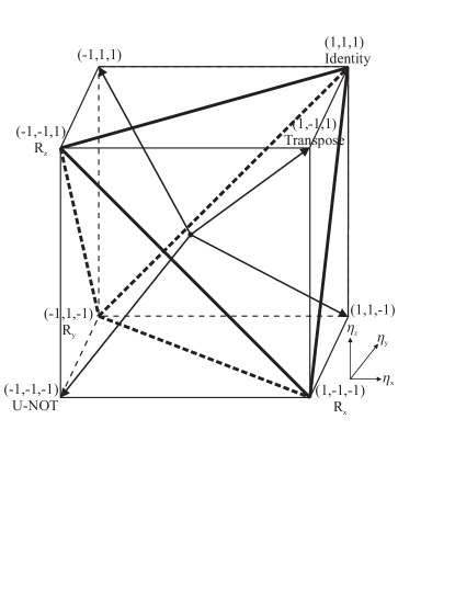
Figure 1: The completely positive unital, diagonal single-qubit maps as a subset of the positive ones. The axes $\eta_{\text{x}}$, $\eta_{\text{y}}$, and $\eta_{\text{z}}$ represent the diagonal “squeezing parameters”. Some special transformations, including the matrix transpose, the universal NOT, and the identity are also marked.

IV Simulating Quantum Channels

The set $\cal{D}$ is a regular tetrahedron with vertices I, $\text{R}_{\text{x}}$, $\text{R}_{\text{y}}$ and $\text{R}_{\text{z}}$, where I is the identity tranformation and the $\text{R}_{i}$s are rotations by $\pi$ about the x, y, z axes. Since the tetrahedron is a convex polyhedron, $\cal{D}$ is the convex hull of the points representing $I$ and the three rotations. Thus, every transformation corresponding to a point in $\cal{D}$ can be realised as a statistical mixture of those four extremal transformations. Such a transformation is sometimes referred to as a Pauli channel. Thus, we have

Property 2

$\vec{\eta}\in\cal{D}$ if and only if $\vec{\eta}$ corresponds to a Pauli channel.

Now, suppose $\mathcal{S}$ is a unital single-qubit quantum channel but A is not necessarily diagonal. A possesses a polar decomposition of the form $\text{A}=\text{s}\text{P}\text{R}$, where $\text{s}=\det(\text{A})$, $\text{P}=\left(\text{AA}^{\text{T}}\right)^{\frac{1}{2}}$, and R is a rotation Horn and Johnson (1985). Since sP is symmetric, there exists a rotation Q and a diagonal $\Delta$ such that $\text{sP}=\text{Q}\Delta\text{Q}^{\text{T}}$, giving

$$\text{A}=\text{Q}\Delta\text{Q}^{\text{T}}\text{R}.$$ (6)

Since both Q and $\text{Q}^{\text{T}}\text{R}$ are rotations, a general unital CP map on a single qubit can be decomposed into a rotation, followed by a diagonal transformation, followed by another rotation. Thus, we can construct a quantum computational network to simulate an arbitrary single-qubit unital quantum channel (Figure 2).

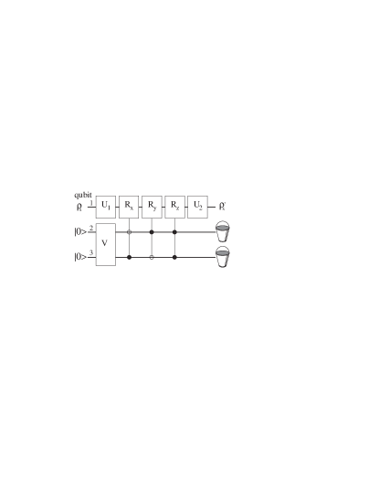
Figure 2: A quantum computational network for simulating a unital single-qubit quantum channel. Transformations $\text{U}_{1}$ and $\text{U}_{2}$ are qubit rotations while V prepares arbitrary superpositions of the states $\left|{00}\right\rangle,\left|{01}\right\rangle,\left|{10}\right\rangle,\left|{11}\right\rangle$ of the ancilla. After interacting with qubit 1, the ancilla is ignored. The controlled-controlled-$\text{R}_{i}$ gates perform the Pauli rotations depending on the component amplitudes of the ancilla.

V CP Map Dynamics

We can simulate a CP map dynamically by coupling the qubit to an ancilla with a time-independant Hamiltonian, evolving the whole system by the unitary, $\text{U}(\text{t})=\text{exp}\left(\frac{-i\text{Ht}}{\hbar}\right)$, and tracing over the ancilla. Thus, the final state of the qubit is a function of the interaction time. This gives us a class of maps on the single-qubit subsystem, parameterised by t, which depends on the coupling Hamiltonian. For unital maps, these classes corespond to paths in $\vec{\eta}$-space. It is again convenient to use a two-qubit ancilla. Consider the following Hamiltonians,

$$\text{H}_{\text{x}} = \sigma_{\text{x}}\otimes\left(\left|{\text{a}_{1}}\right\rangle\left\langle{\text{a}_{2}}\right|+\left|{\text{a}_{2}}\right\rangle\left\langle{\text{a}_{1}}\right|\right)$$ (7a)

$$\text{H}_{\text{y}} = \sigma_{\text{y}}\otimes\left(\left|{\text{a}_{1}}\right\rangle\left\langle{\text{a}_{3}}\right|+\left|{\text{a}_{3}}\right\rangle\left\langle{\text{a}_{1}}\right|\right)$$ (7b)

$$\text{H}_{\text{z}} = \sigma_{\text{z}}\otimes\left(\left|{\text{a}_{1}}\right\rangle\left\langle{\text{a}_{4}}\right|+\left|{\text{a}_{4}}\right\rangle\left\langle{\text{a}_{1}}\right|\right),$$ (7c)

where $\left\{\left|{\text{a}_{i}}\right\rangle\right\}$ are othornormal states of the ancilla, and the initial state of the system is $\rho_{0}\otimes\left|{\text{a}_{1}}\right\rangle\left\langle{\text{a}_{1}}\right|$. Each $\text{H}_{i}$ induces a set of CP maps in $\vec{\eta}$-space which form a straight line from I to the other corners of the tetrahedron, $\text{R}_{\text{x}}$, $\text{R}_{\text{y}}$ or $\text{R}_{\text{z}}$ respectively. If we combine these Hamiltonians together,

$$\text{H}_{\text{total}} = \alpha_{\text{x}}\text{H}_{\text{x}}+\alpha_{\text{y}}\text{H}_{\text{y}}+\alpha_{\text{z}}\text{H}_{\text{z}}$$

$$1 = \alpha_{\text{x}}^{2}+\alpha_{\text{y}}^{2}+\alpha_{\text{z}}^{2},$$ (8)

the map induced by $\text{H}_{\text{total}}$ is,

$$\vec{\eta}(\text{t})=(1,1,1)\cos^{2}\left(\frac{\text{t}}{\hbar}\right)+\left(2\alpha_{\text{x}}^{2}-1,2\alpha_{\text{y}}^{2}-1,2\alpha_{\text{z}}^{2}-1\right)\sin^{2}\left(\frac{\text{t}}{\hbar}\right)$$ (9)

This resulting set of maps is a line in $\vec{\eta}$-space connecting I to the convex combination of $\text{R}_{\text{x}}$, $\text{R}_{\text{y}}$ and $\text{R}_{\text{z}}$ weighted by the $\alpha_{i}^{2}$. For example, if $\alpha_{x}^{2}=\alpha_{y}^{2}=\alpha_{z}^{2}=\frac{1}{3}$, the resulting set of maps is a line from $(1,1,1)$ to $\left(-\frac{1}{3},-\frac{1}{3},-\frac{1}{3}\right)$. Thus, if we let the system evolve until $\text{t}=\frac{\pi\hbar}{2}$, the induced map is the best approximation to the Universal-NOT, as we shall see later. At $\text{t}=\frac{\pi\hbar}{3},\frac{2\pi\hbar}{3}$, the qubit is maximally mixed. Conversely, any unital CP map can be expressed as the result of some combination of $\text{H}_{\text{x}}$, $\text{H}_{\text{y}}$ and $\text{H}_{\text{z}}$ evolved for a particular time (Figures 3 and 4).

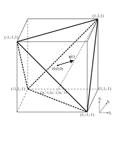
Figure 3: Dynamical generation of a CP map by suitable combination of coupling Hamiltonians and evolution times.

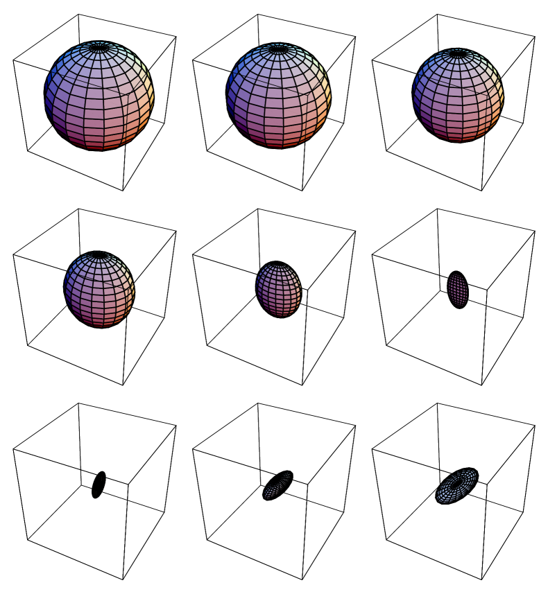
Figure 4: The Bloch sphere of the reduced density operator of the single qubit evolving in time with $\alpha_{\text{x}}^{2}=\frac{1}{2}$, $\alpha_{\text{y}}^{2}=\frac{1}{3}$ and $\alpha_{\text{z}}^{2}=\frac{1}{6}$.

VI Approximating Positive Maps

Now consider finding the CP map that best approximates a given positive map on a single qubit. We shall choose the metric on the space of positive maps induced by the inner product,

$$\langle\text{A},\text{B}\rangle=\text{Tr}(\text{A}^{\dagger}\text{B})$$ (10)

For the unital diagonal maps, this is simply the Euclidean distance in $\vec{\eta}$-space. Thus, finding the best unital, diagonal CP approximation to a given transformation is simply a matter of minimising the distance to the tetrahedron $\mathcal{D}$, in effect, dropping a perpendicular to the nearest face of $\mathcal{D}$ (Figure 5). This simplification has wide applicability because symmetry requirements on the approximating maps often necessitate the restriction to unital, diagonal maps anyway.

A simple example is the best approximation to the universal NOT gate on a single qubit Buzek et al. (1997). On the Bloch sphere, a perfect universal NOT corresponds to the transformation $\vec{\eta}=(-1,-1,-1)$. It is simply the map

$$\left|{\psi}\right\rangle\mapsto\beta^{*}\left|{0}\right\rangle-\alpha^{*}\left|{1}\right\rangle$$ (11)

that we observed was not physical in (1). Here, we need to drop a perpendicular to the plane

$$\eta_{\text{x}}+\eta_{\text{y}}+\eta_{\text{z}}=-1.$$ (12)

This yields the best approximation, $\vec{\eta}=(-\frac{1}{3},-\frac{1}{3},-\frac{1}{3})$ which was, of course, well-known. It is easy to check that this map can be constructed by selecting randomly from among the three options $\text{R}_{\text{x}}$, $\text{R}_{\text{y}}$, and $\text{R}_{\text{z}}$, each with probability one third.

The technique, however, applies equally well to less symmetrical positive maps not as amenable to the techniques used in Buzek et al. (1997). For example, the best approximation to the “pancake” map $\vec{\eta}=(1,1,0)$ is given by the map $\vec{\eta}=(\frac{2}{3},\frac{2}{3},\frac{1}{3})$. It is also easy to verify that the best approximation of the type $(\eta_{\text{x}},\eta_{\text{y}},0)$ is $\vec{\eta}=(\frac{1}{2},\frac{1}{2},0)$.

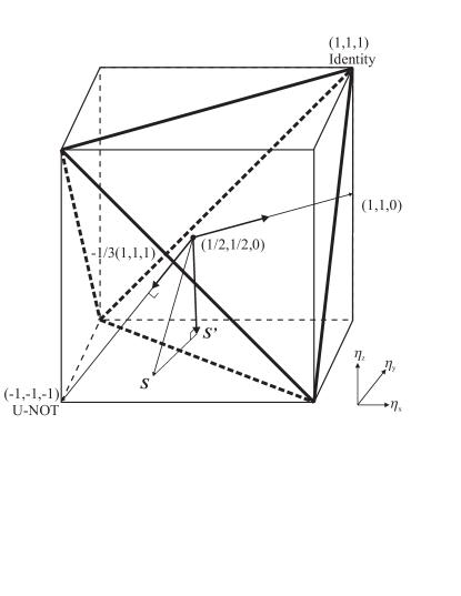
Figure 5: Both the universal NOT and a generic positive map are approximated by dropping perpendiculars to the closest face of $\cal{D}$.

VII Application to Quantum Eavesdropping

In the four-state Bennett and Brassard (1984) (resp. six-state Bruß (1998)) quantum key-distribution protocol, Alice sends one by one to Bob, qubits in one of four (six) states, $\{\left|{0}\right\rangle_{\theta},\left|{1}\right\rangle_{\theta}\}_{\theta}$ where $\theta\in\{\text{x},\text{z}\}$ ($\theta\in\{\text{x},\text{y},\text{z}\}$) is a choice of basis and $\left|{0}\right\rangle_{\text{z}}=\left|{0}\right\rangle$, $\left|{1}\right\rangle_{\text{z}}=\left|{1}\right\rangle$, $\left|{0}\right\rangle_{\text{x}}=(\left|{0}\right\rangle+\left|{1}\right\rangle)/2$, $\left|{1}\right\rangle_{\text{x}}=(\left|{0}\right\rangle-\left|{1}\right\rangle)/2$, $\left|{0}\right\rangle_{\text{y}}=(\left|{0}\right\rangle+i\left|{1}\right\rangle)/2$ and $\left|{1}\right\rangle_{\text{y}}=(\left|{0}\right\rangle-i\left|{1}\right\rangle)/2$. Bob measures each qubit in a random basis $\theta^{\prime}\in\{\text{x},\text{z}\}$ ($\theta^{\prime}\in\{\text{x},\text{y},\text{z}\}$) chosen independently of $\theta$. After the quantum transmission, Alice and Bob compare their bases publicly. For each qubit, if their bases correspond, Alice and Bob should share the same bit value, provided the qubits were not tampered with during the transmission. They estimate the error rate or the disturbance of the quantum channel by comparing a sample of these bits. The key distribution is validated if this disturbance is smaller than a certain specified threshold.

Many eavesdropping scenerios against quantum cryptographic protocols have been studied. In particular, in an incoherent attack, a possible spy, Eve, interacts each qubit, sent by Alice to Bob, with a probe. One can assume, without loss of generality, that the probe is in a pure state $\left|{\text{E}}\right\rangle$. The unitary operator that Eve uses to interact her probe with Alice’s qubits is identical in each case. In the basis $\theta\in\{\text{x},\text{z}\}$ (or $\theta\in\{\text{x},\text{y},\text{z}\}$)

$$\text{U}\left|{0}\right\rangle_{\theta}\left|{\text{E}}\right\rangle = \left|{\text{E}_{00}}\right\rangle_{\theta}\left|{0}\right\rangle_{\theta}+\left|{\text{E}_{01}}\right\rangle_{\theta}\left|{1}\right\rangle_{\theta}$$ (13)

$$\text{U}\left|{1}\right\rangle_{\theta}\left|{\text{E}}\right\rangle = \left|{\text{E}_{10}}\right\rangle_{\theta}\left|{0}\right\rangle_{\theta}+\left|{\text{E}_{11}}\right\rangle_{\theta}\left|{1}\right\rangle_{\theta},$$ (14)

where the $\left|{\text{E}_{ij}}\right\rangle_{\theta}$ are possibly not normalised nor orthogonal states for Eve’s probe. After transmission of qubits, Eve stores her probes until the public announcement of the bases and measures them accordingly. However, Eve is limited to measuring her probes individually. In a symmetric incoherent attack, the quantum channel described above is a Pauli channel $(\eta_{\text{x}},\eta_{\text{y}},\eta_{\text{z}})$ with $\eta_{\text{x}}=\eta_{\text{z}}=\eta$ for the four-state protocol and $\eta_{\text{x}}=\eta_{\text{y}}=\eta_{\text{z}}=\eta$ for the six-state protocol. This implies that, for any basis $\theta$,

$$\,{}_{\theta}\langle\text{E}_{01}|\text{E}_{01}\rangle_{\theta} = \,{}_{\theta}\langle\text{E}_{10}|\text{E}_{10}\rangle_{\theta}=\frac{1-\eta}{2}=\text{D}$$ (15)

$$\,{}_{\theta}\langle\text{E}_{00}|\text{E}_{00}\rangle_{\theta} = \,{}_{\theta}\langle\text{E}_{11}|\text{E}_{11}\rangle_{\theta}=\frac{1+\eta}{2}=\text{F}=1-\text{D}$$ (16)

$$\,{}_{\theta}\langle\text{E}_{00}|\text{E}_{11}\rangle_{\theta} = \,{}_{\theta}\langle\text{E}_{11}|\text{E}_{00}\rangle_{\theta}=\left\{\begin{array}[]{cl}(\eta+\eta_{\text{y}})/2&\text{4-state}\\ \eta&\text{6-state}\end{array}\right.$$ (19)

The quantity D, called disturbance, is the probability, given that they choose the same basis, Alice and Bob get a different bit. Similarly, the quantity F is called fidelity since it is the probability, given Alice and Bob choose the same basis, they get the same bit. Let $\text{p}_{\text{c}}$ be the probability that given Alice and Bob share the same basis and the same bit, Eve guesses correctly the value of this shared bit. When Alice and Bob share the same basis and the same bit, Eve has to guess whether her probe is in state $\frac{1}{\text{F}}\left|{\text{E}_{00}}\right\rangle_{\theta\,\theta}\left\langle{\text{E}_{00}}\right|$ or in the state $\frac{1}{\text{F}}\left|{\text{E}_{11}}\right\rangle_{\theta\,\theta}\left\langle{\text{E}_{11}}\right|$. If Eve uses the optimal measurement to guess this bit value,

$$\text{p}_{\text{c}}=\frac{1}{2}+\frac{1}{2}\sqrt{1-\frac{1}{\text{F}}|\,_{\theta}\langle\text{E}_{00}|\text{E}_{11}\rangle_{\theta}|^{2}}.$$ (20)

Eve’s objective is to maximise $\text{p}_{\text{c}}$ given an allowed disturbance level. In other words, given $\eta\geq\eta_{min}$ where $(1-\eta_{\text{min}})/2=\text{D}_{\text{max}}$ is the maximum allowed disturbance, Eve has to minimise $|\,_{\theta}\langle\text{E}_{00}|\text{E}_{11}\rangle_{\theta}|$. Referring to the tetrahedron representing $\mathcal{D}$, it is easy to see that such a minimum is reached for $\vec{\eta}=(\eta_{\text{min}},2\eta_{\text{min}}-1,\eta_{\text{min}})$ for the four-state protocol (Figure 6) and $\vec{\eta}=(\eta_{\text{min}},\eta_{\text{min}},\eta_{\text{min}})$ for the six-state protocol (Figure 7). This is precisely the results obtained by Cirac and Gisin in Cirac and Gisin (1997).

It should be noted that the same analysis can be applied to protocols involving distribution of EPR pairs between Alice and Bob Ekert (2000) and, in essence, the same results apply.

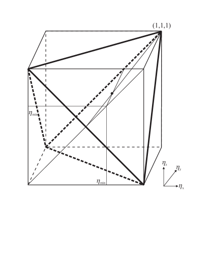
Figure 6: For the four-state protocol with $\eta_{\text{x}}=\eta_{\text{z}}=\eta\geq\eta_{\text{min}}$, Eve has to minimise $\eta_{\text{y}}$. When $\eta_{\text{min}}$ is positive, the minimum lies on the plane $\{(1,1,1),(-1,-1,1),(1,-1,1)\}$.

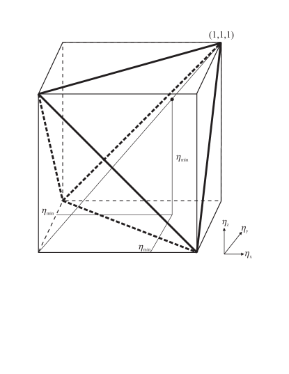
Figure 7: For the six-state protocol, with $\eta_{\text{x}}=\eta_{\text{y}}=\eta_{\text{z}}=\eta\geq\eta_{\text{min}}$, the minimum is reached for $\eta=\eta_{\text{min}}$.

VIII Strømer-Woronowicz Result

Horodecki’s proof Horodecki (1997) of Peres’ separability criterion Peres (1998) for 2 by 2 and 2 by 3 dimensional quantum systems relies crucially on an older result of Strømer and Woronowicz Woronowicz (1976) stating that any positive map $\mathcal{P}$ from a 2 dimensional quantum system to a 2 or 3 dimensional quantum system can be decomposed in the form

$$\mathcal{P}=\mathcal{CP}_{1}+\mathcal{CP}_{2}\circ\mathcal{T},$$ (21)

where $\mathcal{CP}_{1}$ and $\mathcal{CP}_{2}$ are completely positive maps and $\mathcal{T}$ is the transpose map. The geometry of $\cal{D}$ will again make the reason clear for the 2 by 2 dimensional, unital case.

The maps in (21) are not neccessarily trace preserving so it is convenient to consider an equivalent result,

$$\mathcal{P}=\text{p}\mathcal{CP}_{1}+(1-\text{p})\mathcal{CP}_{2}\circ\mathcal{T},$$ (22)

where $0\leq\text{p}\leq 1$ and $\mathcal{CP}_{1}$ and $\mathcal{CP}_{2}$ are now trace preserving. Thus, $\mathcal{P}$ can be expressed as the convex combination of $\mathcal{CP}_{1}$ and $\mathcal{CP}_{2}\circ\mathcal{T}$.

Furthermore, observe that $\mathcal{T}$ corresponds to the point $(1,-1,1)$ in Figure 1 and is equivalent to the points $(-1,-1,-1)$, $(-1,1,1)$ and $(1,1,-1)$ up to rotations of the tetrahedron. Since rotations correspond to unitary transformations, which are invertible CP maps, any of the above 3 transformations can be substituted for $\mathcal{T}$ in (21).

Now, given any point inside the cube of Figure 1 representing a positive map $\mathcal{P}$, it either lies within $\mathcal{D}$, or within one of the four pyramidal regions. If it lies within the tetrathedron, then the proof is trivial. If the map lies outside $\mathcal{D}$, the map is positive but not completely positive and we need to show that it can be decomposed into $\mathcal{CP}_{1}$ and $\mathcal{CP}_{2}\circ\mathcal{T}$, where $\mathcal{CP}_{1}$ and $\mathcal{CP}_{2}$ both lie within $\mathcal{D}$.

To simplify the argument, let us consider the corner region of the U-NOT map $(-1,-1,-1)$. By symmetry, the following argument can be applied to the other three corners regions. By constructing a line between the map $(-1,-1,-1)$ and the face of the tetrahedron whose vertices are $\text{R}_{\text{x}}$, $\text{R}_{\text{y}}$ and $\text{R}_{\text{z}}$, passing through the map $\mathcal{P}$, the proof is now apparent. Every $\mathcal{P}$ can be decomposed in this way as the non-CP pyramidal region is convex with extreme points, $(-1,-1,-1)$, $\text{R}_{\text{x}}$, $\text{R}_{\text{y}}$ and $\text{R}_{\text{z}}$. Figure 8 illustrates the situation.

Figure 8: The map $\mathcal{P}$ is decomposed into components $\mathcal{CP}_{1}$ and $\mathcal{CP}_{2}\circ\text{U-NOT}$ lying entirely within $\cal{D}$.

IX Conclusion

We have seen how the tetrahedral geometry of the set of unital, diagonal single-qubit channels can be used to motivate solutions to a number of problems in quantum information theory. The question of whether the techniques can be extended to non-unital maps or to higher dimensions remains open.

Appendix

The CP conditions (3) can be easily derived by ensuring that the trivial extension of a positive map to a maximally entangled state is positive. Let $\mathcal{S}:\mathcal{B}(C^{d})\mapsto\mathcal{B}(C^{d})$ be a linear operator and let $\left|{\Psi_{+}}\right\rangle=\text{N}^{-\frac{1}{2}}\sum_{i}\left|{i}\right\rangle\left|{i}\right\rangle$ be a maximally entangled state. Then

$$(\leavevmode\hbox{\small 1\kern-3.8pt\normalsize 1}\otimes\mathcal{S})\left|{\Psi_{+}}\right\rangle\left\langle{\Psi_{+}}\right|\geq 0,$$ (23)

iff $\mathcal{S}$ is CP. To see this, if $\mathcal{S}$ is not CP, $\exists\left|{\Phi}\right\rangle\in\mathcal{H}\otimes\mathcal{H}$ such that $(\leavevmode\hbox{\small 1\kern-3.8pt\normalsize 1}\otimes\mathcal{S})\left|{\Phi}\right\rangle\left\langle{\Phi}\right|\not\geq 0$. We can express,

$$\left|{\Phi}\right\rangle=(\mathcal{A}\otimes\leavevmode\hbox{\small 1\kern-3.8pt\normalsize 1})\left|{\Psi_{+}}\right\rangle,$$ (24)

where $\mathcal{A}$ is CP and its components are,

$$\left\langle{m}\right|\text{A}\left|{n}\right\rangle = \sqrt{\text{N}}a_{mn}$$

$$(\text{A}\otimes\leavevmode\hbox{\small 1\kern-3.8pt\normalsize 1})\left|{\Psi_{+}}\right\rangle = \sum_{m,n}a_{mn}\left|{m}\right\rangle\left|{n}\right\rangle$$

$$\rho \mapsto \text{A}\rho\text{A}^{\dagger}.$$ (25)

Thus, we have that,

$$(\leavevmode\hbox{\small 1\kern-3.8pt\normalsize 1}\otimes\mathcal{S})(\mathcal{A}\otimes\leavevmode\hbox{\small 1\kern-3.8pt\normalsize 1})\left|{\Psi_{+}}\right\rangle\left\langle{\Psi_{+}}\right| \not\geq 0$$

$$(\mathcal{A}\otimes\leavevmode\hbox{\small 1\kern-3.8pt\normalsize 1})(\leavevmode\hbox{\small 1\kern-3.8pt\normalsize 1}\otimes\mathcal{S})\left|{\Psi_{+}}\right\rangle\left\langle{\Psi_{+}}\right| \not\geq 0$$

$$\Rightarrow\quad(\leavevmode\hbox{\small 1\kern-3.8pt\normalsize 1}\otimes\mathcal{S})\left|{\Psi_{+}}\right\rangle\left\langle{\Psi_{+}}\right| \not\geq 0,$$ (26)

hence we only need look at the action of $\leavevmode\hbox{\small 1\kern-3.8pt\normalsize 1}\otimes\mathcal{S}$ on the maximally entangled state $\left|{\Psi_{+}}\right\rangle$ to ensure that $\mathcal{S}$ is CP.

References

- Fujiwara and Algoet (1999) A. Fujiwara and P. Algoet, Physical Review A59(5), 3290 (1999).
- Ruskai et al. (2001) M. B. Ruskai, S. Szarek, and E. Werner (2001), eprint LANL e-print quant-ph/0101003.
- Ruskai (1999) M. B. Ruskai, Minimal entropy of states emergy from noisy quantum channels (1999), eprint LANL e-print quant-ph/9911079.
- di Vincenzo and Terhal (1998) D. di Vincenzo and B. Terhal (1998), eprint LANL e-print quant-ph/9806095.
- Horn and Johnson (1985) R. Horn and C. Johnson, Topics in Matrix Analysis (Cambridge University Press, 1985).
- Buzek et al. (1997) V. Buzek, M. Hillery, and R. Werner, Optimal manipulations with qubits: Universal not gate (1997), eprint LANL e-print quant-ph/9711070.
- Bennett and Brassard (1984) C. Bennett and G. Brassard, eds., Proceedings of IEEE International Conference on Computers, Systems and Signal Processing (Banglore, India, 1984).
- Bruß (1998) D. Bruß, Phys. Rev. Lett. 81, 3018 (1998).
- Cirac and Gisin (1997) I. Cirac and N. Gisin, Phys. Lett. A 229, 1 (1997).
- Ekert (2000) A. Ekert, in Proceedings of the Conference in Commemoration of John Bell, “Quantum (Un)Speakables” (University of Vienna, 2000).
- Horodecki (1997) P. Horodecki, Phys. Lett. A 232, 333 (1997).
- Peres (1998) A. Peres, in Proceedings of Nobel Symposium 104: Modern Studies of Basic Quantum Concepts and Phenomena (1998), vol. 76.
- Woronowicz (1976) S. L. Woronowicz, Rep. Math. Phys. 10, 165 (1976).