Kerr cat states from the four-photon Jaynes-Cummings model
Abstract
We investigate the dynamics of a four-photon Jaynes-Cummings model for large photon number. It is shown that at certain times the cavity field is in a pure state which is a superposition of two Kerr states, analogous to the Schrödinger cat state (superposition of two coherent states) which occurs in the one and two photon cases.
1 Introduction
The Jaynes-Cummings model (JCM) is a standard and important model which describes the interaction of an atom and a single mode radiation field in a cavity [1, 2]. The importance of this model is due not only to its exact solvability, but also arises from some of its purely quantum effects, such as the periodic collapse and revival of the atomic number population, and the behaviour of the cavity field which becomes a Schrödinger cat state - a phase-correlated superposition of two coherent states - at certain times. The JCM model has been generalized in many different ways. One such is the multiphoton generalization [2] described by the following Hamiltonian ()
| (1.1) |
where is a positive integer, , and are atomic operators, is the coupling constant, and are the atomic transition frequency and cavity resonant mode frequency respectively. It is interesting that for both the one [3] and two [4, 5] photon cases, the cavity field is in a Schrödinger cat state at intervals corresponding to one half of the revival time. This arises from the fact that the Rabi frequency in both cases is proportional to (up to a constant) in the approximation of large photon number [3, 4, 5].
In this paper we shall address the dynamics and quantum characteristics of the 4-photon JCM in the large photon number approximation. Under this approximation the generalized Rabi frequency (Eq.(2.3)) depends on nonlinearly (up to ) and this nonlinearity causes Kerr nonlinearity in the cavity. We shall study the photon number distribution (Sec. 3) and the entropy of the cavity field (Sec.4) and the Q-function (Sec. 5). It is found that the cavity field is in a Kerr state or a macroscopic superposition of two Kerr states at certain times. We also study the atomic number inversion and find that it exhibits collapse and revival for short time intervals.
2 Large photon number approximation
We assume that at the initial time , the atom and field are decoupled and the atom is initially prepared in the excited state , while the field is in the coherent state
| (2.1) |
where is a complex number. For simplicity, we only consider the on-resonance interaction case as in [4]. Then the combined atom-field wave function at time is obtained as
| (2.2) |
where is the scaled time and is the generalized Rabi frequency [6] (in units of )
| (2.3) |
In the large photon number case, namely when the average photon number is large enough (, the Poisson distribution is mainly concentrated near and we have .
We now specialize to the case . To facilitate an analytical treatment, we write the generalized Rabi frequency as
| (2.4) |
For the large photon number case, is a small term and we can use the following Taylor expansion
| (2.5) |
Here we can only neglect the terms in which are much smaller than 1, namely, we must keep the terms to in (2.5). This is because is the argument of trigonometric functions in the wave function (2.2) and a small constant (for example ) can effect the physical quantity drastically. We therefore need to calculate the first three terms in (2.5). We then obtain the approximate generalized Rabi frequency
| (2.6) |
and . Here the constant terms (5 or 1) are much smaller than but cannot be neglected.
3 Photon number distribution
Taking the trace in the atom space, one finds for the reduced density operator of the cavity field
| (3.1) |
from which the photon number distribution (PND) is obtained as
| (3.2) | |||||
It is easy to see that the PND is a -periodic function of the scaled time . This means that at , we have , a Poisson distribution. At , we have , where we have used that fact that is always an odd integer. This means that the PND is also a Poisson distribution, but displaced by 4. However, the wave function (pure state) is not necessarily a coherent state; we shall see in the next section that the wave function is actually a Kerr state [7].
When , we have and therefore
| (3.3) |
Writing , we have
| (3.4) |
Then the PND is finally obtained as
| (3.5) |
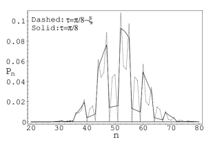
namely, the average of PND at and , as shown in Fig.1.
When , and the PND is obtained as
| (3.6) |
which is a strongly oscillating function; in other words, the photon number distribution exhibits strong oscillation. Writing , we can further write (3.6) as
| (3.7) |
So for any the photon number distribution is non-vanishing and, in that sense, the oscillation is not perfect. However, as can be seen from Fig.1, at the slightly earlier time , the photon number distribution exhibits perfect oscillation in that it becomes zero at and .
4 Entropy and pure states of the cavity field
The entropy of a quantum-mechanical system is a measure of how close the system is to a pure state and is defined by [8, 9]
where is the density operator of the quantum system and the Boltzmann constant is assumed to be unity. for a pure state and for a mixed state. In our model, the initial state is prepared in a pure state, so the whole atom-field system remains in a pure state at any time and its entropy is always zero. However, due to the entanglement of the atom and the cavity field at , both the atom and the field are generally in mixed states, although at certain times the field and the atomic subsystems are ‘almost’ in pure states.
Since the initial state is a pure state, the entropy of the cavity field equals the atomic entropy [9]. The entropy or , which is referred to as the entanglement of the total system in quantum information, is used to measure the amount of entanglement between the two subsystems. When , the system is disentangled or separable and both the field and atomic subsystems are in pure states.
It is more convenient to calculate the entropy of the 2-level atomic system. From Eq.(2.2) the atomic reduced density operator can be readily obtained as
| (4.8) |
where
| (4.9) |
The field and atomic entropy can be expressed as
| (4.10) |
where are the eigenvalues of the atomic reduced field density operator
| (4.11) |
Noting that is an odd integer for large photon number, it is easy to see that the entropy of the cavity field is a -periodic function of . We plot the entropy as a function of for and in Fig.2. We observe that the entropy is dynamically reduced to zero at and the cavity field can be periodically found in pure states. We also observe that the entropy falls quickly to minima near (see also Fig.3).
Those calculated features can be explained analytically. The periodicity of implies that for any positive integer . In this case the wave function (2.2) can be readily obtained as
| (4.12) |
namely, the cavity field is in the coherent state (up to a phase).
When , we have and thus the entropy . In this case the wave function of the system is
| (4.13) |
that is, the atom is in its ground state and the field is in a pure state, which is known as a Kerr state [7]
| (4.14) |
When the atom is detected in its ground state, the cavity field will be in the Kerr state.
When and , we have and , where we have used the following fact for large photon number
| (4.15) |
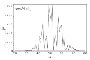
The entropy is then (The exact numerical result is 0.69314, see Fig.3). This means that the cavity field is in a mixed state. However, at a slightly earlier or later time , the entropy is dramatically reduced to a minimum, as can be seen in Fig.2 and Fig.3. For the specific choice
| (4.16) |
we obtain
| (4.17) |
where we have used the relation for large photon number . In this case we can see that the entropy is approximately zero. In fact, at , using (4.17) we obtain the following factorized state (writing )
| (4.18) | |||||
from which we see that the cavity field is a macroscopic superposition of two Kerr states
| (4.19) |
5 The Q-function and Population Inversion
The quasi-probability distribution Q-function is defined as [10]:
| (5.1) |
where is the reduced density operator of the cavity field given in Eq. (3.1) and is a coherent state. Inserting Eq. (3.1) into Eq. (5.1) we can easily obtain the Q-function of the cavity field
| (5.2) |
When and , the cavity field is in a coherent state and its Q-function is Poissonian, as can be seen from Fig. 5. At , the Q-function has two components. At , the Q-function has 8 components, and the field is in a mixed state (its entropy is 0.6888). So the interference between components results in imperfect oscillation of the PND.
When the Q-function is composed of 4 well-separated components, the entropy reaches its maximum and the field is in a mixed state. In a short time , the field is nearly pure and the Q-function separates into 8 components, the interference between which resulting in strong oscillation of the PND, as can be seen from Fig.(4). However, at and the cavity field is less pure and the Q-function has less well-separated components, and the oscillation of the PND is less marked (see Fig.4).
Finally, we briefly describe the atomic population inversion (API), given by
| (5.3) |
In the one or two photon cases this exhibits the usual periodic collapse and revival phenomenon. The 4-photon system also shows this behaviour. In Fig.6 we give a plot of the API for , from which one can see that the API for the 4-photon system also exhibits periodic collapse and revival. However, due to the nonlinearity of the system, this effect does not last as long as in the one or two photon cases.
6 Conclusions
In this paper we studied the four-photon JC model and its dynamical behaviour. In the large photon number approximation, the Rabi frequency depends quadratically on and this leads to nonlinear effects in the cavity.
By examining the entropy of the field or atom we found that the system is approximately disentangled at certain times. In this case both the atom and cavity field are in a pure state and those pure states are explicitly given. It is interesting that the cavity field exists in both a nonlinear Kerr state and a macroscopic superposition of Kerr states, analogous to the coherent state and the Schrödinger cat states in the one or two photon JC model. One may refer to this analogous Kerr superposition as a Kerr cat state.
We analysed the PND in the large photon number approximation. At certain times the PND exhibits strong oscillation. From the Q-function we know that the cavity field at those times has eight components; it is the interference between those components which causes the strong oscillation of the PND. Note that these oscillations depend more sensitively on the interaction time than in the one or two photon cases due to the quadratic dependence of the generalized Rabi frequency on photon number in the present work.
We also considered atomic number inversion and found that the phenomenon of periodic collapse and revival occurs; it is however a short-lived phenomenon due to the effects of nonlinearity.
Experimental implementation of the theoretical idea herein proposed would possibly depend on the use of a trapped neutral atom or ion in a high-Q cavity, or an atomic beam in transit through the cavity [11]. In any realistic scheme off-resonant effects must be taken into account, and for this reason the atomic species used must provide a good approximation to a two-level system.
Acknowledgements
We are grateful to Dr. Andrew Greentree for useful discussion and comment, especially with regard to the possible experimental realisation of the scheme proposed here. H. Fu is supported in part by the National Natural Science Foundation of China. A. I. S. thanks the Laboratoire de Physique Théorique des Liquides, Paris University VI, for hospitality.
References
- [1] Jaynes, E. T., and Cummings,F. W., 1963, Proc. IEEE, 51, 89.
- [2] Shore, B. W., and Knight, P. L., 1993, J. Mod. Opt. 40, 1195.
- [3] Gea-Banacloche, J., Phys. Rev. Lett. 65 3385.
- [4] Bužek, V., and Hladký, B., 1993, J. Mod. Opt. 40, 1309.
- [5] Fu, H. , Feng, Y., and Solomon, A. I., 2000, J. Phys. A., 33, 2231.
- [6] Normally the Rabi frequency is defined as . Here, for convenience, we include in the definition of the scaled time .
-
[7]
Kitagawa, M., and Yamamoto, Y., 1986,
Phys. Rev. A,
34, 3974;
Wilson-Gordon, A. D., Buzek, V., and Knight, P. L., 1991, Phys. Rev. A, 44, 7647. - [8] Wehrl, A., 1978, Rev. Mod. Phys., 50, 221.
- [9] Barnett S. M., and Phoenix, S. J. D., 1989, Phys. Rev. A, 40, 2042.
- [10] Hillery, M., O’Connel, R. F., Scully, M. O., and Wigner, E. P., 1984, Phys. Rep., 106 , 121.
- [11] Hood, C.J., Chapman, M. S., Lynn, T. W., and Kimble, H. J., 1998, Phys. Rev. Lett., 80, 4157; Munstermann P., Fischer, T., Maunz, P., Pinkse, P. W. H., and Rempe, G., 1999, Opt. Commun., 159, 63; 1999, Phys. Rev. Lett., 82, 3791.