Typical entanglement in multi-qubit systems

Abstract

Quantum entanglement and its paradoxical properties hold the key to an information processing revolution. Much attention has focused recently on the challenging problem of characterizing entanglement. Entanglement for a two qubit system is reasonably well understood, however, the nature and properties of multiple qubit systems are largely unexplored. Motivated by the importance of such systems in quantum computing, we show that typical pure states of $N$ qubits are highly entangled but have decreasing amounts of pairwise entanglement (measured using the Wootter’s concurrence formula) as $N$ increases. Above six qubits very few states have any pairwise entanglement, and generally, for a typical pure state of $N$ qubits there is a sharp cut-off where its subsystems of size $m$ become PPT (positive partial transpose i.e., separable or only bound entangled) around $N\gtrsim 2m+3$, based on numerical analysis up to $N=13$.

Quantum entanglement is a key prediction of quantum mechanics and is generally thought to be one of the crucial resources required in quantum information processing. Known quantum information applications include quantum computation divincenzo95a ; vedral98b , quantum communication schumacher96a , quantum cryptography ekert91a ; jennewein00a ; naik00a ; tittel00a , and quantum teleportation bennett93a ; bouwmeester97a ; boschi98a . The properties of entangled states potentially used in these applications are still poorly understood. General two qubit entangled states have been well characterized, and a number of analytical measures of entanglement are known wootters97a ; zyczkowski98a . However, for $N$ qubit systems (with $N>2$), few such measures can be calculated even for pure states. Despite these difficulties, arrays of qubits have been the focus of recent attention wootters00a ; oconnor00a ; koashi00a ; gunlycke01a , e.g., Raussendorf and Briegel raussendorf01a propose an array of highly entangled qubits for quantum computation.

In this letter we consider the average, or typical properties of $N$ qubit pure states. A subsystem of an entangled pure state is in general a mixed state, thus we also consider the entanglement of mixed states derived from these pure states. Currently, a variety of measures are known for quantifying the degree of entanglement, including the entanglement of distillation bennett96b , the relative entropy of entanglement vedral97b , the entanglement of formation wootters97a ; bennett96b and the negativity zyczkowski98a . Using $|0\rangle$ and $|1\rangle$ for the two eigenstates of a spin$-\frac{1}{2}$ system or equivalent that encodes a qubit, and $|00\rangle$ as a shorthand for $|0\rangle_{A}|0\rangle_{B}$, a state of two qubits $A$ and $B$, the four Bell states $(|00\rangle\pm|11\rangle)/\sqrt{2}$ and $(|01\rangle\pm|10\rangle)/\sqrt{2}$ have the maximum possible entanglement. Most entanglement measures assign a value of 1 to a Bell state, and 0 to all separable states.

For our purposes, it is convenient to use the tangle $\tau$ (squared concurrence) as our entanglement measure when considering two or three qubits. The tangle is an entanglement monotone from which the entanglement of formation can be calculated wootters97a ; coffman99a . For a pure state of two qubits, $\tau=4\text{det}|\rho_{A}|$, where $\rho_{A}$ is the reduced density matrix obtained when qubit $B$ has been traced over (or vice versa permuting $A$ and $B$). For a mixed state $\rho$ of two qubits, the concurrence $C=\tau^{1/2}$ is given wootters97a by

$$C=\text{max}(\lambda_{1}-\lambda_{2}-\lambda_{3}-\lambda_{4},0),$$ (1)

where the $\lambda_{i}$ are the square roots of the eigenvalues of $\rho\tilde{\rho}=\rho\;\sigma_{y}^{A}\!\otimes\!\sigma_{y}^{B}\rho^{*}\sigma_{y}^{A}\!\otimes\!\sigma_{y}^{B}$, and $\rho^{*}$ denotes the complex conjugation of $\rho$ in the computational basis $\{|00\rangle,|01\rangle,|10\rangle,|11\rangle\}$. The entanglement of formation $E_{f}=h(\frac{1}{2}+\frac{1}{2}\sqrt{1-C^{2}})$, where $h(x)$ is the binary entropy function, $h(x)=-x\log_{2}(x)-(1-x)\log_{2}(1-x)$.

A general pure state of two qubits can be written nemoto00a

$$|\Psi_{2}\rangle = e^{i\chi_{0}}\cos\theta_{0}|00\rangle$$ (2)

$$+ e^{i\chi_{1}}\sin\theta_{0}\cos\theta_{1}|01\rangle$$

$$+ e^{i\chi_{2}}\sin\theta_{0}\sin\theta_{1}\cos\theta_{2}|10\rangle$$

$$+ e^{i\chi_{3}}\sin\theta_{0}\sin\theta_{1}\sin\theta_{2}|11\rangle,$$

where $\chi_{j}$, $\theta_{j}$ are chosen uniformly according to

$$(2\pi)^{-4}\mathrm{d}(\sin\theta_{0})^{6}\mathrm{d}(\sin\theta_{1})^{4}\mathrm{d}(\sin\theta_{2})^{2}\mathrm{d}\chi_{0}\mathrm{d}\chi_{1}\mathrm{d}\chi_{2}\mathrm{d}\chi_{3},$$ (3)

the Haar measure, with $0\leq\chi_{i}<2\pi$ and $0\leq\theta_{i}<\pi/2$. (We include an extra overall random phase, $e^{i\chi_{0}}$, to maintain consistency with SU($n$).)

Calculating $\tau=4\text{det}|\rho_{A}|$ using Eq. (2) and integrating over the Haar measure, Eq. (3), gives $\langle\tau\rangle=2/5$. A randomly selected pure state of two qubits might thus be expected to have 0.4 tangle units of entanglement, and we have already noted that states exist with the maximum ($=1$) and minimum ($=0$) amounts of entanglement. More informative is the distribution, the density of states (over the Haar measure) with a given value of the tangle. Calculated numerically by sampling 30 million random pure states, this distribution is shown in Fig. 1.

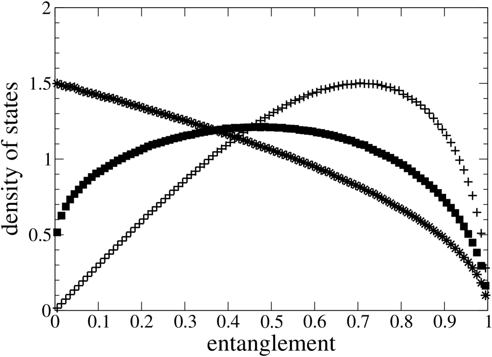
Figure 1: Distribution of the tangle ($\ast$), concurrence ($+$) and entanglement of formation ( ) for two qubit pure states sampled uniformly over the Haar measure.

In tangle units, the distribution is broad, with many states having little or no entanglement compared to only a few with high or maximal entanglement.

However, it must be emphasized that the shape of the distribution is heavily dependent on the choice of entanglement measure. Compare in Fig. 1 the distributions of the concurrence $C=\tau^{1/2}$ and the entanglement of formation (first shown in zyczkowski99a ). The corresponding average values (calculated numerically and in agreement with zyczkowski99a ) are $\langle C\rangle=0.5890\pm 0.0002$ and $\langle E_{f}\rangle=0.4808\pm 0.0002$. Given the plethora of entanglement measures in current use, it is important to only compare like with like. Also, it is interesting to note that, though close, none of these average entanglement values are exactly equal to 1/2, which would be the naïve guess.

For three qubits, it is possible to define the 3-tangle $\tau_{3}$ for a pure state coffman99a , giving a measure of the purely three-way entanglement in the system. A value for the tangle between each of the three possible pairs of qubits can also be calculated, $\tau_{AB}$, $\tau_{AC}$ and $\tau_{BC}$, using Eq. (1). These satisfy,

$$\tau_{3}=\tau_{A}-\tau_{AB}-\tau_{AC}$$ (4)

where $\tau_{A}=4\text{det}|\rho_{A}|$ as before, except now both qubits B and C have been traced out to leave the partial density matrix $\rho_{A}$. Equation (4) holds for any permutation of $A$, $B$ and $C$. For the GHZ state $(|000\rangle+|111\rangle)/\sqrt{2}$, which has the maximum possible 3-tangle, $\tau_{3}=1$ and $\tau_{AB}=0$, while for the W state $(|001\rangle+|010\rangle+|100\rangle)/\sqrt{3}$, $\tau_{3}=0$ and $\tau_{AB}=4/9$ for each pair, the maximum possible amount of pairwise tangle in a three qubit state koashi00a .

As for two qubits, the average values for $\tau_{3}$ and $\tau_{AB}$ can be calculated. After analytically evaluating somewhat lengthy integrals, they are found to be $\langle\tau_{3}\rangle=1/3$ and $\langle\tau_{AB}\rangle=1/6$. Since $\tau_{3}$ and $\tau_{AB}$ satisfy Eq. (4), one can consider the quantity $\langle\tau_{3}+\tau_{AB}+\tau_{AC}+\tau_{BC}\rangle=5/6$, the average total entanglement (in tangle units) in a random pure state of three qubits. This gives an average entanglement of $5/18\simeq 0.27$ per qubit for three qubits, compared with 1/5 per qubit for two qubits. A GHZ state has a tangle of 1/3 per qubit and a W state 4/9. O’Connor and Wootters wootters00a ; oconnor00a considered rings and chains of $N$ qubits in a translationally invariant state and determined the maximum possible nearest neigbour entanglement to be at least $C=0.434467$ or $\tau=0.18876157$ per qubit.

The distributions for $\tau_{3}$ and $\tau_{AB}$, Fig. 2 (inset), were calculated numerically by samping a million pure three qubit states drawn randomly over the Haar measure, the generalization of Eq. (3).

Figure 2: Distribution of the 2-tangle for two ($\ast$), three (filled $\triangle$) and four ( ) qubit pure states; inset: distribution of the 3-tangle ($\triangle$) and pairwise tangle (filled $\triangle$) for three qubit pure states, all sampled uniformly over the Haar measure.

The 2-tangle is now much more concentrated near zero than for two qubits, while the 3-tangle is broadly peaked around the average value.

These values for pairwise and three-way tangles would be more useful if it was possible to continue in the same manner for four and more qubits. Currently, there is no known analytical expression for the 3-tangle of a mixed state of three qubits, nor is it known whether expressions equivalent to Eq. (4) can be found beyond three qubits. However, we can at least continue to evaluate pairwise entanglement for larger pure states. For four qubits the average pairwise entanglement evaluated numerically from a million randomly sampled four qubit pure states is $0.03138\pm 0.00006$ tangle units per pair. Despite the low value for pairwise entanglement, a typical four qubit pure state is still highly entangled overall kempe01a , as can be shown by considering the entropy of its subsystems. For a pure state of N qubits, the entropy $S_{N}=0$. If the system is split into two pieces, of $k$ qubits and $(N-k)$ qubits, then each subsystem has the same entropy, $S_{k}=S_{(N-k)}=\sum_{i}\lambda_{i}\log_{2}\lambda_{i}$, where the $\lambda_{i}$ are the eigenvalues of the reduced density matrix $\rho_{k}$ obtained by tracing out the other $(N-k)$ qubits (or vice versa). The entropy $S_{k}$ measures how entangled the two subsystems are with each other. For four qubit pure states, $\langle S_{1}\rangle=\langle S_{3}\rangle=0.8661\dots$ and $\langle S_{2}\rangle=0.6653\dots$ normalised per qubit such that $0\leq S_{k}\leq 1$.

The four qubit pairwise distribution, shown in Fig. 2, is now strongly peaked around zero entanglement. A closer look at the numerical data reveals a new feature not present in the distributions for two or three qubit pure states: there is now a significant fraction of the pairs (24%) with zero entanglement, causing the outlying point at 67 for the bin that includes zero. This is not just zero to numerical accuracy. The formula for the concurrence of a pair of qubits in a mixed state $\rho$ is given by Eq. (1). Clearly, if the values of the $\lambda_{i}$ are such that the maximum is zero by a significant margin, then the result is effectively exact. This trend continues for random pure states of five and six qubits, with (evaluated numerically over samples of 100,000) 80% and 99% respectively of pairs having zero entanglement in such states selected randomly over the Haar measure. This is the probably $P_{2}$ of finding a chosen pair has zero entanglement. The probability $P_{s}$ that the state as a whole has zero pairwise entanglement in all possible pairs is smaller, but also fast approaching $100\%$; by $N=7$ numerical sampling gives $P_{s}>99.9\%$. So we have a picture of typical pure states having less and less pairwise entanglement as the number of qubits increases, with the measure of states with some pairwise entanglement becoming essentially zero beyond 7 qubits. In other words, the fall off is not gradual, but occurs sharply between $3<N\lesssim 7$.

This immediately begs the question, what happens to the entanglement in subsets of three or more qubits as N increases? While it isn’t known how to calculate the 3-tangle for mixed states of three qubits, there is another measure of entanglement that can be used to answer this question. The partial transpose of a density matrix expressed in the standard basis is obtained by interchanging terms with a selected qubit in the opposite state peres96a . Such a matrix, denoted $\rho^{T}$, can have negative eigenvalues if the original density matrix ${\rho}$ is entangled. If $\rho^{T}$ has only positive eigenvalues for any combination of transposed qubits (up to half the total in $\rho$), then $\rho$ is said to be PPT (positive partial transpose), and in most cases, $\rho$ is separable. The exceptions have bound entanglement horodecki97a ; horodecky98a , which only occurs in systems with Hilbert space larger than $2\otimes 2$. Bound entangled states are known to be relatively rare zyczkowski99a , of finite measure but smaller than the measure of separable states, which decreases exponentially in the number of qubits.

Figure 3: Average negativity for subsets of $m$ qubits selected from random pure states sampled uniformly over the Haar measure. The symbol gives $m$. For subsets of two qubits, the tangle ($\ast$) and concurrence($+$) are also shown.

A PPT test is sufficient to show that a three qubit subset has no free entanglement, but there is also a quantitative measure of entanglement that can be derived from $\rho^{T}$, the negativity. Following Życzkowski zyczkowski98a we define the negativity as twice the absolute value of the sum of the negative eigenvalues of $\rho^{T}$; Vidal and Werner vidal01a recently proved it is an entanglement monotone. Figure 3 shows how the average values compare with the tangle and concurrence, two curves are shown for subsets of four and five qubits because there are different values for transposing one qubit, or two qubits at once. A log-linear plot has been used to show that all the entanglement measures fall faster than exponentially as the number of qubits in the pure state increases.

Note, however, that the negativity does not satisfy any convenient quantitative relation like Eq. (4) for the tangle. It is thus not possible to identify finite amounts of three-way entanglement unless you also know that there is zero pairwise entanglement in the pure state. Conversely, if the negativity of all subsets of three qubits is zero, there is still the possibility of bound entanglement. Nonetheless, since bound entanglement is a relatively rare phenomenon, if we are willing to neglect it in order to obtain the shape of the larger picture over all pure states, we can use the negativity to identify states that have approximately zero entanglement in subsets of three, four and five qubits, Fig. 4.

Figure 4: Percentage of subsets of $m$ qubits with no (free) entanglement in random pure states sampled uniformly over the Haar measure, where $m$ is the symbol.

In each case, it drops sharply to zero between $N\simeq 2m$ and $N=2m+3$, based on numerical analysis of random pure states sampled uniformly over the Haar measure for $N\leq 13$ and $m\leq 6$.

This result can be explained at least qualitatively as follows. Page page93a conjectured (later proved foong94a ; sen96a ) that the average entropy of such a subsystem is (in the notation of this paper)

$$\langle S_{k}\rangle\,\ln(2) = \sum_{j=2^{N-k}+1}^{2^{N}}\frac{1}{j}\;-\frac{2^{k}-1}{2^{N-k+1}}$$ (5)

$$\simeq k\ln(2)-\frac{1}{2^{N-2k+1}}$$

where the approximate version is valid for $1\ll k\leq N/2$. These average entropies can also be calculated numerically in the same manner as we calculated the tangle and concurrence, by sampling random pure states. Comparison of these values with the theoretical formula provides a useful test of the accuracy of the numerical method, and agreement was generally better than 3 significant digits, even for relatively small sample sizes. A useful way of presenting $\langle S_{k}\rangle$ is shown in Fig. 5, where it is plotted per qubit for both the larger and smaller of the two subsystems.

Figure 5: Average entropy of subsystems plotted per qubit for random pure states sampled uniformly over the Haar measure. Symbols give subsystem size, $k$ and $(N-k)$. For $N=2$, the average entropy corresponds to $\langle E_{f}\rangle$ for two qubits, as shown.

Equation (5) implies that the entropy of the smaller subsystem is nearly maximal, which in turn implies that the subsystem is nearly maximally mixed, i.e. not entangled. In Fig. 5 this is shown by the lines for the smaller subsystem asymptoting to 1 as the difference between $k$ and $N$ becomes larger. There is a set of unentangled states of finite measure zyczkowski99a surrounding the maximally mixed state ($\rho=\bm{1}$). As $N$ increases and the smaller subsystem becomes more mixed, it enters this unentangled region for finite $N$, thus explaining the rapid transition to zero entanglement shown in Fig. 4.

In conclusion, we have shown that in randomly chosen pure states of $N$ qubits, there is a cut-off, $m$, below which subsets of qubits taken from the pure state by partial tracing over the remainder can be expected to be PPT (i.e. no free entanglement). For $N\leq 13$, the limited range accessible to our numerical studies, $m\gtrsim(N-3)/2$. There are already experimental situations (such as ion traps) with more than six distinguishable quantum particles in which such entangled states might be generated. Only looking for pairwise entanglement in such systems may give misleading results.

- (1) D. P. DiVincenzo, Science 270, 255 (1995).
- (2) V. Vedral and M. B. Plenio, Prog. Quant. Electron. 22, 1 (1998).
- (3) B. Schumacher, Phys. Rev. A 54, 2614 (1996).
- (4) W. Tittel, J. Brendel, H. Zbinden, and N. Gisin, Phys. Rev. Lett. 84, 4737 (2000).
- (5) T. Jennewein, C. Simon, G. Weihs, H. Weinfurter, and A. Zeilinger, Phys. Rev. Lett. 84, 4729 (2000).
- (6) D. S. Naik, C. G. Peterson, A. G. White, A. J. Berglund, and P. G. Kwiat, Phys. Rev. Lett. 84, 4733 (2000).
- (7) A. K. Ekert, Phys. Rev. Lett. 67, 661 (1991).
- (8) D. Boschi, S. Branca, F. De Martini, L. Hardy, and S. Popescu, Phys. Rev. Lett. 80, 1121 (1998).
- (9) C. H. Bennett, G. Brassard, C. Crépeau, R. Jozsa, A. Peres, and W. K. Wootters, Phys. Rev. Lett. 70, 1895 (1993).
- (10) D. Bouwmeester, J. W. Pan, K. Mattle, M. Eibl, H. Weinfurter, and A. Zeilinger, Nature 390, 575 (1997).
- (11) W. K. Wootters, Phys. Rev. Lett. 80, 2245 (1998), eprint quant-ph/9709029.
- (12) K. Życzkowski, P. Horodecki, A. Sanpera, and M. Lewenstein, Phys. Rev. A 58, 883 (1998), eprint quant-ph/9804024.
- (13) W. K. Wootters, Entangled chains (2000), eprint quant-ph/0001114.
- (14) K. M. O’Connor and W. K. Wootters, Phys. Rev. A 63, 052302 (2001), eprint quant-ph/0009041.
- (15) M. Koashi, V. Buz̃ek, and N. Imoto, Phys. Rev. A 62, 050302(R) (2000), eprint quant-ph/0007086.
- (16) D. Gunlycke, V. M. Kendon, V. Vedral, and S. Bose, Phys. Rev. A 64, 042302 (2001), eprint quant-ph/0102137.
- (17) R. Raussendorf and H. J. Briegel, Phys. Rev. Lett. 86, 5188 (2001).
- (18) C. H. Bennett, D. P. DiVincenzo, J. A. Smolin, and W. K. Wootters, Phys. Rev. A 54, 3824 (1996).
- (19) V. Vedral, M. B. Plenio, K. Jacobs, and P. L. Knight, Phys.Rev. A 56, 4452 (1997), eprint quant-ph/9703025.
- (20) V. Coffman, J. Kundu, and W. K. Wootters, Phys. Rev. A 61, 052306 (2000), eprint quant-ph/9907047.
- (21) K. Nemoto, J. Phys. A: Math. Gen. 33, 3493 (2000), eprint quant-ph/0004087.
- (22) K. Życzkowski, Phys. Rev. A 60, 3496 (1999), eprint quant-ph/9902050.
- (23) M. A. Nielsen and J. Kempe, Phys. Rev. Lett. 86(22), 5184 (2001), eprint quant-ph/0011117.
- (24) A. Peres, Phys. Rev. Lett. 77, 1413 (1996), eprint quant-ph/9604005.
- (25) P. Horodecki, Phys. Lett. A 232, 333 (1997), eprint quant-ph/9703004.
- (26) M. Horodecki, P. Horodecki, and R. Horodecki, Phys. Rev. Lett. 80, 5239 (1998), eprint quant-ph/9801069.
- (27) G. Vidal and R. F. Werner, A computable measure of entanglement (2001), eprint quant-ph/0102117.
- (28) D. N. Page, Phys. Rev. Lett 71, 1291 (1993), eprint gr-qc/9305007.
- (29) S. K. Foong and S. Kanno, Phys. Rev. Lett. 72, 1148 (1994).
- (30) S. Sen, Phys. Rev. Lett. 77, 1 (1996), eprint hep-th/9601132.