Entanglement in squeezed two-level atom

Abstract. In the previous paper, we adopted the method using quantum mutual entropy to measure the degree of entanglement in the time development of the Jaynes-Cummings model [1]. In this paper, we formulate the entanglement in the time development of the Jaynes-Cummings model with squeezed states, and then show that the entanglement can be controlled by means of squeezing.

Key words: entanglement, mutual entropy, Jaynes-Cummings model, squeezed state, quantum information theory

1 Introduction

Recently, it has been known that a quantum entangled state plays an important role in the field of quantum information theory such as quantum teleportation and quantum computation. The research on quantifying entangled states has been done by several measures[2, 3].

If we want to quantify entangled states, we should know whether they are pure states or mixed states. That is, if the entangled states are pure states, then it is well known that it is sufficient to use von Neumann entropy[4] for the reduced states[2, 3]. Because, for pure states, it has a unique measure. However, for mixed states, it does not have a unique measure. Therefore we need a proper measure of entanglement for mixed state. The degree of entanglement for mixed states has been studied by some entropic measures such as entanglement of formation[2] and quantum relative entropy[3] and so on. V.Vedral et al. defined the degree of the entangled states $\sigma$ as a minimum distance between all disentangled states $\rho\in{\cal D}$ such that $E\left(\sigma\right)\equiv{\min_{{}_{\rho\in{\cal D}}}}D\left(\sigma||\rho\right)$ where $D$ is any measure of distance between the two states $\sigma$ and $\rho$. For an example, we can choose quantum relative entropy as $D$. Then,

$$E\left(\sigma\right)={\min_{\rho\in{\cal D}}}S\left(\sigma|\rho\right),$$ (1)

where $S\left(\sigma|\rho\right)\equiv tr\sigma\left(\log\sigma-\log\rho\right)$ is quantum relative entropy[5, 6]. Since this measure has to take a minimum over all disentangled states, it is difficult to calculate analytically for the actual model such as the Jaynes-Cummings model so that we use the degree of entanglement due to mutual entropy[7], we call it DEM in the sequel, defined below. Moreover, there has been no fixed-definition of entanglement measure, though some measures have been defined other than the above measure defined in (1). So we can use the convenient measure which ever we want case-by-case.

Let $\sigma$ be a state in ${\mathfrak{S}}_{1}\otimes{\mathfrak{S}}_{2}$ and $\rho_{k}$ are the marginal states in ${\mathfrak{S}}_{k}$ (i.e., $tr_{j}\sigma=\rho_{k}\left(k\neq j\right)$ ). Then our degree of entanglement due to mutual entropy (DEM) is defined by:

$$I_{\sigma}\left(\rho_{1},\rho_{2}\right)\equiv tr\sigma\left(\log\sigma-\log\rho_{1}\otimes\rho_{2}\right).$$

Note that the tensor product state $\rho_{1}\otimes\rho_{2}$ is one of the disentangled states. This DEM represents the difference between the entangled states and disentangled states. This quantity is also applied to classify entanglement in [8]. If we treat only entangled pure states, it is sufficient to apply von Neumann entropy for the reduced states $\rho_{k}\equiv tr_{j}\sigma\in{\mathfrak{S}}_{k},(k\neq j)$. Because we suppose that $\sigma\in{\mathfrak{S}}_{1}\otimes{\mathfrak{S}}_{2}$ are entangled pure states, then its von Neumann entropy is equal to $0$ ($S\left(\sigma\right)=0$). Moreover, according to the following triangle inequality of Araki and Lieb[9]:

$$|S\left(\rho_{1}\right)-S\left(\rho_{2}\right)|\leq S\left(\sigma\right)\leq S\left(\rho_{1}\right)+S\left(\rho_{2}\right)$$

we have $S\left(\rho_{1}\right)=S\left(\rho_{2}\right)$. Thus we have

$$I_{\sigma}\left(\rho_{1},\rho_{2}\right) = tr\sigma\left(\log\sigma-\log\rho_{1}\otimes\rho_{2}\right)$$

$$= S\left(\rho_{1}\right)+S\left(\rho_{2}\right)-S\left(\sigma\right)$$

$$= 2S\left(\rho_{1}\right)$$

Therefore, for entangled pure states, the DEM becomes twice of the entropy of the induced marginal states. That is, if we want to know the degree of the entangled pure states, it is sufficient to use the reduced von Neumann entropy. However, in general the reduced von Neumann entropies for entangled mixed states are not always unique, namely, they depend on the way to take the partial trace, therefore we need the unique measure for the entangled mixed states. Thus in this paper we apply the DEM not the reduced von Neumann entropy in order to measure the degree of entanglement for the entangled mixed states, because the DEM can measure the degree of entanglement directly without taking partial trace. From (1), we also find that the entanglement degree in pure states is bigger than that in mixed states. In this short paper, we will formulate the entanglement degree in the Jaynes-Cummings model with squeezed states using DEM and then, try to control it by means of the squeezing parameter $r$.

2 Atomic system

The quantum electrodynamical interaction of a single two-level atom with a single mode of an electromagnetic field is described by the well known Jaynes-Cummings model(JCM)[10]. The JCM is the simplest nontrivial model of two interacting fully quantum systems and has an exact solution. It also brings us some interesting phenomena such as collapses and revivals. It has been investigated in detail by many researchers from various points of view. For details, the reader may refer to the excellent reviews [11, 12]. The JCM is not only an important problem itself but also gives an excellent example of the so-called quantum open system problem[13], namely the interaction between a system and a reservoir.

So, we treated the JCM as a problem in non-equilibrium statistical mechanics and applied quantum mutual entropy[14] based on von Neumann entropy by finding the quantum mechanical channel[14] which expresses the state change of the atom on the JCM. This study was an attempt to obtain a new insight of the dynamical change of the state for the atom on the JCM by the quantum mutual entropy[1].

On the other hand, this model has one of the most interesting features which is the entanglement developed between the atom and the field during the interaction. There have been several approaches to analyze the time evolution in this model, for instance, von Neumann entropy and atomic inversion. Moreover, it is not suitable for the quantum mutual entropy which is mentioned above to measure the degree of entanglement. Because the quantum mutual entropy is defined for the quantum mechanical channel and when we obtain it, we take the partial trace over one system, then the entanglement tends to loss. Therefore, in this short paper, we will apply the DEM to analyze the entanglement of the time development of the JCM, since the DEM can measure the degree of entangled states directly without taking partial trace.

The resonant JCM Hamiltonian can be expressed by rotating-wave approximation in the following form

$$H=H_{A}+H_{F}+H_{I},$$

$$H_{A}={\frac{1}{2}}\hbar\omega_{0}\sigma_{z},\,H_{F}=\hbar\omega_{0}a^{*}a,$$

$$H_{I}=\hbar g(a\otimes\sigma^{+}+a^{*}\otimes\sigma^{-}),$$

where $g$ is a coupling constant, $\sigma^{\pm}$ are the pseudo-spin matrices of two-level atom, $\sigma_{z}$ is the $z$-component of the Pauli spin matrix, $a$ (resp. $a^{*}$) is the annihilation (resp. creation) operator of a photon. In general, it is almost impossible to physically realize the pure states, so we suppose the initial states of the atom is the mixed states which are the more realistic representation of the states. We now suppose that the initial states of the atom are superposition states of the grounded states and the excited states:

$$\rho=\lambda_{0}E_{0}+\lambda_{1}E_{1}\in{\mathfrak{S}}_{A}$$

where $E_{0}=\left|1\right\rangle\left\langle 1\right|$, $E_{1}=\left|2\right\rangle\left\langle 2\right|$, $\lambda_{0}+\lambda_{1}=1$. This means that we have a thermalized atom where there is no coherence between the levels. Let the field initially be in squeezed states:

$$\omega=\left|\theta;\xi\right\rangle\left\langle\theta;\xi\right|\in{\mathfrak{S}}_{F},\,\left|\theta;\xi\right\rangle=\exp\left(-\frac{1}{2}|\beta|^{2}\right)\sum_{l}\frac{\beta^{l}}{\sqrt{l!}}|l;\xi\rangle,$$

where $\beta=\mu\theta+\nu\theta^{*},\xi=re^{i\theta},\mu=\cosh r,\nu=\sinh r$ and $r$ is often called a squeezing parameter. The continuous map ${\cal E}_{t}^{*}$, which is often called lifting[15] describing the time evolution between the atom and the field for the JCM is defined by the unitary operator generated by $H$ such that

$${\cal E}_{t}^{*}:{\mathfrak{S}}_{A}\longrightarrow{\mathfrak{S}}_{A}\otimes{\mathfrak{S}}_{F},$$

$${\cal E}_{t}^{*}\rho=U_{t}\left(\rho\otimes\omega\right)U_{t}^{*},$$ (3)

$$U_{t}\equiv\exp\left(-it\frac{H}{\hbar}\right).$$

This unitary operator $U_{t}$ is written as

$$U_{t}=\exp\left({-itH/\hbar}\right)=\sum\limits_{n=0}^{\infty}{\sum\limits_{j=0}^{1}E_{n,j}\left|{\Phi_{j}^{\left(n\right)}}\right\rangle\left\langle{\Phi_{j}^{\left(n\right)}}\right|},$$ (4)

where $E_{n,j}=\exp\left[-it\left\{\omega_{0}\left(n+\frac{1}{2}\right)+\left(-1\right)^{j}\Omega_{n}\right\}\right]$ are the eigenvalues with $\Omega_{n}=g\sqrt{n+1},$ called Rabi frequency and ${\Phi_{j}^{\left(n\right)}\ }$ are the eigenvectors associated to $E_{n,j}$.

The transition probability which the atom is initially prepared in the excited state and stays at the excited state after the time $t$ is given by

$$c\left(t\right)=\left|{\left\langle{n\otimes 2}\right|U_{t}\left|{n\otimes 2}\right\rangle}\right|^{2}=\sum\limits_{n}{P\left(n\right)\cos^{2}{\Omega_{n}t}}.$$

Also transition probability which the atom is initially prepared in the excited state and is at the grounded state after the time $t$ is given by

$$s\left(t\right)=\left|{\left\langle{n+1\otimes 1}\right|U_{t}\left|{n\otimes 2}\right\rangle}\right|^{2}=\sum\limits_{n}{P\left(n\right)\sin^{2}{\Omega_{n}t}}.$$

We note here that $P\left(n\right)$ is formulated by,

$$P\left(n\right)=\frac{1}{|\mu|n!}\left(\frac{|\nu|}{2|\mu|}\right)^{n}\left|H_{n}\left(\frac{\beta}{\sqrt{2\mu\nu}}\right)\right|^{2}\exp\left(-|\beta|^{2}+\frac{\nu}{2\mu}\beta^{2}+\frac{\nu^{*}}{2\mu}\beta^{*^{2}}\right),$$ (5)

where $\beta=\mu\theta+\nu\theta^{*}$ and $H_{n}\left(x\right)$ are Hermite polynomials.

3 Derivation of DEM

In this section, we derive the DEM for a two-level atom with squeezed state. From (4) and (5), we obtain the lifting expression as follows;

$${\cal E}_{t}^{*}\rho=\sum_{n}{\left\{\lambda_{0}P\left(n+1\right)\sin^{2}\Omega_{n}t+\lambda_{1}P\left(n\right)\cos^{2}\Omega_{n}t\right\}}|2\rangle\langle 2|\otimes|n\rangle\langle n|$$

$$+\frac{i}{2}\sum_{n}{\sin 2\Omega_{n}t\left(\lambda_{1}P\left(n\right)-\lambda_{0}P\left(n+1\right)\right)}|2\rangle\langle 1|\otimes|n\rangle\langle n+1|$$

$$+\frac{i}{2}\sum_{n}{\sin 2\Omega_{n}t\left(\lambda_{0}P\left(n+1\right)-\lambda_{1}P\left(n\right)\right)}|1\rangle\langle 2|\otimes|n+1\rangle\langle n|$$

$$+\sum_{n}{\left\{\lambda_{0}P\left(n\right)\sin^{2}\Omega_{n}t+\lambda_{1}P\left(n+1\right)\cos^{2}\Omega_{n}t\right\}}|1\rangle\langle 1|\otimes|n+1\rangle\langle n+1|$$ (6)

According to [16], both atomic and field entropies are equal when the system is isolated each other, that is the final states are the pure states. However, since we have ${\cal E}_{t}^{*}\rho\neq\left({\cal E}_{t}^{*}\rho\right)^{2}$, the final states of the JCM are the entangled mixed states, so we should apply the DEM not the reduced von Neumann entropy. Thus the DEM for a two-level atom with squeezed state is given by,

$$I_{{\cal E}_{t}^{*}\rho}\left(\rho_{t}^{A},\rho_{t}^{F}\right)=tr{\cal E}_{t}^{*}\rho\left(\log{\cal E}_{t}^{*}\rho-\log\rho_{t}^{A}\otimes\rho_{t}^{F}\right)\quad\qquad\qquad\qquad\quad\qquad\qquad\qquad\qquad\qquad$$

$$=-2\left(e_{1}\left(t\right)\log e_{1}\left(t\right)+e_{4}\left(t\right)\log e_{4}\left(t\right)\right)+\kappa_{+}\left(t\right)\log\kappa_{+}\left(t\right)+\kappa_{-}\left(t\right)\log\kappa_{-}\left(t\right)$$ (7)

where,

$$\kappa_{\pm}\left(t\right)=\frac{1}{2}\left\{\left(e_{1}\left(t\right)+e_{4}\left(t\right)\right)\pm\sqrt{\left(e_{1}\left(t\right)+e_{4}\left(t\right)\right)^{2}-4\left(e_{1}\left(t\right)e_{4}\left(t\right)-e_{2}\left(t\right)e_{3}\left(t\right)\right)}\right\},$$

$$e_{1}\left(t\right)=\sum_{n}{\left\{\lambda_{0}P\left(n+1\right)\sin^{2}\Omega_{n}t+\lambda_{1}P\left(n\right)\cos^{2}\Omega_{n}t\right\}},$$

$$e_{2}\left(t\right)=\frac{i}{2}\sum_{n}{\sin 2\Omega_{n}t\left(\lambda_{1}P\left(n\right)-\lambda_{0}P\left(n+1\right)\right)},$$

$$e_{3}\left(t\right)=\frac{i}{2}\sum_{n}{\sin 2\Omega_{n}t\left(\lambda_{0}P\left(n+1\right)-\lambda_{1}P\left(n\right)\right)},$$

$$e_{4}\left(t\right)=\sum_{n}{\left\{\lambda_{0}P\left(n\right)\sin^{2}\Omega_{n}t+\lambda_{1}P\left(n+1\right)\cos^{2}\Omega_{n}t\right\}}$$

4 Numerical computations

On the basis of the analytical solution presented in the previous section, in this section we examine the temporal evolution of the transition probability c(t), the probability distribution and the degree of entanglement for different values of the squeezed parameter r.

Figure 1: $c\left(t\right)$ for time $t$ as $r=0$ (1a:left), $r=1$ (1b:center) and $r=2$ (1c:right).

We display the time evolution of the transition probability c(t) in a two-level atom with squeezed states in figure 1, since this measure has been often used to analyze the time development of the JCM. Figure 1a is obtained by setting the squeezing parameter $r=0$, namely a coherent state which is a special case of the squeezed states and the change of the figure is well known as a nature of the coherent states JCM[17]. To visualize the influence of the squeezed states in the transition probability c(t) we set different values of the squeezing parameter r (see Figure 1b, and 1c), while all the other parameters are the same as in Figure 1a. From these figures, it is remarkable that the frequency of the oscillations gradually gets to increase as a gain of the squeezing parameter $r$. However the size of the width of the amplitude in three figures is not monotone for a gain of the squeezing parameter $r$.

Figure 2: The probability distribution $P(n)$ for $r=0$ (solid line) , $r=1$ (dotted line) and $r=2$ (dashed line).

These incomprehensible phenomena depend on the oscillation of the probability distribution of the squeezed state as increasing $r$[18] which the situation is also shown in the Figure 2 approximately described as a function of the photon number $n$ in the case of the mean photon number $|\theta|=\sqrt{5}$. It is known that the source of the oscillation is caused by the interference[19]. The effect of the squeezing for a two-level atom is examined by [20].

We would like to know how this property of the squeezing gives an influence of the entanglement of JCM. Figure 3 shows the three-dimensional plot of the DEM as a function of $\lambda_{1}$ and $r$ when the time $t$ is fixed in $t_{r}=2\pi\theta/g$ which is often called the revival time. From this figure, we find that the DEM is not monotone for the squeezing parameter $r$ due to non-monotoneity of the amplitude of the transition probability for the squeezing parameter $r$. Since the probability distribution functions in squeezed states oscillate as the squeezing parameter $r$ (see figure 2), and it is known that this oscillation is caused by the interference in phase space[19]. From figure 3, we also find the degree of entanglement in $r=3$ is stronger than that in $r=0$, which means that by squeezing we can obtain the stronger entanglement than when we use the coherent states as the initial photon states, that is, it is possible to control the degree of the entanglement in the JCM by means of the squeezed states.

An interesting feature to observe in figure 3 is the symmetry around $\lambda_{1}=0.5$, which means that the DEM for the atom whether in ground or excited states are the same probability. We also find by using the initial mixed states of the atom that the DEM always takes the maximum value in $\lambda_{1}=0.5$ for any $r$ and the minimum value in $\lambda_{1}=0$ or $1$ for any $r$. This result shows that we obtain the maximum degree of entanglement in the JCM when we use the most mixed states $\rho=0.5E_{0}+0.5E_{1}$ as the initial atomic state. This may be useful for the construction of quantum computer.

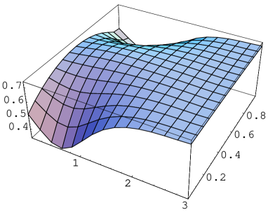
Figure 3: The DEM for $\lambda_{1}(0\leq\lambda_{1}\leq 1)$ and $r(0\leq r\leq 3)$ when the time $t$ is fixed in $t_{r}=2\pi\theta/g$

5 Conclusion

We have studied the influence of the squeezed states on the degree of entanglement which is defined due to mutual entropy for a two-level atom. This shows that the degree of entanglement is very sensitive to the squeezing parameter. For small values of the squeezing parameter, a decrease of the degree of entanglement is shown, while for large values, an increase of the degree of entanglement is obtained. This is manifested in the degree of entanglement as it settles to a constant value for further increasing of the squeezing parameter. This means that one can control the degree of entanglement by using the squeezing. We also found where the degree of entanglement in the JCM for any squeezing parameter $r$ takes the maximum value, applying the mixed states to the initial atomic states. Moreover, we are interested in which the DEM has an upper bound for squeezing parameter $r$. However, from only figure 3, we do not know whether the DEM has an upper bound or goes to infinity. This will remain as the forthcoming problem.

References

- [1] S. Furuichi and M. Ohya, Lett. Math. Phys,49, 279 (1999).
- [2] C. H. Bennett, D. P. Di-Vincenzo, J. A. Smolin and W. K. Wootters, Phys. Rev. A,54, 3824 (1996).
- [3] V. Vedral, M. B. Plenio, M. A. Rippin and P. L. Knight, Phys. Rev. Lett., 78, 2275 (1997).
- [4] J. von Neumann, Mathematische Grundlagen der Quantenmechanik, Springer Berlin, 1932.
- [5] H. Umegaki, Kodai Math. Sem. Rep. 14, 59 (1962).
- [6] M. Ohya and D. Petz, Quantum Entropy and its Use, Sprinver-Verlag, 1993.
- [7] M. Ohya, Rep. Math. Phys. 27, 19 (1989).
-
[8]
V.P.Belavkin and M.Ohya, Quantum entanglements and entangled
mutual entropy,
quant-ph/9812082. - [9] H. Araki and E. H. Lieb, Commun. Math. Phys., 18, 160 (1970).
- [10] E. T. Jaynes and F. W. Cummings, Proc. IEEE, 51, 89 (1963).
- [11] H.-I. Yoo and J. H. Eberly, Phys. Rep. 118, 239 (1985).
- [12] B. W. Shore and P. L. Knight, J. Mod. Opt. 40, 1195 (1993)
- [13] E. B. Davies, Quantum Theory of Open System, Academic Press, 1976.
- [14] M. Ohya, IEEE Trans. Inf. Theory, 29, 770 (1983).
- [15] L.Accardi and M.Ohya, Appl.Math.Optim.,Vol.39,pp33-59(1999).
- [16] S. J. D. Phoenix and P. L. Knight, Annals of Physics, 186, 381 (1988).
- [17] P. Meystre and M. Sargent 3, Elements of Quantum Optics,Springer-Verlag, 1990.
- [18] D. F. Walls and G. J. Milburn, Quantum Optics, Springer-Verlag, 1994.
- [19] W. Schleich and J. A. Wheeler, Nature, 362, 574 (1987).
- [20] G. J. Milburn, Optica ACTA, 31, 671 (1984).