Spin-Space Entanglement Transfer and Quantum Statistics

Abstract

Both the topics of entanglement and particle statistics have aroused enormous research interest since the advent of quantum mechanics. Using two pairs of entangled particles we show that indistinguishability enforces a transfer of entanglement from the internal to the spatial degrees of freedom without any interaction between these degrees of freedom. Moreover, sub-ensembles selected by local measurements of the path will in general have different amounts of entanglement in the internal degrees of freedom depending on the statistics (either fermionic or bosonic) of the particles involved.

Since the advent of quantum mechanics, entanglement has been identified as one of its most peculiar features [1, 2, 3]. This ”excess correlation” has recently become an important resource in quantum information processing [4]. Entanglement is believed to be at the root of the speed-up of quantum computers over their classical counterparts [5], and it also leads to an unconditionally secure quantum cryptographic key exchange [6]. Another fundamental aspect of quantum physics, somewhat neglected in the field of quantum information, is the distinction between two different types of particles, fermions and bosons, manifested through particle statistics (although see [7] and for fermions see [8, 9, 10]). There are at first sight two seemingly “conflicting” views regarding the role of indistinguishability and particle statistics in quantum information processing. On the one hand, these two notions appear to combine to offer “natural” entanglement through forcing the use of symmetrised and anti-symmetrised states (for bosons and fermions respectively), and as we mentioned before, entanglement is generally an advantage for quantum information processing (although see [11]). On the other hand, indistinguishability prevents us from addressing the particles separately which seems to be disadvantage in information processing. In this article we analyze the role of indistinguishability and particle statistics in a simple information processing scenario.

Consider the following situation. Suppose that we have two pairs of qubits (quantum two-level systems), each pair maximally entangled in some internal degree of freedom. If the particles carrying the qubits are of the same type – say bosons – but distinguishable as a result of spatial separation, then we have two units of entanglement (e-bits) in total. All of this entanglement is in the internal degrees of freedom. If we now consider bringing the particles close together and then separating them again, without the internal degrees of freedom ever interacting with the spatial ones, we should expect the whole entanglement to remain in the internal degrees of freedom. Surprisingly, as we demonstrate in this paper, a fraction of the initial entanglement is transferred to the path degrees of freedom of the particles. The fascinating implication is that the transfer of entanglement is imposed by particle indistinguishability and does not involve any controlled operation between the internal and external degrees of freedom (i.e. spin-path interaction), in contrast with the standard entanglement swapping scheme [12]. The prevalent setting for local manipulations of entanglement in quantum information processing either involves explicit interactions between the internal degrees of freedom of two particles, or an interaction of the internal degrees of freedom with some apparatus. Here we introduce a completely different setting in which particle paths are locally mixed without ANY interaction of the internal degrees of freedom with anything else.

Now we turn to describing the exact details of our thought experiment. Imagine the following setup, described in Fig. 1. We have two pairs of identical particles, each pair being maximally entangled in some internal degree of freedom, e.g. the spin, or polarization. In our case, we consider systems with spin one-half, or isomorphic to it. We assume that our setup is symmetrical both horizontally and vertically, where the dotted lines in Fig. 1 show the axis of symmetry. We have to ensure that particles arrive at the beam splitter at the same time. The initial entanglement is between sides 1 and 2. In each pair, the particles fly apart and meet a particle from the other pair at a beam splitter. The paths on the left hand side are labeled $A$ and $C$ respectively before and after the beam splitter. Similarly, paths on the right hand side are labeled $B$ and $D$.

The output states of this setup represent particles in paths $C1$, $D1$, $C2$ and $D2$ with a particular spin state (we note, for instance, that we can have two particles in $C1$ and none in $D1$). Now we show that, although the initial entanglement is only in the internal degrees of freedom, in the final state some of the entanglement has been transferred to the paths. We will refer to this effect as the Spin-Space Entanglement Transfer by local actions only.

In order to calculate what happens in the above setup, we write our initial state in the second quantization formalism:

$$\frac{1}{\sqrt{2}}(a_{A1\uparrow}^{{\dagger}}a_{A2\downarrow}^{{\dagger}}\pm a_{A1\downarrow}^{{\dagger}}a_{A2\uparrow}^{{\dagger}})\frac{1}{\sqrt{2}}(a_{B1\uparrow}^{{\dagger}}a_{B2\downarrow}^{{\dagger}}\pm a_{B1\downarrow}^{{\dagger}}a_{B2\uparrow}^{{\dagger}})|0\rangle,$$ (1)

where $|0\rangle$ is the vacuum state and, for instance, $a_{A1\uparrow}^{{\dagger}}$ is a creation operator describing a particle in path A1 and with spin up. The positive and negative signs in the above equation are necessary in order to take into account all the possible initial states (the singlet and the entangled triplet of spin). We restrict our attention to analyzing one mode per particle only, but our results can be generalized to any number of modes. Due to the symmetry of the problem we only analyze two cases: when the two signs in equation (1) are the same, the $(+,+)$ case, and when they are different, the $(+,-)$ case. Note that initially there is no left-right correlation between spin and space. This is because there is no uncertainty in either the spin or space in the initial state, so by measuring the spatial state one cannot gain any information about the spin state (and vice-versa) in addition to what we knew before the measurement.

The operation of the beam splitter is described by any unitary transformation in $U(2)$ [13]. However, since the overall phase factor has no relevance for entanglement, we can without any loss of generality consider a transformation in $SU(2)$:

$$U=\left[\begin{array}[]{cc}\alpha&\beta\\ -\beta^{*}&\alpha^{*}\\ \end{array}\right],$$ (4)

where $|\alpha|^{2}+|\beta|^{2}=1$. Since we consider entanglement only between sides $1$ and $2$, the beam splitters in fact perform local unitary operations. Hence they cannot change the total entanglement present initially. Also, they only affect the spatial degrees of freedom and are not intrinsically dependent on spin (or polarization). Therefore they are incapable of swapping entanglement from spin (polarization) to space by performing a controlled not operation in the usual fashion [12]. Although the transformation law will be the same for fermions and bosons, they obey different statistics which is why there will be an observable difference in their behaviour in our experiment. For fermions we have the following anti-commutation relation:

$$[a_{i}^{{\dagger}},a_{j}^{{\dagger}}]_{+}=0,$$ (5)

while for bosons we have the commutation relation:

$$[a_{i}^{{\dagger}},a_{j}^{{\dagger}}]_{-}=0,$$ (6)

where $i$ and $j$ are sets of labels. Figs. 2 to 5 present diagramatically the output states for both fermions and bosons. For instance, the first diagram in Fig. 4 represents the following term:

$$(|\alpha|^{2}+|\beta|^{2})^{2}\,(a_{C1\uparrow}^{{\dagger}}a_{D1\uparrow}^{{\dagger}}a_{C2\downarrow}^{{\dagger}}a_{D2\downarrow}^{{\dagger}})|0\rangle.$$ (7)

Note that for each output pair, i.e. both on sides $1$ and $2$, the total spin (or polarization) $S$ can take the values $0$ or $1$. If we consider, without any loss of generality, that the spin is aligned with the $z$ axis, then $|S_{z}|$ – the absolute value of the projection of S along z – can also only take the values $0$ or $1$. We can then divide the total output wave function into these two components, where the spins of the particles in each output pair are respectively anti-aligned or aligned along $z$.

$|S_{z}|=0$ component: there is no difference between fermions and bosons (bearing in mind that the corresponding operators obey different commutation relations). However, there is a difference between the $(+,+)$ case, where we have all possible output terms (see Fig. 2), and the $(+,-)$ case, where some terms never appear (see Fig. 3).

$|S_{z}|=1$ component: there is a difference between the output states for fermions (see Fig. 4) and bosons (see Fig. 5). For both types of particles, the $(+,-)$ case will only introduce a phase difference in some terms.

As a consequence of applying only local unitary operations, the total output wave function should have also two e-bits of entanglement. For clarity, let us consider for the rest of the paper the particular case of $50/50$ beam splitters ($\alpha=1/\sqrt{2},\beta=-i/\sqrt{2}$). To illustrate the spin-space entanglement transfer effect, we look at the $(+,+)$ case for fermions (Figs. 2 and 4). Here, it is clear that the $|S_{z}|=1$ terms give one e-bit of entanglement, solely in the internal degrees of freedom, as the path states are identical. The $|S_{z}|=0$ case gives the other e-bit of entanglement, but this time involving both the internal and external degrees of freedom. Thus we have spin-space entanglement transfer, without any controlled operation between spin and space.

We now show how we can extract space-only entanglement from the total wave function by doing particular measurements on the internal degrees of freedom without revealing any knowledge about the external ones (this is perfectly allowed by quantum mechanics and can be accomplished by passing the particles on each side through a cavity which extends over both the left and the right paths). For example, we can measure the total spin S on both sides (1 and 2) along the $x$ axis and then select the $S_{x}=0$ results. For fermions, the entire wave function is then projected onto:

$$\frac{1}{\sqrt{2}}\left[\frac{1}{\sqrt{2}}\left(|L\rangle_{1}+|R\rangle_{1}\right)\frac{1}{\sqrt{2}}\left(|L\rangle_{2}+|R\rangle_{2}\right)-\frac{1}{\sqrt{2}}|A\rangle_{1}\frac{1}{\sqrt{2}}|A\rangle_{2}\right],$$ (8)

where $|L\rangle_{1,2}$ means left bunching of the particles, respectively for sides $1$ and $2$, $|R\rangle_{1,2}$ right bunching and $|A\rangle_{1,2}$ represents anti-bunching (unormalized state). The bosonic counterpart of the above state is:

$$\frac{1}{\sqrt{2}}\left[\frac{1}{\sqrt{2}}\left(|L\rangle_{1}+|R\rangle_{1}\right)\frac{1}{\sqrt{2}}\left(|L\rangle_{2}+|R\rangle_{2}\right)+\frac{1}{\sqrt{2}}|A\rangle_{1}\frac{1}{\sqrt{2}}|A\rangle_{2}\right].$$ (9)

Both these states have 1 e-bit of entanglement in space and the same outcome probability of $1/2$. Note that since these two states are orthogonal they can be perfectly discriminated, offering an operational way of distinguishing fermions and bosons.

If on the other hand we measure the spatial components of the total wave function, we will find different amounts of entanglement in the internal degrees of freedom of fermions and bosons. For instance, if we select the anti-bunching results, we will obtain the following state for fermions:

$$\frac{1}{\sqrt{3}}\left[\frac{1}{\sqrt{2}}(a_{C1\uparrow}^{{\dagger}}a_{D1\downarrow}^{{\dagger}}+a_{C1\downarrow}^{{\dagger}}a_{D1\uparrow}^{{\dagger}})\frac{1}{\sqrt{2}}(a_{C2\uparrow}^{{\dagger}}a_{D2\downarrow}^{{\dagger}}+a_{C2\downarrow}^{{\dagger}}a_{D2\uparrow}^{{\dagger}})\right.$$ (10)

$$\left.-(a_{C1\uparrow}^{{\dagger}}a_{D1\uparrow}^{{\dagger}}a_{C2\downarrow}^{{\dagger}}a_{D2\downarrow}^{{\dagger}})-(a_{C1\downarrow}^{{\dagger}}a_{D1\downarrow}^{{\dagger}}a_{C2\uparrow}^{{\dagger}}a_{D2\uparrow}^{{\dagger}})\right]|0\rangle,$$ (11)

with an outcome probability of $2/3$ and $\log_{2}3$ units of entanglement, whereas for bosons we will get:

$$\frac{1}{\sqrt{2}}(a_{C1\uparrow}^{{\dagger}}a_{D1\downarrow}^{{\dagger}}-a_{C1\downarrow}^{{\dagger}}a_{D1\uparrow}^{{\dagger}})\frac{1}{\sqrt{2}}(a_{C2\uparrow}^{{\dagger}}a_{D2\downarrow}^{{\dagger}}-a_{C2\downarrow}^{{\dagger}}a_{D2\uparrow}^{{\dagger}})|0\rangle,$$ (12)

with probability $1/3$ and $0$ units of entanglement.

If we select the bunching results, for fermions we will obtain the state:

$$\frac{1}{\sqrt{2}}(a_{C1\uparrow}^{{\dagger}}a_{C1\downarrow}^{{\dagger}}+a_{D1\uparrow}^{{\dagger}}a_{D1\downarrow}^{{\dagger}})\frac{1}{\sqrt{2}}(a_{C2\uparrow}^{{\dagger}}a_{C2\downarrow}^{{\dagger}}+a_{D2\uparrow}^{{\dagger}}a_{D2\downarrow}^{{\dagger}})|0\rangle,$$ (13)

with an outcome probability of $1/3$ and $0$ units of entanglement, and for bosons we will get:

$$\frac{1}{\sqrt{3}}\left[\frac{1}{\sqrt{2}}(a_{C1\uparrow}^{{\dagger}}a_{C1\downarrow}^{{\dagger}}+a_{D1\uparrow}^{{\dagger}}a_{D1\downarrow}^{{\dagger}})\frac{1}{\sqrt{2}}(a_{C2\uparrow}^{{\dagger}}a_{C2\downarrow}^{{\dagger}}+a_{D2\uparrow}^{{\dagger}}a_{D2\downarrow}^{{\dagger}})\right.$$ (14)

$$+\frac{1}{2}(a_{C1\uparrow}^{{\dagger}}a_{C1\uparrow}^{{\dagger}}+a_{D1\uparrow}^{{\dagger}}a_{D1\uparrow}^{{\dagger}})(a_{C2\downarrow}^{{\dagger}}a_{C2\downarrow}^{{\dagger}}+a_{D2\downarrow}^{{\dagger}}a_{D2\downarrow}^{{\dagger}})$$ (15)

$$\left.+\frac{1}{2}(a_{C1\downarrow}^{{\dagger}}a_{C1\downarrow}^{{\dagger}}+a_{D1\downarrow}^{{\dagger}}a_{D1\downarrow}^{{\dagger}})(a_{C2\uparrow}^{{\dagger}}a_{C2\uparrow}^{{\dagger}}+a_{D2\uparrow}^{{\dagger}}a_{D2\uparrow}^{{\dagger}})\right]|0\rangle,$$ (16)

with probability $2/3$ and $\log_{2}3$ units of entanglement. We observe that for a given path selection one type of particles exhibits some entanglement in the internal degrees of freedom, whereas the other exhibits none. In other words, under the same situation, fermions and bosons show a difference in their information processing behaviour. Moreover, measuring this degree of entanglement in the internal degrees of freedom could thus also be an operational way of distinguishing between fermions and bosons.

In this article we have shown that it is possible to transfer entanglement from the internal to the spatial degrees of freedom through local actions using only the effects of particle indistinguishability and quantum statistics, without any interaction between the spin and the path. Moreover, sub-ensembles selected by local measurements of the path will in general have different amounts of entanglement in the internal degrees of freedom depending on the statistics (either fermionic or bosonic) of the particles involved. This establishes a connection between two fundamental notions of quantum physics: entanglement and particle statistics. We intend to present a more detailed and systematic analysis of this setup in a subsequent longer work.

Our analysis suggests further investigation of the consequences and applications of particle statistics in quantum information processing. For example, in some protocols using spin-space entanglement the statistical effects make it unnecessary to have controlled operations, such as using polarization-dependent beam splitters [14]. Other types of statistics (e.g. anyons) can similarly be addressed within our framework. Recent experiments such as [15, 16] suggest that it would be possible to test our results in the near future.

Y.O. acknowledges support from Fundação para a Ciência e a Tecnologia from Portugal. N.P. thanks Elsag S.p.A. for finantial support. V.V. acknowledges support from Hewlett-Packard company, EPSRC and the European Union project EQUIP.

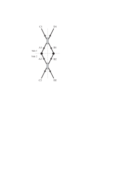
FIG. 1.: This figure presents our setup for spin-space entanglement transfer. Each black circle represents a source of a pair of particles maximally entangled in the internal degrees of freedom (not explicitly shown in the figure). The rectangles represent beam splitters.

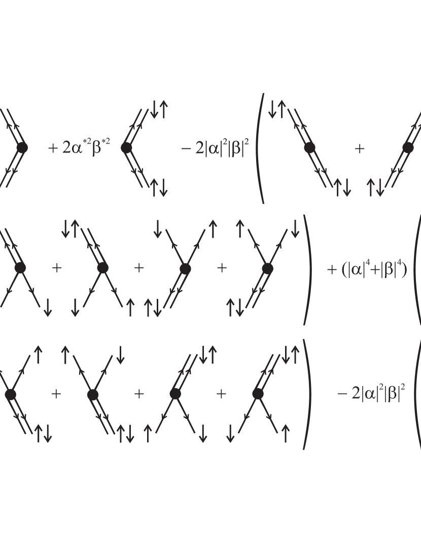
FIG. 2.: Spin $|S_{z}|=0$ component of the total output wave function for the $(+,+)$ case, both for fermions and bosons.

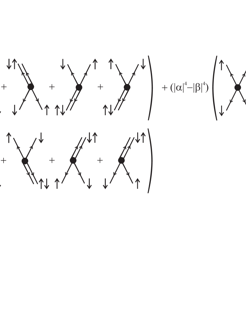
FIG. 3.: Spin $|S_{z}|=0$ component of the total output wave function for the $(+,-)$ case, both for fermions and bosons.

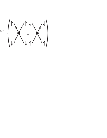
FIG. 4.: Spin $|S_{z}|=1$ component of the total output wave function for the $(+,\pm)$ cases, for fermions.

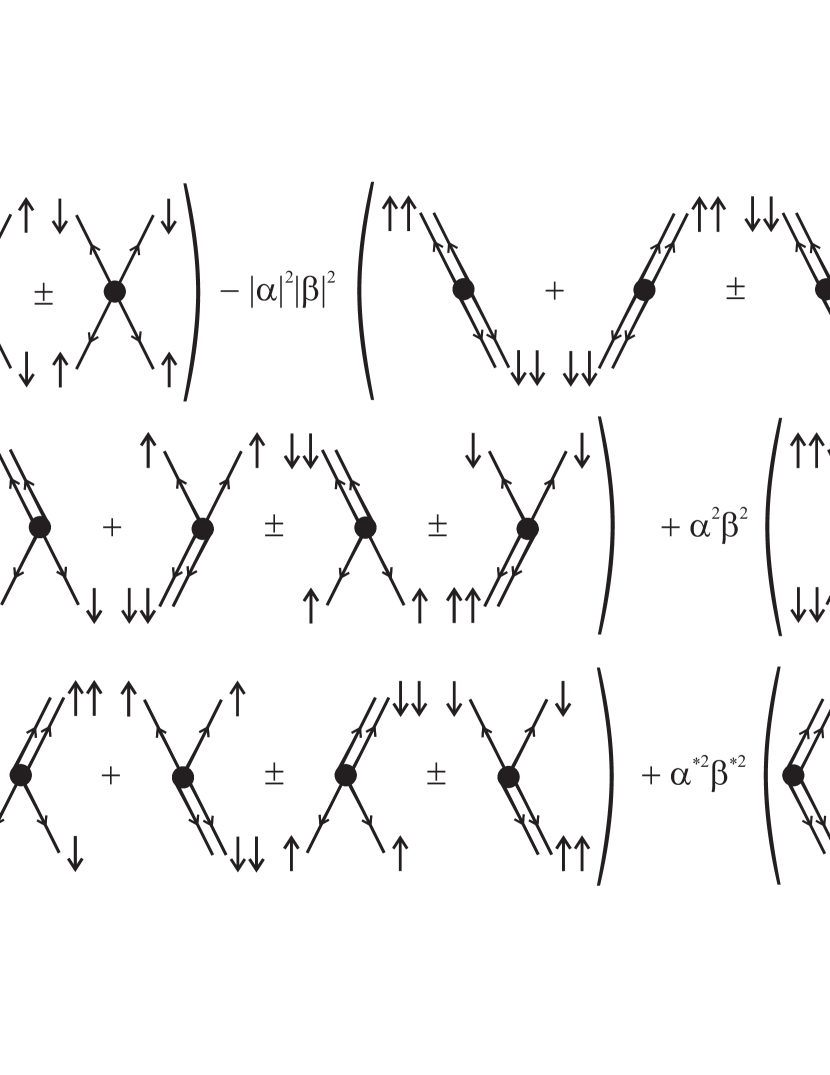
FIG. 5.: Spin $|S_{z}|=1$ component of the total output wave function for the $(+,\pm)$ cases, for bosons.

REFERENCES

- [1] A. Einstein, B. Podolsky and N. Rosen, Phys. Rev. 47, 777 (1935).
- [2] E. Schrödinger, Naturwissenschaften 23, 807, 823, 844 (1935).
- [3] J. Bell, Speakable and Unspeakable in Quantum Mechanics (Cambridge University Press, Cambridge, 1987).
- [4] See for example, A. Steane, Rep. Prog. Phys. 61, 117 (1998).
- [5] P. W. Shor, in Proc. Annual Symposium on Foundations of Computer Science, edited by S. Goldwasser (IEEE Computer Society Press, Nov. 1994) pp. 124-134 (1996); for a review of this algorithm see A. Ekert and R. Jozsa, Rev. Mod. Phys. 68, 733 (1996).
- [6] A. K. Ekert, Phys. Rev. Lett. 67, 661 (1991).
- [7] S. Bose and D. Home, Phys. Rev. Lett. 88, 050401 (2002).
- [8] D. S. Abrams and S. Lloyd, Phys. Rev. Lett. 79, 2586 (1997).
- [9] J. Schliemann, J. I. Cirac, M. Kuś, M. Lewenstein and D. Loss, Phys. Rev. A 64, 022303 (2001); J. Schliemann, D. Loss and A. H. MacDonald, Phys. Rev. B 63, 085311 (2001).
- [10] A. T. Costa Jr. and S. Bose, Phys. Rev. Lett. 87, 277901 (2001).
- [11] F. Herbut and M. Vujičić, J. Phys. A 20, 5555 (1987); F. Herbut, Am. J. Phys. 69 (2), 207 (2001).
- [12] M. Zukowski, A. Zeilinger, M. A. Horne and A. K. Ekert, Phys. Rev. Lett. 71, 4287 (1993); S. Bose, V. Vedral and P. L. Knight, Phys. Rev. A 57, 822 (1998).
- [13] R. Loudon, Phys. Rev. A 58, 4904 (1998).
- [14] Y. Omar, N. Paunković, S. Bose and V. Vedral, arXiv preprint quant-ph/0112004 (2001).
- [15] T. J. Herzog, P. G. Kwiat, H. Weinfurter and A. Zeilinger, Phys. Rev. Lett. 75, 3034 (1995).
- [16] R. C. Liu, B. Odom, Y. Yamamoto and S. Tarucha, Nature 391, 263 (1998).