Quantum Computing with Quantum Dots on Quantum Linear Supports

Abstract

Motivated by the recently demonstrated ability to attach quantum dots to polymers at well-defined locations, we propose a condensed phase analog of the ion trap quantum computer: a scheme for quantum computation using chemically assembled semiconductor nanocrystals attached to a linear support. The linear support is either a molecular string (e.g., DNA) or a nanoscale rod. The phonon modes of the linear support are used as a quantum information bus between the dots. Our scheme offers greater flexibility in optimizing material parameters than the ion trap method, but has additional complications. We discuss the relevant physical parameters, provide a detailed feasibility study, and suggest materials for which quantum computation may be possible with this approach. We find that Si is a potentially promising quantum dot material, already allowing a 5-10 qubits quantum computer to operate with an error threshold of $10^{-3}$.

I Introduction

The tremendous excitement following the discovery of fast quantum algorithms [1, 2] has led to a proliferation of quantum computer proposals, some of which have already been realized in a rudimentary fashion. A representative list includes nuclear spins in liquids [3, 4, 5] and solids [6], trapped ions [7, 8, 9, 10], atoms in microwave cavities [11], atoms in optical lattices [12], atoms in a photonic band gap material [13, 14, 15] , quantum dots [16, 17, 18, 19, 20, 21, 22, 23, 24], donor atoms in silicon [25, 26] and silicon-germanium arrays [27], Josephson junctions [28, 29, 30, 31, 32], electrons floating on helium [33], electrons transported in quantum wires [34, 35], quantum optics [36, 37], quantum Hall systems [38], and anyons [39, 40]. For critical reviews of some of these proposals see [41, 42, 43]. To date, no single system has emerged as a clear leading candidate. Each proposal has its relative merits and flaws with respect to the goal of finding a system which is both scalable and fault tolerant [44], and is at the same time technically feasible. In this paper we examine the possibility of making a solid state analog of a scheme originally proposed for the gas phase, namely trapped ions. One purpose of making such a study is to undertake a critical assessment of both the benefits and the disadvantages which arise on translation of an architecture designed for atomic states coupled by phonons, to the corresponding architecture for condensed phase qubits. Our proposal uses quantum dots (semiconductor nanocrystals) and quantum linear supports (polymers or nanorods) in an ultracold environment. It relies on recent advances in the ability to chemically attach nanocrystals to polymers in precisely defined locations. Quantum dots are coupled through quantized vibrations of the linear support that are induced by off-resonance laser pulses and information is stored in exciton states of the dots. Internal operations on exciton states are accomplished using Raman transitions. We provide here a detailed analysis that allows evaluation of the merits and demerits of a condensed phase rather than gas phase implementation.

Semiconductor nanostructures are known as “quantum dots” (QDs) when their size is of the order of or less than the bulk-exciton Bohr-radius. In such “zero-dimensional” QDs the electron-hole pairs are confined in all three dimensions and the translational symmetry that holds for bulk semiconductors is totally lost. As a result of this quantum confinement the energy-level continuum of the bulk material changes into a discrete level structure. This structure is very sensitively dependent on the QD radius and shape, crystal symmetry, relative dielectric constant (compared to the surrounding medium), surface effects, and defects. This sensitivity can be used to create and control a wide range of optical effects [45]. In general, the term “quantum dot” is used to refer to both “0-dimensional” semiconductor structures embedded within or grown on a larger lattice, i.e., lattice bound, and to individual, chemically assembled semiconductor nanocrystals [46]. QDs can be created in a larger crystal structure by confining a two-dimensional electron gas with electrodes [47], or by making interface fluctuations in quantum wells [48]. A number of promising proposals for quantum computation have been made using the lattice-bound dots [16, 17, 18, 19, 20, 21, 22]. We consider here instead the chemically assembled semiconductor nanocrystals. In the remainder of this paper the term QD will therefore be implicitly understood to refer specifically to chemically assembled nanocrystals.

A large amount of theoretical and experimental information about nanocrystal QDs exists. Nanocrystals have been studied for their photoluminescence properties, linear absorption properties, and non-linear spectroscopy, using a variety of models and techniques[49, 50, 51, 52, 53, 54, 55, 56, 57, 58, 59, 60, 61, 62, 63, 64, 65, 66, 67, 68, 69, 70, 71, 72, 73, 74, 75, 76, 77, 78, 79, 80, 81, 82, 83, 84, 85]. For reviews see, e.g., [86, 87, 88]. These studies clarified the roles of size-dependence, lattice structure, surface effects and environment on the exciton spectrum. However, little attention has been paid so far to the possibility of using nanocrystal QDs for quantum computing. One reason may be the difficulty of coupling nanocrystals. Direct interactions between separate dots are small and difficult to engineer, so that the route to scalability is not obvious. In the only other study to date that proposed to use nanocrystals for quantum computing, Brun and Wang considered a model of nanocrystals attached to a high-Q microsphere and showed that the interaction between QDs can be achieved by using whispering gallery modes of the microsphere to entangle individual qubits [23]. One problem with realization of this model is that only a few QDs can be placed on each microsphere. Therefore, scalability would depend on the ability to connect the microspheres by optical wires.

An exciting route to bypass the coupling problem for quantum dots is suggested by the recently demonstrated ability to attach QDs to polymers by chemical methods at well-defined locations [89]. We show below that at sufficiently low temperatures, the QD-polymer system has quantized vibrational modes that can be used to couple electronic excitations in quantum dots in a controlled and coherent manner. This “quantum information bus” concept derives from the ion trap implementation of quantum computation proposed by Cirac and Zoller [7]. Ion trap schemes take advantage of addressable multilevel ions that are trapped in harmonic wells. The ions are then coupled through interaction with their collective vibrational modes [7]. This scheme can be extended to any system of multilevel quantum objects bound by coupled quantum harmonic oscillators. We apply this approach here to a series of nanocrystal QDs attached to a linear support. The excitonic states of the QD act as carriers of quantum information which are coupled to the vibrational states of the linear support. A linear support is a one-dimensional material (e.g., a stretched polymer or a clamped nanoscale rod) that is connected at each end to a wall. The support is contained in either a vacuum or a non-interacting condensed phase matrix such as liquid helium.

The main advantage of using quantum dots rather than ions is the ability to control the optical properties of quantum dots by varying the size, shape and composition of the dot. On the other hand, a disadvantage is that the analysis for quantum dots is complicated by the fact that they are complex composite objects and are not naturally “clean”. For example, defects and surface effects can influence the electronic properties [90]. Our model presupposes that nanocrystals which are sufficiently “clean” will ultimately be available, so this puts some severe demands on the experimentalist.

Section II gives an outline of the proposal, describing the basic physics and the formal similarities with the ion trap scheme. Section III describes the physics of the qubits, namely the electronic states of quantum dots, and the quantum linear support which provides the information bus between qubits. A summary of the necessary requirements of the qubit states is given here. In Section IV we then show how one-qubit and two-qubit operations can be performed in this system of coupled quantum dots. Section V discusses the feasibility of undertaking quantum logic, with a detailed analysis of the constraints imposed by decoherence and physical parameters. Quantitative estimates are made for several specific candidate systems in Section VI, followed by conclusions and discussion in Section VII.

II Theoretical Overview

We outline here the basic elements of the quantum dot-quantum linear support scheme for quantum computation. The proposed system consists of semiconductor nanocrystal QDs attached at spacings of several tens of nanometers to a quantum linear support (a string or rod). Each QD supports one qubit through a certain choice of excitonic states. Single qubit operations are executed by optical transitions between these states. QDs are coupled by the linear support in analogy to the ion trap scheme [7]. Thus, one uses detuned laser pulses to excite a phonon of the quantum linear support, which can then be used to cause conditional interactions between different dots. The system is depicted schematically in Figure 1. The distance between the quantum dots is assumed to be large relative to their size (see also Section III B and III C.) In the presence of external driving fields, the full Hamiltonian can be written as the sum of three contributions

$\displaystyle H=H_{0}+H_{C}+H_{I},$

where $H_{0}$ is the free Hamiltonian, $H_{C}$ is the coupling Hamiltonian, and $H_{I}$ is the Hamiltonian describing the interaction between the system and the applied laser fields.

The free Hamiltonian, $H_{0}$, is given by

$$H_{0}=\sum_{n=1}^{N}\sum_{j}\hbar\omega_{nj}^{e}|\Psi_{j}\rangle_{n}\langle\Psi_{j}|+\sum_{n=1}^{N}\sum_{k}\hbar\omega_{nk}^{d}b_{nk}^{\dagger}b_{nk}+\sum_{m}\hbar\omega_{m}^{s}a_{m}^{\dagger}a_{m}+\sum_{l}\hbar\omega_{l}^{f}c_{l}^{\dagger}c_{l}.$$ (1)

These four terms represent the energies of the excitons, of the QD phonons, of the linear support phonons, and of the external electromagnetic field, respectively. Here $n$ is the QD index, $|\Psi_{j}\rangle_{n}$ is an exciton eigenstate in the $n^{{\rm th}}$ QD, $b_{nk}$ is an annihilation operator of the $k^{{\rm th}}$ phonon mode of the $n^{{\rm th}}$ QD, $a_{m}$ is an annihilation operator of the $m^{{\rm th}}$ linear support phonon mode, and $c_{l}$ is an annihilation operator of the $l^{{\rm th}}$ mode of the quantized external electromagnetic field. The phonon frequencies of the support are denoted by $\omega^{s}$, and those of the quantum dot by $\omega^{d}$.

The coupling Hamiltonian, $H_{C}$, is given by

$$H_{C}=\sum_{njkl}\beta_{njkl}|\Psi_{j}\rangle_{n}\langle\Psi_{k}|c_{l}^{\dagger}+\sum_{njkl}\gamma_{njik}|\Psi_{j}\rangle_{n}\langle\Psi_{i}|b_{nk}^{\dagger}+\sum_{njkl}\alpha_{nkl}b_{nk}c_{l}^{\dagger}+{\rm H.c.}$$ (2)

The first term is responsible for radiative decay of exciton states. The most important radiative decay pathway is the recombination of the electron and the hole. The second term describes the exciton-phonon interaction and gives rise to both pure dephasing and to non-radiative transitions between exciton states. The third term is a coupling between the QD phonons and the electromagnetic field.

The interaction Hamiltonian $H_{I}$ describes the coupling of the excitons to single-mode plane-wave lasers in a standing wave configuration. We treat the laser fields semi-classically. A QD has a permanent dipole moment due to the different average spatial locations of the electron and hole. In the dipole limit, we can write

$$H_{I} = {\bf D}\cdot{\bf E}$$ (3)

$$= {\sum_{{\bf k}ijn}}\;\left[{}_{n}\langle\Psi_{i}|e{\cal(}{\bf r}_{e}^{n}-{\bf r}_{h}^{n})|\Psi_{j}\rangle_{n}|\Psi_{i}\rangle_{n}\langle\Psi_{j}|\right]\cdot\left[{\bf\epsilon}_{{\bf k}}{\rm E}_{{\bf k}}\sin({\bf k}\cdot{\bf r}_{{\rm cm}}^{n}+\phi_{x}){\rm\cos}(\nu_{{\bf k}}t-\phi_{t})\right].$$ (4)

Here ${\bf r}_{e}^{n}$ and ${\bf r}_{h}^{n}$ are the position vectors of the electron and hole in the $n^{{\rm th}}$ QD respectively; ${\bf r}_{{\rm cm}}^{n}$ is the center of mass location of this QD; ${\bf\epsilon}_{{\bf k}}$ , ${\rm E}_{{\bf k}}$ and $\nu_{{\bf k}}$ are, respectively, the polarization, electric field amplitude, and frequency associated with the field mode ${\bf k}$; $\phi_{x}$ and $\phi_{t}$ are the spatial and temporal phases of the field. The dipole limit is valid here since a typical energy scale for single-particle electronic excitations in QDs is $0.1-1$eV, corresponding to wavelengths $1/k\sim 0.1-1\mu m$. For a typical dot radius $R\leq 5$ nm, the electric field is then almost homogeneous over the dot. In analogy to ion trap schemes [7], the center of mass of the $n^{{\rm th}}$ QD, ${\bf r}_{{\rm cm}}^{n}$, is decomposed into its constituent phonon modes,

$${\bf r}_{{\rm cm}}^{n}=\sum c_{mn}{\bf q}_{m}=\sum c_{mn}{\bf q}_{0m}(a_{m}^{\dagger}+a_{m}),$$ (5)

where ${\bf q}_{m}$ are normal modes and ${\bf q}_{0m}$ is the zero-point displacement for the $m^{{\rm th}}$ normal mode, ${\bf q}_{0m}$ =$\sqrt{\hbar/{2M\omega_{m}}},$ where $M$ is the mass of the mode and $\omega_{m}$ is the mode frequency. For low phonon occupation numbers, where the motion of the center of mass of the QD is small compared to the wavelength of the light, the Lamb-Dicke regime is obtained, i.e.,

$$\eta_{mn{\bf k}}={\bf k}\cdot c_{mn}{\bf q}_{0m}\ll 1.$$ (6)

Therefore, we can expand $H_{I}$ to first order in the Lamb-Dicke parameter $\eta$:

$$H_{I}=2\hbar\sum_{{\bf k}ijn}g_{{\bf k}}^{ijn}|\Psi_{i}\rangle_{n}\langle\Psi_{j}|{\rm\cos}(\nu_{{\bf k}}t-\phi_{t})\left(\sin\phi_{x}+\sum_{m}\eta_{mn{\bf k}}(a_{m}^{\dagger}+a_{m}){\rm\cos}\phi_{x}\right){\rm.}$$ (7)

Here

$$g_{{\bf k}}^{ijn}={{}_{n}}\langle\Psi_{i}|\frac{e{\rm E}_{{\bf k}}}{2\hbar}\epsilon_{{\bf k}}\cdot{\cal(}{\bf r}_{e}^{n}-{\bf r}_{h}^{n})|\Psi_{j}\rangle_{n}$$ (8)

is the resulting coupling parameter between the carrier states in the $n^{{\rm th}}$ QD. The second term in Eq. (7) transfers momentum from the laser field to the QD, thereby exciting phonon modes of the linear support. This term allows us to perform two-qubit operations, as described below. Manipulation of the spatial phase $\phi_{x}$ allows us to selectively excite either the carrier transition, i.e., a change in the internal degrees of freedom of the QD without changing the vibrational state of the support, or a side band transition in which the internal degrees of freedom of both the QD and the vibrational mode of the support are changed, depending on whether our QD is located at the antinode or node of the laser, respectively [9].

Now, let $\Omega=2\pi/\tau_{{\rm op}}$ be the Rabi frequency of our desired quantum operations [see Section IV], and let $T$ be the temperature. Our system must then satisfy the following set of basic requirements:

1. $\tau_{{\rm op}}<\tau_{{\rm rec}}$, where $\tau_{{\rm rec}}$ is the time scale for exciton recombination. Typically $\tau_{{\rm rec}}=10^{-3}-10^{-6}$sec [60, 91].

2. $\Omega<\omega^{s}_{1}$, where $\omega^{s}_{1}$ is the first harmonic of the linear support spectrum. This requirement must be met in order to resolve the individual support modes.

3. $k_{b}T<\hbar\omega^{s}_{1}$. This ensures that only the ground state phonon mode is occupied. This requirement comes from the Cirac-Zoller ion-trap scheme[7], where the motional ground state is used as the information bus.

4. Dephasing and population transfer due to exciton-phonon coupling must be minimized, or preferably avoided altogether.

We now discuss the details of our system in light of these requirements.

III Qubit and Linear Support Definitions

A Definition of Qubits

In analogy to the Cirac-Zoller ion trap scheme [7], three excitonic states will be used, denoted $|0\rangle_{n},|1\rangle_{n},$ and $|2\rangle_{n}$. Very recent advances in ion trap methodology have allowed this requirement to be reduced to only two states [92] (see also [93]). However, for our purposes it suffices to use the more familiar three state scheme. The states $|0\rangle_{n}$ and $|1\rangle_{n}$ are the qubit logic states, and $|2\rangle_{n}$ is an auxiliary state that is used when performing two-qubit operations. These three exciton states must possess the following properties:

1. Dark for optical recombination: This is required so that we will have long recombination lifetimes.

2. Dark for radiative relaxation to other exciton states: This is required to prevent leakage to other exciton states.

3. Degenerate: The energy separation is required to be smaller than the lowest energy internal phonon, in order to suppress nonradiative transitions between states. We wish to make transitions between vibronic eigenstates, rather than creating oscillating wavepackets which would dephase as they move on different potential surfaces. Obtaining a large amplitude for moving between vibrational eigenstates of two surfaces depends on the existence of two features (i) large Frank-Condon overlap [94] between these eigenstates, which will be the case for degenerate exciton potential energy surfaces; and (ii) very narrow-bandwidth laser pulses which can selectively address the required states. These transitions are described in Section IV A. The degeneracy will need to be broken in order to perform certain operations.

In order to choose states which satisfy the above requirements, detailed calculation of the exciton wavefunctions and fine structure of the quantum dots is essential. We employ here the multi-band effective mass model which has been employed by a number of groups for calculation of the band-edge exciton fine structure in semiconductor QDs made of direct band gap semiconductors [52, 60] . For larger nanocrystals, possessing radii $R>20$Å, multi-band effective mass theory is generally in reasonably good agreement with experiment as far as energetics are concerned [73]. It has been used extensively for CdSe nanocrystals by Efros and co-workers [61]. While the effective mass approximation (EMA) has known serious limitations [87], and has been shown not to provide quantitative results for smaller nanocrystals [73], it nevertheless provides a convenient, analytically tractable description, with well defined quantum numbers for individual states, and will allow us to perform an order of magnitude assessment of the feasibility of our scheme.

To explain the exciton state classification resulting from the multi-band EMA, it is necessary to consider a hierarchy of physical effects leading to an assignment of appropriate quantum numbers. These effects are, in decreasing order of importance: (i) quantum confinement (dot of finite radius, typically smaller than the bulk exciton radius), (ii) discrete lattice structure (iii) spin-orbit coupling, (iv) non-spherical nanocrystal geometry, and facetting of surfaces, (v) lattice anisotropy (e.g., hexagonal lattice), (vi) exchange coupling between electron and hole spin. The electron-hole Coulomb interaction is neglected: detailed calculations show that this may be treated perturbatively over the range of nanocrystal sizes for which the EMA is accurate [77, 95]. These effects lead to the following set of quantum numbers: $n_{e}$ ($n_{h}$) the principle electron (hole) quantum number, $J_{e}$ ($J_{h})$ the total electron (hole) angular momentum, $L_{e}$ ($L_{h})$ the lowest angular momentum of the electron (hole) envelope wavefunction, $S_{e}$ ($S_{h})$ the electron (hole) Bloch total angular momentum, and the total angular momentum projection

$$F_{z}=m_{K}+m_{s},$$ (9)

where $m_{K}=\pm 1/2,\pm 3/2,\pm 5/2,..$ refers to the projection of the hole total angular momentum $J_{h}$, and $m_{s}=\pm 1/2,\pm 3/2,\pm 5/2,..$ is the projection of the electron total angular momentum $J_{e}$. State multiplets are classified by $n_{e}L_{eJ_{e}}$ $n_{h}L_{hJ_{h}},$ e.g. $1S_{1/2}1P_{3/2}$, and states within the multiplet are labeled by $F_{z}$. For a II-VI semiconductor such as CdSe, the Bloch states for the valence band hole states possess total angular momentum $S_{h}=3/2,1/2$, deriving from coupling of the local orbital angular momentum $1$ in $p$-orbitals, with hole spin $1/2$. The corresponding Bloch states for the conduction band electron states have total angular momentum $S_{e}=1/2$, deriving from coupling of the local orbital angular momentum $0$ in $s$-orbitals, with electron spin-$1/2$. We consider here only states within the band edge multiplet, for which $L_{e}=L_{h}=0$, and $S_{e}=1/2,S_{h}=3/2$. Hence the total electron and hole angular momenta are given by $J_{e}=1/2,J_{h}=3/2$, respectively and there are a total of eight states within this multiplet. It follows from Eq. (9) that there is one $F_{z}=2$ state, two $F_{z}=1$ states, two $F_{z}=0$ states, two $F_{z}=-1$ states, and one $F_{z}=-2$ state in this $1S_{1/2}1S_{3/2}$ multiplet. States within a doublet are distinguished by a superscript ($L$ or $U$). The eigenfunctions, linear absorption spectrum and selection rules for dipole transitions from the ground state to this lowest lying EMA multiplet are calculated in Ref. [60]. For spherical QDs the following results were found:

• Hexagonal crystal structure: The $F_{z}=\pm 2$ states constitute degenerate exciton ground states. The $F_{z}=\pm 2$ states and one of the $F_{z}=0$ states (denoted $0^{L}$) are optically dark in the dipole approximation.

• Cubic crystal structure: The $F_{z}=0^{L},\pm 1^{L},\pm 2$ states constitute degenerate exciton ground states, and are all optically dark.

We consider here explicitly a nanocrystal made from a direct band gap material with cubic crystal structure. An exciton wavefunction of the $1S_{1/2}1S_{3/2}$ multiplet, $\Psi_{F_{z}}({\bf r}_{e},{\bf r}_{h})$, can be expanded in terms of products of single-particle wavefunctions $\psi_{1/2,m_{s}}^{S}({\bf r}_{e})$ and $\psi_{3/2,m_{K}}^{S}({\bf r}_{h})$ [52, 60]. In order to satisfy the requirement of optically dark qubits (recall condition 1 above), we construct our qubit from the $F_{z}=-2,0^{L}$ states:

$$|0\rangle \equiv |\Psi_{0^{L}}({\bf r}_{e},{\bf r}_{h})\rangle=\frac{1}{\sqrt{2}}\left[|\psi_{1/2,-1/2}^{S}({\bf r}_{e})\psi_{1/2,+1/2}^{S}({\bf r}_{h})\rangle-|\psi_{1/2,+1/2}^{S}({\bf r}_{e})\psi_{3/2,-1/2}^{S}({\bf r}_{h})\rangle\right]$$ (10)

$$|1\rangle \equiv |\Psi_{-2}({\bf r}_{e},{\bf r}_{h})\rangle=|\psi_{1/2,-1/2}^{S}({\bf r}_{e})\psi_{3/2,-3/2}^{S}({\bf r}_{h})\rangle.$$ (11)

The auxiliary level for cycling transitions is taken to be the $F_{z}=2$ state:

$$|2\rangle\equiv|\Psi_{+2}({\bf r}_{e},{\bf r}_{h})\rangle=|\psi_{1/2,+1/2}^{S}({\bf r}_{e})\psi_{3/2,+3/2}^{S}({\bf r}_{h})\rangle.$$ (12)

Explicit expressions for the electron and hole wavefunctions are given in Appendix IX. The states $|0\rangle,|1\rangle,|2\rangle$ are degenerate and have equal parity [determined by $(-1)^{F_{z}}$].

Naturally, for nonspherical, noncubic, and/or indirect band gap materials, other states may be more appropriate. It is only essential that they satisfy the requirements above. In this paper we shall use primarily the EMA states described above for cubic nanocrystals of direct gap materials, because they illuminate in an intuitive and quantifiable manner the difficulties associated with our proposal. However, in the discussion of feasibility (Section V), we will also present results obtained with qubit states obtained from tight binding calculations for nanocrystals constructed from an indirect band gap material (silicon).

B Quantum Linear Support

In order to determine whether quantum computation is possible on such a system we need to examine also the properties of the linear support. The support is made out of $K$ small units, e.g., unit cells or monomers. We can write the displacement of each unit as a sum of normal modes,

$${\bf x}_{k}=\sum_{m}\tilde{c}_{mk}{\bf q}_{m}=\sum_{m}\tilde{c}_{mk}{\bf q}_{0m}(a_{m}^{\dagger}+a_{m}).$$ (13)

The zero point displacements for a homogeneous support are

$${\bf q}_{0m}=\sqrt{\hbar/\left(2\lambda l\omega_{m}\right)},$$ (14)

where $\lambda$ is the linear mass density and $l$ is the length of the unit. The lowest energy modes will be long-wavelength transverse modes. Since the wavelengths of the modes of interest are large compared to the separation between neighboring units, we can approximate the support as being continuous.

In many cases, a sparse number of attached QDs will have only a small effect on the normal modes of the support. The validity of this assumption depends on the materials chosen and will be discussed more thoroughly below. For now we will calculate all of the relevant properties assuming point-like, massless quantum dots, consistent with our assumption that the spacing between the dots is larger relative to their intrinsic size. For the $n^{{\rm th}}$ point-like QD attached to unit cell $k$, with one dot per unit cell, we can identify the dot and cell normal modes expansion coefficients. We then have $c_{mn}\equiv\tilde{c}_{mk}$, where $\tilde{c}_{mk}$ and $c_{mn}$ are, respectively, the coefficients relating the displacement of the $k^{{\rm th}}$ unit cell and $n^{{\rm th}}$ QD to the displacement of the $m^{{\rm th}}$ normal mode [Eqs. (5) and (13), respectively]. For a continuous support, the set of $\tilde{c}_{mk}$ becomes a function $\tilde{c}_{m}(x)$ that is the normalized solution to the wave equation on the support. Any specific value of $c_{mn}$ can now be written $c_{m}(x_{n})$, where $x_{n}$ is the position of the $n^{{\rm th}}$ QD.

The two most common types of linear continuous systems are strings and rods.

1 Strings

In a string, the resistance to transverse motion comes from an applied tension, $\vartheta$. The dispersion relation for the frequency of a string in mode $m$ is

$\displaystyle\omega_{m}^{s}=\sqrt{\frac{\vartheta}{\lambda}}k_{m},$

where $\lambda$ is the linear mass density and $k_{m}$ is the wavenumber. The normalized solution to the transverse wave equation with fixed ends is given by

$\displaystyle c_{m}(x)=\sqrt{\frac{2l}{L}}\sin(k_{m}x),$

where $k_{m}$ = $m\pi/L$, $l$ is the unit length, and $L$ is the string length.

2 Rods

In a rod, the resistance to transverse motion results from internal forces. This leads to a different dispersion relation and, consequently, to a different solution $c_{m}(x)$. The transverse modes of a rod can be defined in terms of the length $L$, density $\rho$, the Young’s modulus $Y$, the cross-sectional area $A$, and the second moment of $A$ (or the massless moment of inertia of a slice of the rod), ${\bf I}$. As shown by Nishiguchi et al. [96], the long wavelength phonon modes ($\lambda\geq 1000$ Å) are well described by the classical dispersion equation

$\displaystyle\omega_{m}^{s}=k_{m}^{2}\sqrt{\frac{YI_{z}}{\lambda A}}.$

where $I_{z}$ is the moment in the direction of the displacement.

The transverse normal modes for a clamped rod are well known [97], resulting in the solution

$$c_{m}(x) = N_{m}\left[\sin(k_{m}L)-\sinh(k_{m}L)\right]\left[\cos(k_{m}x)-\cosh(k_{m}x)\right]$$

$$- \left[\cos(k_{m}x)-\cosh(k_{m}x)\right]\left[\sin(k_{m}L)-\sinh(k_{m}L)\right].$$

Here $N_{m}$ is a normalization constant proportional to $\sqrt{1/L}$. The values of $k_{m}$ are not known analytically, but can be shown to be proportional to $1/L$.

C Approximations

The important parameters characterizing the support are $\omega_{1}^{s}$, the frequency of its first harmonic, and the product

$${\bf S}_{nm}\equiv c_{nm}{\bf q}_{0m}.$$ (15)

This product is the quantum dot displacement resulting from the zero point motion of mode $m$ of the support. We shall refer to it as the dot modal displacement. The above discussion of vibrations in the support assumed massless QDs, motivated by the assumption that they have negligible spatial extent relative to the distance between them. To investigate the effect of the finite mass of the quantum dots, we computed numerical solutions of the coupled vibration equations for strings and rods having finite mass increments located at discrete points, simulating the attachment of finite mass quantum dots. These numerical calculations show that for sparsely spaced dots of mass small enough that the total weight is the same order of magnitude as the weight of the support alone, the resulting value of $S_{nm}$ remains unaffected to within a factor of $2$ by the presence of the dots (see Figure 2). A simple way to approximate the presence of the QDs and retain an analytic solution is then to replace the linear density of the support by the average combined linear density of QD and support.

Since we are interested here in order of magnitude estimates of feasibility, we will approximate $c_{m}(x_{n})$ by $\sqrt{2l/L}.$ This approximation corresponds to the maximum value of $c_{m}(x_{n})$ for a string, and to approximately the maximum value of $c_{m}(x_{n})$ for a rod. Since the larger the dot displacement, the larger the coupling between dots, this means that our estimations of number of operations will be an upper bound.

These approximations combined with Eq. (6) yield the following equation for the Lamb-Dicke parameter,

$$\eta_{m^{\prime}n{\bf k}_{2}}={\bf k}_{2}\cdot{\bf S}_{nm}=k_{2}S_{nm}\cos\theta=k_{2}\sqrt{\frac{\hbar}{M\omega_{m}}}\cos\theta,$$ (16)

where $\theta$ is the angle between the modal displacement and the direction of the laser beam, and $M$ is the total support mass: $M=L\lambda$. Note the inverse power dependence on $M$ in Eq. (16). We shall see in Section V B that the massive nature of the linear support and the resulting small value of the Lamb-Dicke parameter provides the major limitation for our system.

IV Qubit Operations

A One-qubit Operations: Coupling of Dots to Light

1 Derivation of the Interaction Hamiltonian in the Rotating Wave Approximation

While dipole transitions in QDs are similar in principle to dipole transitions in atomic systems, the strong coupling to internal phonon modes adds an additional complexity. Consider the modifications of Eqs. (1)-(4) for a single QD unattached to a linear support, interacting with a single laser field, with the QD located at the anti-node of the field, i.e., with the $\sin({\bf k}\cdot{\bf r}_{{\rm cm}}^{n}+\phi_{x})$ term in Eq. (4) vanishing. Thus, omitting the linear support term:

$\displaystyle H=\sum_{j}\hbar\omega_{j}^{e}|\Psi_{j}\rangle\langle\Psi_{j}|+\sum_{k}\hbar\omega_{k}^{d}b_{k}^{\dagger}b_{k}+\sum_{ijk}\hbar\gamma_{jik}|\Psi_{j}\rangle\langle\Psi_{i}|\left(b_{k}^{\dagger}+b_{k}\right)+\sum_{ij}2\hbar g_{{\bf k}}^{ij}|\Psi_{i}\rangle\langle\Psi_{j}|\cos(\nu_{{\bf k}}t-\phi_{t}).$

We separate this Hamiltonian into two parts, $H_{0}$ and $H_{I}:$

$$H_{0} = \sum_{j}\hbar\omega_{j}^{e}|\Psi_{j}\rangle\langle\Psi_{j}|+\sum_{k}\hbar\omega_{k}^{d}b_{k}^{\dagger}b_{k}+\sum_{jk}\hbar\gamma_{jjk}|\Psi_{j}\rangle\langle\Psi_{j}|(b_{k}^{\dagger}+b_{k})$$ (17)

$$H_{I} = \sum_{i\neq j,k}\hbar\gamma_{jik}|\Psi_{j}\rangle\langle\Psi_{i}|(b_{k}^{\dagger}+b_{k})+\sum_{ij}2\hbar g_{{\bf k}}^{ij}|\Psi_{i}\rangle\langle\Psi_{j}|\cos(\nu_{{\bf k}}t-\phi_{t})$$ (18)

The “free” Hamiltonian $H_{0}$ may be diagonalized by a displacement transformation. Let $D_{k}(\alpha)$ be the unitary displacement operator:

$\displaystyle D_{k}(\alpha)\equiv e^{\alpha b_{k}^{\dagger}-\alpha^{\ast}b_{k}}=D_{k}(-\alpha)^{\dagger}.$

The displaced phonon operator $d_{jk}$ is defined as

$\displaystyle d_{jk}\equiv D_{k}(-\alpha_{jk})b_{k}D_{k}(\alpha_{jk})=b_{k}+\alpha_{jk},$

and satisfies standard boson commutation relations:

$$[d_{jk},d_{j^{\prime}k^{\prime}}^{\dagger}] = \delta_{kk^{\prime}}$$

$$[d_{jk},d_{j^{\prime}k^{\prime}}] = [d_{jk}^{\dagger},d_{j^{\prime}k^{\prime}}^{\dagger}]=0.$$

Note that for real $\alpha_{jk}$ we have $\alpha_{jk}(b_{k}^{\dagger}+b_{k})=d_{jk}^{\dagger}d_{jk}-\alpha_{jk}{}^{2}-b_{k}^{\dagger}b_{k}$. Letting $\alpha_{jk}\equiv\gamma_{jjk}/\omega_{k}^{d}$ and inserting a complete set of exciton states into Eq. (17), we find:

$$H_{0} = \sum_{j}\hbar\omega_{j}^{e}|\Psi_{j}\rangle\langle\Psi_{j}|+\sum_{k}\hbar\omega_{k}^{d}\sum_{j}|\Psi_{j}\rangle\langle\Psi_{j}|\left(b_{k}^{\dagger}b_{k}-\alpha_{jk}(b_{k}^{\dagger}+b_{k})\right)$$

$$= \sum_{j}\hbar\omega_{j}^{e}|\Psi_{j}\rangle\langle\Psi_{j}|+\sum_{jk}\hbar\omega_{k}^{d}|\Psi_{j}\rangle\langle\Psi_{j}|\left(d_{jk}^{\dagger}d_{jk}-\left(\frac{\gamma_{jjk}}{\omega_{k}^{d}}\right)^{2}\right).$$

The eigenstates of $d_{jk}^{\dagger}d_{jk}$ are labeled $|n_{jk}\rangle$ , where $d_{jk}^{\dagger}d_{jk}|n_{jk}\rangle=$ $n|n_{jk}\rangle$ and $\langle n_{jk}|m_{j^{\prime}k^{\prime}}\rangle=\delta_{kk^{\prime}}F_{nmk}^{jj^{\prime}}$. The $F_{nmk}^{jj^{\prime}}$ are Franck-Condon factors [94], describing the overlap of vibrational eigenstates between different excitonic states $j$ and $j^{\prime}$. We can then rewrite $H_{0}$ as

$\displaystyle H_{0}=\sum_{j}\hbar\omega_{j}^{e+}|\Psi_{j}\rangle\langle\Psi_{j}|+\sum_{jk}\hbar\omega_{k}^{d}|\Psi_{j}\rangle\langle\Psi_{j}|d_{jk}^{\dagger}d_{jk},$

where $\omega_{j}^{e+}=\omega_{j}^{e}-\sum_{k}\left(\gamma_{jjk}/\omega_{k}^{d}\right)^{2}$ is the renormalized electronic energy level.

We transform to the interaction picture defined by $H_{0}$: $\widetilde{H}_{I}=\exp\left(iH_{0}t/\hbar\right)H_{I}\exp\left(-iH_{0}t/\hbar\right)$. To do so, it is useful to insert into this expression two complete sets of displaced oscillator states belonging to different excitonic states $i$ and $j$:

$\displaystyle I_{i}\times I_{j}=\bigoplus_{k}\sum_{n}|n_{ik}\rangle\langle n_{ik}|\times\bigoplus_{k^{\prime}}\sum_{m}|m_{jk^{\prime}}\rangle\langle m_{jk^{\prime}}|=\bigoplus_{k}\sum_{nm}|n_{ik}\rangle\langle m_{jk}|F_{nmk}^{ij}.$

Changing variables from $b_{k}$ to $d_{jk}$ in Eq. (18), and transforming to the interaction picture now yields, after some standard algebra:

$$\widetilde{H}_{I} = e^{iH_{0}t/\hbar}H_{I}e^{-iH_{0}t/\hbar}$$ (19)

$$= \sum_{i\neq j,l}\hbar\gamma_{jik}|\Psi_{i}\rangle\langle\Psi_{j}|e^{i\omega_{ij}^{e+}t}\bigotimes_{k\neq l}\sum_{n,m}F_{nmk}^{ij}|n_{ik}\rangle\langle m_{jk}|e^{i\omega_{k}^{d}(n-m)t}$$ (22)

$$\bigotimes_{l}\sum_{n^{\prime},m^{\prime}}F_{n^{\prime}m^{\prime}l}^{ij}\left(-\frac{\gamma_{jjl}}{\omega_{l}^{d}}|n_{il}^{\prime}\rangle\langle m_{jl}^{\prime}|e^{i\omega_{l}^{d}(n^{\prime}-m^{\prime})t}+\sqrt{m^{\prime}+1}|n_{il}^{\prime}\rangle\langle(m^{\prime}+1)_{jl}|e^{i\omega_{l}^{d}(n^{\prime}-m^{\prime}-1)t}\right)$$

$$+\sum_{ij}\hbar g_{{\bf k}}^{ij}|\Psi_{i}\rangle\langle\Psi_{j}|e^{-i(\nu_{{\bf k}}t-\omega_{ij}^{e+}t-\phi_{t})}\bigotimes_{k}\sum_{n,m}F_{nmk}^{ij}|n_{ik}\rangle\langle m_{jk}|e^{i\omega_{k}^{d}(n-m)t}+{\rm H.c.}$$

where $\omega_{ij}^{e+}\equiv\omega_{i}^{e+}-\omega_{j}^{e+}$.

While this expression appears very complicated, it can be drastically simplified under certain reasonable assumptions. First, note that for single-qubit operations we need to consider only two exciton states $|\Psi_{a}\rangle$ and $|\Psi_{b}\rangle$. The first term in $\widetilde{H}_{I}$ essentially describes non-radiative transitions between exciton states due to phonon emission. Under the assumption that the phonon modes are initially unoccupied, we can choose the states $|\Psi_{a}\rangle$ and $|\Psi_{b}\rangle$ such that they have a negligible propensity for nonradiative transitions, i.e., they are protected against single phonon emission (recall condition 3. for “good” qubits in Section III A). This means that we can effectively set all $\gamma_{jik}$ to zero, thus eliminating the first term in $\widetilde{H}_{I}$. This important simplification is treated in detail in Section V A below. Thus we are left with:

$\displaystyle\widetilde{H}_{I}=\hbar g_{{\bf k}}^{ab}|\Psi_{a}\rangle\langle\Psi_{b}|e^{i\phi_{t}-it(\nu_{{\bf k}}-\omega_{ab}^{e+})}\bigotimes_{k}\sum_{n,m}F_{nmk}^{ab}|n_{ak}\rangle\langle m_{bk}|e^{i\omega_{k}^{d}(n-m)t}+{\rm H.c.}$

We then tune our laser on resonance such that $\nu_{k}=\omega_{ab}^{e+}$, and make sure that the laser spectral width is much smaller than the lowest quantum dot phonon frequency, $\omega_{1}^{d}$. This allows us to make the rotating wave approximation (RWA), i.e., eliminate all terms which rotate faster than $\omega_{1}^{d}$, which leads to

$$\widetilde{H}_{I}=\hbar g_{{\bf k}}^{ab}|\Psi_{a}\rangle\langle\Psi_{b}|e^{i\phi_{t}}\bigotimes_{k}\sum_{n}F_{nnk}^{ab}|n_{ak}\rangle\langle n_{bk}|+{\rm H.c}.$$ (23)

This RWA interaction Hamiltonian, Eq. (23), is very similar to the familiar two-level system Hamiltonian used extensively in atomic optics [98]. However, the strength of the interaction is modulated here by the Franck-Condon factors, $F_{nnk}^{ab}$. To allow the simplification of the Hamiltonian from Eq. (22) to Eq. (23) requires a judicious choices of laser intensities and states. In our scheme the occupation $n$ of all phonon modes will be initially zero. Using Eq. (8), it is useful to then introduce the factor

$$\Omega_{{\bf k}}^{ab}=g_{{\bf k}}^{ab}\prod_{k}F_{00k}^{ab}=\sqrt{\frac{2\pi\alpha I_{{\bf k}}}{\hbar}}\prod_{k}F_{00k}^{ab}\langle\Psi_{a}|\epsilon_{{\bf k}}\cdot({\bf r}_{e}-{\bf r}_{h})|\Psi_{b}\rangle,$$ (24)

which corresponds to the Rabi frequency for an on-resonant transition. $I_{{\bf k}}$ is the laser intensity and $\alpha=e^{2}/\left(4\pi\varepsilon_{0}\hbar c\right)$ is the fine structure constant.

2 Raman Transitions

Since we wish to use near degenerate states of equal parity for our qubits, we cannot employ dipole transitions. Hence we use Raman transitions. These connect states of equal parity via a virtual transition to a state with opposite parity. Recall that parity is determined by $(-1)^{F_{z}}$. Suppose we start in the $|1\rangle=|\psi_{1/2,-1/2}^{S}({\bf r}_{e})\psi_{3/2,-3/2}^{S}({\bf r}_{h})\rangle$ state, for which $F_{z}=-2$. We can then make transitions through a virtual level $|v\rangle$ that has opposite parity (e.g., $F_{z}=\pm 1$), to the state $|0\rangle$ having $F_{z}=0$. Figure 3a provides a schematic of the coupled QD-laser field system, showing the levels $|0\rangle$, $|1\rangle$ and $|v\rangle$ together with the fields required to cause a Raman transition. Under the assumptions that only two laser field modes ${\bf k}_{1}$ and ${\bf k}_{2}$ are applied, and in the rotating-wave approximation, the standard theory of Raman transitions [99] leads to the following expression for the Raman-Rabi frequency between an initial state $|i\rangle$ and a final state $|f\rangle$:

$$\Omega_{{\rm Raman}}^{fi{\bf k}_{2}{\bf k}_{1}}=\frac{|\Omega_{{\bf k}_{2}}^{fj}\Omega_{{\bf k}_{1}}^{ji}|}{\Delta}.$$ (25)

Here$\ k_{1}$ and $k_{2}$ are chosen such that the detuning, $\Delta=\omega_{j}-\omega_{i}-\nu_{{\bf k}_{1}}=$ $\omega_{j}-\omega_{f}-\nu_{{\bf k}_{2}}$, $j$ is the index of an intermediate exciton state chosen to provide a minimum value of $\Delta$. For single qubit transitions, both lasers are aligned such that the QD is positioned at antinodes.

For QDs possessing cubic crystal structure and composed of direct band gap materials, we have found it advantageous to use the $F_{z}=1$ and $F_{z}=-1$ states of the $1S_{1/2}1P_{5/2}$ multiplet as the intermediate state. An exciton wavefunction of the $1S_{1/2}1P_{5/2}$ multiplet $\Psi_{F_{z}}^{v}(r_{e},r_{h})$ can be expanded in terms of products of single-particle wavefunctions $\psi_{3/2,m_{s}}^{S}(r_{e})$ and $\psi_{5/2,m_{K}}^{P}(r_{h})$.[52, 60] The intermediate $F_{z}=\pm 1$ virtual states can be written:

$\displaystyle|\Psi_{\pm 1}^{v}({\bf r}_{e},{\bf r}_{h})\rangle=-\frac{1}{\sqrt{3}}\left[|\psi_{1/2,\mp 1/2}^{S}({\bf r}_{e})\psi_{5/2,\pm 3/2}^{P}({\bf r}_{h})\rangle+\sqrt{2}|\psi_{1/2,\pm 1/2}^{S}({\bf r}_{e})\psi_{5/2,\pm 1/2}^{P}({\bf r}_{h})\rangle\right]$

The Raman-Rabi Frequency, $\Omega_{{\rm Raman}}$, can then be adjusted by increasing the electric field intensity and by reducing the detuning from the intermediate level. We will describe in detail in Section V B what range of values of intensity and detuning are allowed.

B Two-qubit Operations: Coupling Quantum Dots, Quantum Supports and Light

Our two-qubit operations are equivalent to those of the Cirac-Zoller scheme [7]. The use of optical Raman transitions to implement this scheme has been extensively explored.[8] In our case, we apply the Hamiltonian of Eq. (7) with two lasers $k_{1}$ and $k_{2}$, of frequency $\nu_{1}$ and $\nu_{2}$ respectively. For two-qubit operations, the quantum dot is centered at an antinode of $k_{1}$ and at a node of $k_{2}$. Switching to the interaction picture and calculating second-order transition probabilities to first order in $\eta,$ one obtains the following effective Hamiltonian:

$$H_{{\rm eff}}^{nfi}=-\hbar\sum_{m}\eta_{mn{\bf k}_{2}}(a_{m}^{\dagger}e^{-i\omega_{m}t}+a_{m}e^{i\omega_{m}t})\Omega_{{\rm Raman}}^{fi{\bf k}_{2}{\bf k}_{1}}|\Psi_{f}\rangle_{n}\langle\Psi_{i}|e^{i(\omega_{f}-\omega_{i})t}e^{-i(\left(\nu_{1}-\nu_{2}\right)t+\phi_{2}-\phi_{1})}+{\rm H.c.}$$ (26)

Note that the nodal and antinodal lasers result in an effective Hamiltonian in which $\eta$ depends only on the nodal laser $k_{2}$. This differs from the effective Hamiltonian derived for Raman transitions when travelling waves are used [8]. The lasers are chosen to have a net red detuning, $\omega_{f}{}-\omega_{i}-\upsilon_{1}+\upsilon_{2}=-\omega_{m^{\prime}}$. In the RWA (i.e., eliminating all terms rotating at $2\omega_{m}$), with $\phi_{2}-\phi_{1}=\pi,$ this yields

$$H_{{\rm eff}}^{nfi}=\Omega_{nm^{\prime}}^{fi{\bf k}_{2}{\bf k}_{1}}|\Psi_{f}\rangle_{n}\langle\Psi_{i}|a_{m^{\prime}}+{\rm H.c.}$$ (27)

where

$$\Omega_{nm^{\prime}}^{fi{\bf k}_{2}{\bf k}_{1}}=\eta_{mn{\bf k}_{2}}\Omega_{{\rm Raman}}^{fi{\bf k}_{2}{\bf k}_{1}}.$$ (28)

This combined QD-linear support operation transfers the $n^{{\rm th}}$ QD from state $i$ to $f$, with an accompanying change of one quantum in the phonon mode $m^{\prime}$ of the support. A schematic representation of this operation for the qubit states $|\psi_{i}\rangle=|0\rangle$ and $|\psi_{f}\rangle=|1\rangle$ is shown in Figure 4. Choosing interaction times such that $t=k\pi/(2\Omega_{nm^{\prime}}^{fi{\bf k}_{2}{\bf k}_{1}})$ where $k$ is an integer specifying the pulse duration, we can write the unitary operator $\exp\left(-\frac{i}{\hbar}H_{{\rm eff}}^{nfi}t\right)=U^{nfi}(t)$ as

$$U_{k}^{nfi}=\exp\left[-i\frac{k\pi}{2}(|\Psi_{f}\rangle_{n}\langle\Psi_{i}|a+{\rm H.c.})\right]$$ (29)

In order for the Cirac-Zoller scheme to be successful, the phonon mode of interest, $m$, must start with zero occupation. The applied operations take advantage of the fact that the zero occupation phonon state is annihilated by the lowering operator: $a|0\rangle=0$. The sequence of unitary operations $U_{{\rm C-phase}}\equiv U_{1}^{n10}U_{2}^{n^{\prime}20}U_{1}^{n10}$ then results in a controlled-phase operation between quantum dots $n$ and $n^{\prime}$, i.e., it causes the second qubit $n^{\prime}$ to gain a phase of $-1$ if the first qubit $n$ is in the $|1\rangle$ state, and no additional phase if the first qubit is in $|0\rangle$. This is equivalent to the matrix operator $I-2|1\rangle_{n^{\prime}}|1\rangle_{n}\ {}_{n^{\prime}}\langle 1|_{n}\langle 1|$. The time required to perform $U_{{\rm C-phase}}$ is then $2\times\left(\frac{\pi}{2}\right)$ for ion $n$ plus $1\times\pi$ for ion $n^{\prime}$, i.e.,

$$\tau_{{\rm C-phase}}\equiv(\Omega_{2}^{nn^{\prime}})^{-1}=\pi(\Omega_{nm^{\prime}}^{fi{\bf k}_{2}{\bf k}_{1}})^{-1}+\pi(\Omega_{n^{\prime}m^{\prime}}^{fi{\bf k}_{2}{\bf k}_{1}})^{-1}$$ (30)

Since the ions $n$ and $n^{\prime}$ are identical we will use the approximation that $\Omega_{nm^{\prime}}^{fi{\bf k}_{2}{\bf k}_{1}}\approx\Omega_{n^{\prime}m^{\prime}}^{fi{\bf k}_{2}{\bf k}_{1}}$ in the remainder of this work, hence

$$\Omega_{2}^{nn^{\prime}}\approx\frac{1}{2\pi}\Omega_{nm^{\prime}}^{fi{\bf k}_{2}{\bf k}_{1}}=\frac{1}{2\pi}\Omega_{2}.$$ (31)

The inverse of the average rate $\Omega_{2}^{nn^{\prime}}$ can then be taken as a measure of the gate time, i.e., of the time for the two-qubit controlled phase operation. We define $\Omega_{2}$ as the sideband interaction strength,

$$\Omega_{2}\simeq\eta_{mn{\bf k}_{2}}\Omega_{{\rm Raman}}^{fi{\bf k}_{2}{\bf k}_{1}}.$$ (32)

Calculation of $\Omega_{{\rm Raman}}^{fi{\bf k}_{2}{\bf k}_{1}}$ was described above in Section IV A [Eq. (25)]. We can obtain the Lamb-Dicke parameter $\eta_{m^{\prime}n{\bf k}_{2}}$ from the decomposition in Eq. (16). This now allows specific evaluation of the contribution from the linear support to the Lamb-Dicke parameter $\eta$. As described in Section III C, we approximate $\eta$ as being independent of the specific dot and from now on will drop the dot index $n$.

C Input and Output

Since the qubit states do not include the ground state of the quantum dot, initialization will generally require a transformation from the ground state of no exciton to the defined qubit state. This can be accomplished by applying magnetic fields which will mix dark and light states allowing for optical transitions. If the magnetic field is then adiabatically removed, one is left with population in the dark exciton state only. Qubit measurements can be made by using a cycling transition, in analogy to ion traps [8].

We conclude this section by summarizing in Fig. 5 the relative energy scales involved in our proposal.

V Feasibility of Quantum Logic

In this section we address in detail the question of the limitations imposed on our system by various physical constraints. We start by considering the issue of decoherence due to coupling of excitons to the internal nanocrystal phonon modes, and propose a solution to this problem. We then study the issues of scaling arising from the trade-off between massiveness of the support, laser intensity, and the need to maintain a large ratio of operations to exciton recombination time. We find that the allowed size of our proposed quantum computer depends on the assumed threshold for fault-tolerant computation.

A Decoherence

According to current analysis of experiments on nanocrystal quantum dots [100], exciton dephasing derives predominantly from the diagonal phonon exciton coupling term of Eq. (2):

$$\sum_{j,k}|j\rangle\langle j|(\gamma_{kj}^{\ast}b_{k}^{\dagger}+\gamma_{kj}b_{k}).$$ (33)

Here $\gamma_{kj}$ is the self-coupling of an exciton state $j$ via phonon $k$, and $b_{k}$ is the lowering operator for the $k^{{\rm th}}$ phonon mode in the ground electronic state. In the ground state the coupling is zero, and all excited electronic states have potential energy surfaces which are shifted with respect to this ground state. We desire to eliminate dephasing due to the first-order phonon exciton interaction. In the typical experimental situations in which dephasing has been studied in the past, dephasing occurs on a timescale of nanoseconds for small dots [100]. This rate is extremely rapid compared to the experimental recombination time of dark states ($\sim 10^{-6}$ s for direct band gap materials such as CdSe[60]). The reason for such fast dephasing is twofold. First, the vibrational stationary state of the first electronic level becomes a moving vibrational wave packet on the upper electronic surface, because the spectral width of the pulse is too broad to distinguish vibrational eigenstates. Second, the QD is embedded in a solid state medium where the vibrations of the nanocrystal are then coupled to vibrations of the larger lattice. The phonons of the QD can be treated as analogous to damped cavity modes in atomic optics[98]. In the case of strong coupling, one finds from numerical simulation that the dephasing between any two states $j$ and $j^{\prime}$ is related to the rate of phonon mode excitation. The latter is proportional to $|\gamma_{kj}-\gamma_{kj^{\prime}}|^{2}$ for each mode $k$ [100]. This conclusion of fast dephasing agrees with the analogous result for a leaky optical cavity[98] as well as with the results of experimental [101] and theoretical [100] analysis for embedded semiconductor nanocrystals.

The dephasing can be reduced in three ways. First, the coupling of the QD phonon modes to external phonon and photon modes can be reduced by judicious choice of nanocrystal geometry and material. In our case the QD can dissipate phonon modes only to the support. In the limit of no coupling to external modes, there will be no dephasing but the time required for recurrences could limit our gate repetition rate. Although the oscillations will be fast, the oscillations for different phonon energies will be incommensurate with one another. This could introduce a slow quantum beating between ground and excited electronic states, which would have the undesirable consequence of requiring gate durations to equal a full beat cycle.

Second, one can find a set of electronic states $|j\rangle$ such that

$$\gamma_{kj}-\gamma_{kj^{\prime}}=0\text{ \ \ }\forall j,j^{\prime},\text{and }\forall k.$$ (34)

Physically this condition represents a set of electronic states which create the same potential energy surface for nuclear motion. This elimination of decoherence by degeneracy is an example of a decoherence-free subspace [102, 103, 104]. The Jahn-Teller effect implies that no two such states should exist, because there will always be a phonon mode which will distinguish between these states due to non-linearity[105]. However, in the linear approximation we have

$$\gamma_{kj}=\langle j|\gamma_{k}({\bf r}_{h})+\gamma_{k}({\bf r}_{e})|j\rangle.$$ (35)

The deformation potential coupling operator, $\gamma_{k}(r)$, is a function of the phonon modes and is expressed as

$$\gamma_{k}({\bf r})\equiv\gamma_{nlm}({\bf r})=E_{d}\nabla\cdot{\bf u}_{nlm}{\bf(r)},$$ (36)

where $E_{d}$ is the deformation potential, and $u_{nlm}(r)$ is the coordinate representation of the normalized spheroidal phonon mode of level $n$ with angular momentum $l$ and projection $m$. Following Takagahara [100], the spheroidal modes can be written as

$${\bf u}_{nlm}{\bf(r)=}\sqrt{\frac{\hbar}{2\rho\omega_{nlm}}}(p_{nl}{\bf L}_{lm}(h_{nl}{\bf r})+q_{nl}{\bf N}_{lm}(k_{nl}{\bf r})),$$ (37)

where $\rho$ is the nanocrystal density, $\omega_{nlm}$ is the frequency of the spherical phonon $nlm$, $L_{lm}(hr)=\frac{1}{h}\nabla\Psi_{lm}(hr)$, $N_{lm}(kr)=\frac{1}{k}\nabla\times\nabla\times r\Psi_{lm}(kr)$, and $\Psi(kr)=j_{l}(kr)Y_{l}^{m}(\Omega)$. $j_{l}\left(r\right)$ is an $l^{{\rm th}}$ order spherical Bessel function, $Y_{l}^{m}(\Omega)$ is a spherical harmonic, $k_{n}$ and $h_{n}$ satisfy stress-free boundary conditions at the surface, and $p_{nl},q_{nl}$ are determined by normalization. One can then write

$$\gamma_{nlm}({\bf r})=-E_{d}\sqrt{\frac{\hbar}{2\rho\omega_{nlm}}}p_{nl}h_{nl}j_{l}(h_{nl}r)Y_{l}^{m}(\Omega).$$ (38)

For a cubic, direct gap nanocrystal, the states $|j\rangle$ are states of well defined angular momentum projection. Since the $Y_{l}^{m}$ in Eq. (38) connects states with equal projection, the only phonon modes which can have non-zero matrix elements in Eq. (35) are those with $m=0$ [106]. The resulting matrix elements will be independent of the sign of the exciton angular momentum projection $F_{z}$ [Eq. (9)], i.e., the $m=0$ phonon modes cannot distinguish between exciton states having $F_{z}$ or $-F_{z}$. Therefore, in the linear approximation, the states$|\Psi_{-2}(r_{e},r_{h})\rangle$ and $|\Psi_{2}(r_{e},r_{h})\rangle$ will not dephase with respect to each other. Recall that we took these states as our qubit state $|1\rangle$ and auxilary state $|2\rangle$ states [Eqs. (11),(12)].

Third, and most importantly, one can change the way in which transitions are made. In the above two situations, the motional wave packet of one electronic surface is transferred to another electronic surface without changing shape, i.e., the Franck-Condon approximation holds. However, such a transition requires either a broad laser or a fast excitation. This is not actually the regime of relevance here. The scheme outlined in this work requires selective excitations of sidebands whose energy separation is orders of magnitude smaller than the quantum dot phonon energies (see Fig. 5). Therefore, we will be performing transitions from one vibrational eigenstate to another vibrational eigenstate. Such transitions were described in Section IV with respect to the ground vibrational state. Consequently, the scheme proposed in this work is not affected by fast phonon dephasing.

Exciton states recombine and thus decay to the ground state by both spontaneous emission of photons and phonons. We denote the recombination lifetime $\tau_{{\rm re}}$. Nanocrystals are known to have dark state recombination times ranging from $10^{-6}$s to $10^{-3}$s, depending on the material chosen [60, 73, 91, 95]. In our system, $\tau_{{\rm re}}$ will be the fastest decoherence time for individual qubits. One could potentially suppress radiative recombination by placing the whole system in a cavity[107].  Classical calculations of Roukes and co-workers show that nanoscale rods at low temperature have high $Q$ values: $Q\geq 10^{10}$ [108]. This implies that the rods are only very weakly coupled to their environments and we can therefore assume that in the quantum regime, the high $Q$ will lead to favorably long decoherence times. Another possible source of decoherence is laser scattering from the support (as opposed to the QDs). The magnitude of scattering is dependent on the difference between the spectra of the quantum dots and the electronic and vibrational modes of the support. A detailed analysis of this potentially important decoherence mechanism is beyond the scope of this paper, due to the many possible materials available for both linear supports and quantum dots. Ideally, one would like to choose a support which has an optical window at the frequencies of the lasers used to perform the qubit operations. Estimations based on the Raman transitions proposed above suggest that this optical window needs to be between 0.1 - 1 eV and possess a minimal width of 0.1 meV. Conversely, one can take advantage of the optical tunability of the QDs via their size to construct a QD of such size that its transitions are compatible with a specific optical window suggested by the material properties of the support.

B Parameter Space

We now explore for what range of physical parameters quantum computation is possible within our proposed scheme, by estimating the two-qubit gate fidelity, ${\cal F}$. This fidelity is defined as the trace overlap between the desired final and the achieved final state: ${\cal F}=\min_{\rho_{0}}{\rm Tr}A\rho_{0}A^{\dagger}B(\rho_{0})$, where $A$ is the exact unitary operator for the gate, $B$ is a superoperator describing the actual evolution of the system which takes the initial density matrix $\rho_{0}$ to a final density matrix $\rho_{f}$, and $\rho_{0}$ ranges over all possible input states. For our two-qubit operations described in Section IV B, the fundamental operation is the population transfer to the red side band, $A=U_{1}^{n10}$[Eq. (29)]. $B$ describes both the unitary evolution caused by application of the lasers and the decoherence due to loss of quantum information to the environment. Note that even without decoherence and unknown laser noise, ${\cal F}$ can still be less than unity, due to deviations from the approximations used to derive $A$. Most importantly, deviations from the rotating wave approximation can lead to unwanted population in spectator states.

The resulting value of ${\cal F}$ is determined by two constraints: the decoherence time of the system and the spectral resolution of the gate. As a result of the use of the phonon bus in the two qubit gate construction, both this proposal and the ion trap proposals [7, 10] have gate times that are dependent on the number of qubits. Therefore the quantity of interest is the fidelity of a sideband operation on an array of $N$ quantum dots. First, we note that ${\cal F}$ is limited by the recombination time of the qubit states, $\tau_{{\rm re}}=1/\Gamma$. Naturally, the recombination time $\tau_{{\rm re}}$ must be larger than the sideband operation time, $\tau_{A}=\pi/(2\Omega_{2})$, if the operation is to be successful. One can then define an upper limit on the fidelity that takes into account the statistically independent recombination of the exciton states of all $N$ quantum dots. This background fidelity assumes that $\tau_{{\rm re}}$ is the same for all $N$ quantum dots and it does not account for errors deriving from the interactions with the driving laser field. The background fidelity is then

$${\cal F}{\cal\approx}1-\frac{\tau_{A}}{\tau_{{\rm re}}}=1-\frac{\pi N\Gamma}{2\Omega_{2}}.$$ (39)

${\cal F}$ is also limited by the spectral resolution. We assume that the difference frequency between the lasers is tuned to be resonant with the energy difference between the two states of interest, Figure 4. The energy difference between the states includes the relative Stokes shift induced by both the lasers and the internal phonons. Omitting the adjustment of the laser frequency for the Stokes shifts will lead to gates of reduced fidelity [109, 110]. The primary concern is that the phonon modes be spectrally resolvable. As described in Section II, the use of nodal and antinodal lasers allows us to transfer population to the vibrational sideband and at the same time forbid population transfer to the carrier, i.e., to the excitonic states of the QD. This constrains the operation frequency $\Omega_{2}$ to be smaller than the separation between phonon modes, $\Delta\omega=\omega_{m+1}^{s}-\omega_{m}^{s}$. For small $m$, and for $\Delta\omega\approx\omega_{1}^{s}$, we can then write this constraint as

$$\Omega_{2}<\omega_{1}^{s}.$$ (40)

The population transfer to the off-resonant state will be of the order of $\frac{4g^{2}}{4g^{2}+(\delta)^{2}}$, the result for a two level system interacting with a periodic perturbation of strength $g$ that is off-resonant by a frequency difference $\delta$ [98]. In our case, $g=\Omega_{2}$ and $\delta=\Delta\omega\approx\omega_{1}^{s}$. However, numerical calculations [109] have shown that the population transfer to the off-resonant state for an ion trap system is more accurately estimated by $2\frac{g^{2}}{4g^{2}+(\delta)^{2}}.$ Note that in Ref. [109] g=$\Omega/2,$ the coupling to the carrier transition, and $\delta=\omega_{z}$, the ion trap mode vibrational frequency. The advantage of the standing wave laser configuration is now apparent. For the travelling wave laser configuration, the population transfer to the off-resonant state is $2\frac{(\Omega_{2}/\eta)^{2}}{4(\Omega_{2}/\eta)^{2}+(\omega_{1}^{s})^{2}}\approx 2\left(\frac{\Omega_{2}}{\eta\omega_{1}^{s}}\right)^{2}$ (or, in the notation of Ref. [109], $\frac{1}{2}\left(\frac{\Omega}{\omega_{z}}\right)^{2}).$ However, in the standing wave configuration, one finds that the population transfer is $2\frac{(\Omega_{2})^{2}}{4(\Omega_{2})^{2}+(\omega_{1}^{s})^{2}}$ $\approx 2\left(\frac{\Omega_{2}}{\omega_{1}^{s}}\right)^{2}$. Since $\eta\ll 1$ the off-resonant population transfer is significantly reduced when one uses the standing wave configuration. We can now write down a fidelity which takes into account both the background fidelity, Eq. (39), and the population loss to the most significant spectator state. The fidelity per sideband operation $A$ is then

$${\cal F}\approx 1-\frac{\pi N\Gamma}{2\Omega_{2}}-2\left(\frac{\Omega_{2}}{\omega_{1}^{s}}\right)^{2}$$ (41)

in the standing wave configuration. We emphasize again that if the laser fields are used in a traveling wave configuration, the fidelity is significantly decreased due to transitions to the carrier state, resulting in ${\cal F}\simeq$ $1-\frac{\pi N\Gamma}{2\Omega_{2}}-4(\frac{\Omega_{2}}{\eta\omega_{1}^{s}})^{2}$.

One can now maximize the fidelity with respect to the coupling strength $\Omega_{2}$ for a sideband operation made on an $N$ qubit array. Since

$$\Omega_{2}^{{\cal F}\max}=\left(\frac{\pi(\omega_{1}^{s})^{2}N\Gamma}{8}\right)^{1/3},$$ (42)

for given $\Gamma$ and $\omega_{1}^{s}$, the maximum fidelity can be written as

$${\cal F}_{\max}{\cal=}1-3\left(\frac{\pi N\Gamma}{2\sqrt{2}\omega_{1}^{s}}\right)^{2/3}.$$ (43)

Evaluation of the optimal operation frequency depends then only on the factors in Eq. (42). Inspection of the contributions to $\Omega_{2}$ [Eq. (32)] shows that the underlying adjustable parameters controlling the fidelity in general, Eq. (41), are the intensities $I_{1}$, $I_{2}$, the detuning $\Delta$, and the Lamb-Dicke parameter $\eta$. However, the schematic shown in Figure 4 shows that there are some additional constraints. Thus, it is essential that the inequality $\omega_{1}^{s}<\Delta<\omega_{1}^{d}$ be satisfied in order to avoid unwanted coupling to both the internal phonons and the linear support phonons. In addition, we require that both $|\Omega_{{\bf k}_{1}}^{ji}|$ and $\eta_{01{\bf k}_{2}}|\Omega_{{\bf k}_{2}}^{fj}|$ are smaller than $\Delta$, in order to avoid populating the intermediate level, $|\Psi_{j}\rangle$. Hence, the internal phonon energies define an energy scale which also constrains our system (see Fig. 5).

Furthermore, combining Eqs. (25), (32), and (42), one finds that

$$|\Omega_{{\bf k}_{1}}^{ji}\eta_{01{\bf k}_{2}}\Omega_{{\bf k}_{2}}^{fj}|=\Delta\left(\frac{\pi(\omega_{1}^{s})^{2}N\Gamma}{8}\right)^{1/3}.$$ (44)

Analysis of three level systems has shown that in order to maximize Raman population transfer between states $|\Psi_{i}\rangle$ and $|\Psi_{f}\rangle$, the coupling strength between $|\Psi_{i}\rangle$ and $|\Psi_{j}\rangle$ and $|\Psi_{f}\rangle$ and $|\Psi_{j}\rangle$ should be equal [99]. In the atomic case this usually implies that the respective Rabi frequencies between electronic states, $|\Omega_{{\bf k}_{1}}^{ji}|$ and $|\Omega_{{\bf k}_{2}}^{fj}|$, are equal. However, in our case, with the use of nodal and anti-nodal lasers and coupling to the support phonons, the equivalent condition is that

$$|\Omega_{{\bf k}_{1}}^{ji}|=\eta_{01{\bf k}_{2}}|\Omega_{{\bf k}_{2}}^{fj}|.$$ (45)

Therefore, manipulation of Eqs. (24), (44) and (45), allows us to determine the intensity values, $I_{1}$ and $I_{2}$, necessary for maximum fidelity operations:

$$I_{1} = \frac{\hbar\Delta}{2\pi\alpha}\left(\frac{\pi(\omega_{1}^{s})^{2}N\Gamma}{8}\right)^{1/3}\frac{1}{|\langle\Psi_{j}|\epsilon_{1}\cdot({\bf r}_{e}-{\bf r}_{h})|\Psi_{i}\rangle\prod_{l}F_{00l}^{ji}|^{2}}$$ (46)

$$I_{2} = \frac{\hbar\Delta}{2\pi\alpha}\left(\frac{\pi(\omega_{1}^{s})^{2}N\Gamma}{8}\right)^{1/3}\frac{1}{\eta_{01{\bf k}_{2}}^{2}}\frac{1}{|\langle\Psi_{f}|\epsilon_{2}\cdot({\bf r}_{e}-{\bf r}_{h})|\Psi_{j}\rangle\prod_{l}F_{00l}^{fj}|^{2}}$$ (47)

$$= \frac{\Delta\lambda L}{2\pi\alpha}\left(\frac{\pi(\omega_{1}^{s})^{5}N\Gamma}{8}\right)^{1/3}\frac{1}{|{\bf k}_{2}{\bf|}^{2}}\frac{1}{|\langle\Psi_{f}|\epsilon_{2}\cdot({\bf r}_{e}-{\bf r}_{h})|\Psi_{j}\rangle\prod_{l}F_{00l}^{fj}|^{2}}$$ (48)

Equations (43) , (46), and (47) summarize the limits to implementation of this quantum dot-quantum linear support scheme. To maximize the fidelity we need to increase the frequency of the phonon bus, $\omega_{1}^{s}$. However, as this frequency increases, the increased intensity necessary to reach the maximum fidelity will lead to unwanted evolutions not considered in our simple fidelity equation, Eq. (43). These unwanted evolutions include quadrupolar excitation to higher electronic states. Such transitions will not be removed by the use of nodal and anti-nodal lasers [9]. Consequently, it is useful to define maximal laser intensities, $I_{1}^{\max}$ and $I_{2}^{\max},$ such that Eq.(43) is valid for $I_{1}<I_{1}^{\max}$ and $I_{2}<I_{2}^{\max}$. Therefore the magnitude of $\omega_{1}^{s}$ is restricted and thereby imposes a constraint on the phonon spectrum of the linear support. Furthermore, scalability is also limited by the additional unwanted evolutions, since the required intensity to achieve maximum fidelity also increases with $N$.

There are also physical constraints on the density and length of the support. We assume that the minimal linear density would be provided by a chain of carbon atoms, for which we estimate $\lambda_{{\rm 0}}$=10 amu/Å. The length of the support, $L$, is determined by the number of QDs, $N$, and by the spatial width of the laser, $l$. Thus for identical dots, we have $L=lN$. One could use QDs having no spectral overlap, obtained by making the dots of sufficiently different sizes, in order to achieve more qubits per unit length.

Notice that when one rewrites $L$ in terms of $N$ that the intensity of the nodal laser, $I_{2},$ has a stronger $N$ dependence than the intensity of the anti-nodal laser, $I_{1}$. Physically, this is due to the increased inertia of the system and is quantified by the Lamb-Dicke parameter $\eta$. From Eq. (6) and Section (III B), $\eta\propto M^{-1/2}$ where $M$ is the total mass of the support, $M=\lambda L,$ so that $I_{2}\propto M$ [Eq.(47)]. This coupled with our expression for the maximal gate fidelity, Eq.(43), yields $I_{2}\propto N^{4/3}$. Note that we have used the Lamb-Dicke parameter consistent with the definition made in Ref. [109] which has an inverse $N$ dependence.

To determine the scalability of our system, we examine the maximum number of QDs which can be sustained by a support having given values of $\omega_{1}^{s}$ and $\lambda/\lambda_{\min},$ and provide an acceptable level of fidelity for the sideband operation, $A=U_{1}^{n10}$. We do this by requiring the following three constraints to be simultaneously satisfied: i) ${\cal F}={\cal F}_{\max}$, ii) $I_{2}\leq I$ ${}_{2}^{\max}$, and iii) ${\cal F}_{\max}>1-\varepsilon,$ where $\varepsilon$ can be thought of as the error rate per gate frequency. The first condition states that maximum gate fidelity, Eq. (43), is achieved given the support and quantum dot parameters $\omega_{1}^{s}$ and $\Gamma$, respectively. The second condition states that the laser frequency $I_{2}$ should not exceed the maximum allowed value (see above). Eq. (47) together with the considerations in the previous paragraph shows that $I_{2}$ is dependent on the number of quantum dots $N$. For the range of parameters considered here, $I_{1}$ is always smaller that $I_{1}^{\max}.$ Hence the maximum number of qubits will be determined by the intensity threshold of the system at a node of the laser field. The third condition ensures that one is able to perform an operations with success greater than a certain threshold value (equal to $1-\varepsilon$). Combining these inequalities leads to limits on the number of qubits for a given system.  Conditions i) and iii) can be manipulated to yield the following constraint on $N$:

$$N\leq\omega_{1}^{s}\left(\frac{2\varepsilon}{3}\right)^{3/2}\frac{1}{\pi\Gamma}.$$ (49)

On the other hand, conditions i) and ii) yield a constraint with an inverse power dependence on $\omega_{1}^{s}$. One finds that:

$$N\leq(\omega_{1}^{s})^{-5/4}(I_{2}^{\max})^{3/4}\left(\frac{8}{\pi\Gamma}\right)^{1/4}\left(\frac{2\pi\alpha}{\Delta\lambda l}|{\bf k}_{2}{\bf|}^{2}|\langle\Psi_{f}|\epsilon_{2}\cdot({\bf r}_{e}-{\bf r}_{h})|\Psi_{j}\rangle\prod_{l}F_{00l}^{fj}|^{2}\right)^{3/4}$$ (50)

One can then analyze $N_{\max}$, the maximum allowed value of $N,$ as a function of the linear support frequency $\omega_{1}^{s}$. The combination of Eqs. (49) and (50) results in a cusped function for $N_{\max}$ and is discussed in detail in Section VI for both a direct band gap semiconductor (CdTe) and an indirect band gap semiconductor (Si).

The above discussion has focused on the fidelity for a single component operation, $A=U_{1}^{n10},$ of the C-phase gate $U_{{\rm C-phase}}\equiv U_{1}^{n10}U_{2}^{n^{\prime}20}U_{1}^{n10}.$ We have termed this a sideband operation fidelity. Similar arguments may be made to derive the full C-phase gate fidelity, resulting in the expression

$${\cal F}_{{\rm C-phase}}{\cal\approx}1-\frac{2\pi N\Gamma}{\Omega_{2}}-4\left(\frac{\Omega_{2}}{\omega_{1}^{s}}\right)^{2}.$$ (51)

This is lower than the sideband operation fidelity, both because of the effect of multiple couplings to spectator states and because of an increased operation duration ($\tau_{{\rm C-phase}}=4\tau_{A}$). In the presentation of numerical results in the next section we shall refer only to the prototypical sideband operation fidelity, ${\cal F}$ of Eq. (41).

VI Numerical Estimates for Specific Nanocrystal Systems

A CdTe

CdTe nanocrystals are an example of direct band gap cubic crystal semiconductors QDs. Using parameters found in Landolt-Bornstein [111], we have performed the calculations summarized in the previous sections, using previous results of Efros [60] and Takagahara [100] for the EMA analysis. Although the dark states have infinite lifetimes in the EMA approximation, both experimental [112] and tight binding calculations for the analogous CdSe system [73] yield radiative recombination rates $\Gamma\sim 10^{6}$.

We analyze here nanocrystals with $R=20$ Å. For this size, the frequency of the lowest internal phonon is $\omega_{1}^{d}=2.45\times 10^{12}$Hz. Assuming a minimal separation of a single order of magnitude between the energy spacings $\omega^{d}$ and $\Delta$, we set $\Delta=10^{11}$Hz. The energy separation between the 1S_1/21S_3/2 and 1S_1/21P_5/2 multiplets is $\sim 0.4$ eV in the EMA, which leads to required wave vectors $k_{1}\simeq k_{2}\simeq 2.1\mu$ m^-1 for the irradiating lasers in the two-qubit gates. For the specific CdTe states introduced above (Section III A), we calculate the dipole moments to be $\langle\Psi_{-1}^{\rm aux}({\bf r}_{e},{\bf r}_{h})|\epsilon_{2}\cdot{\bf r}|0\rangle=0.11$ $R$ , $\ \langle\Psi_{-1}^{\rm aux}({\bf r}_{e},{\bf r}_{h})|\epsilon_{1}\cdot{\bf r}|1\rangle=-0.013$ $R$ where $\epsilon_{2}=\frac{1}{\sqrt{2}}(\widehat{x}+i\widehat{y})$ and $\epsilon_{1}=\frac{1}{\sqrt{2}}(\widehat{x}-i\widehat{y}).$ Furthermore we have calculated the Frank Condon overlap to be $\prod_{l}F_{00l}^{\rm aux0}=0.98$ and $\prod_{l}F_{00l}^{\rm aux1}=$ 0.98. We assume that the spatial width of our lasers is diffraction limited. A reasonable estimate of this width is then $l$ = 3 $\mu$m. At constant frequency, an increase in the number of qubits requires an increase in the laser intensity in order to maintain maximum fidelity operations. We estimate that $I_{2}^{\max}=$ 10¹²W/cm ² is the intensity at which the nonresonant quadrupole interactions begin to rise in CdTe quantum dots. However, the intensity could potentially have stricter limitations depending on the spectra of the specific support chosen. As mentioned above for the range of parameters we have examined, the intensity of the anti-nodal laser is weak enough that it does not lead to unwanted time evolutions.

In Figure 6, $N_{\max}$ is plotted as a function of $\omega_{1}^{s}$ for two linear support densities and for a modest threshold of one error every ten operations ($\varepsilon=0.1$). At low frequencies, Eq (49) limits $N_{\max}$ and increasing the values of $\omega_{1}^{s}$ leads to larger values of $N$ for a fixed ${\cal F}_{\max}$. In contrast, higher frequencies require stronger laser intensities [Eq.(47)] so that eventually the limits on the intensity given in condition ii) begin to reduce the maximum possible number of quantum dots, leading to the turnover in Figure 6. Figure 6 also shows that the optimal value of $N_{\max}$, which we denote by $N_{c}$ , is reduced for larger support densities. In Figure 7, we now plot $N_{c}$ as a function of the error threshold $\varepsilon,$ for a range of linear densities $\lambda$. We see that even for two qubit quantum devices one must allow $\varepsilon>0.02,$ or approximately one error every 50 operations. Even at the modest threshold value, $\varepsilon=0.1,$ one can only support 7 qubits. Clearly, CdTe excitons are thus not a good candidate for scalable qubits within this scheme. The underlying reason is that the recombination time of the dark states, while longer than the operation time, is not sufficiently long to provide high fidelity operations.

B Si

Si and other indirect band gap bulk materials exhibit longer exciton recombination lifetimes than direct band gap materials such as CdTe. Although EMA descriptions of Si nanocrystals exist, many subtleties are required to obtain accurate excitonic states [62]. These have also been calculated in semi-empirical tight binding approaches [95], as well as via pseudopotential methods [77]. The advantage of tight-binding descriptions is that the optical properties of the nanocrystal can be determined with inclusion of realistic surface effects [113]. We estimate the feasibility of using Si nanocrystals here using the detailed Si excitonic band structure previously calculated within a semi-empirical description [95]. In order to suppress phonon emission we choose states which correspond to either the exciton ground state, or lie within the minimal phonon energy of the exciton ground state. The minimal phonon energies $\omega_{0}^{d}$ are taken from EMA calculations made by Takagahara [100], and are approximately equal to 5 meV for a nanocrystal of 20 Å radius. One disadvantage of the tight-binding description is that the states are no longer describable as states with well-defined angular momentum, and the calculation of electron-phonon coupling is not straightforward. Therefore, we employ the EMA analysis of Takagahara for this. The Franck-Condon factors are estimated to be $\sim 0.9$ between electronic states derived from the same multiplet. Calculations and experiments on Si reveal dark states with recombination times of microseconds[95]. Tight binding states lack well defined quantum numbers. However, for spherical dots of 20 Å there are multiple dark states which satisfy our phonon emission criteria [95]. States from these multiplets can be used to form our logic and auxiliary states. Calculated Raman transitions between these states have quantitatively similar values to those obtained for CdTe above.

Given an assumed radiative recombination rate $\Gamma=10^{3}$ [95], we perform an analysis similar to the one above for CdTe. In Figure 8 $N_{\max}$ is plotted as a function of $\omega_{1}^{s}$ for a variety of densities $\lambda$ and a threshold of one error every 10 gates ($\varepsilon=0.1$). Figure 8 implies that one could construct a quantum computer composed of 700 quantum dots if $\varepsilon=0.1$. In Figure 9, the extremum value of $N_{\max}$, $N_{c}$ is plotted as a function of $\varepsilon$ for a range of $\lambda$ values. The results are also summarized in Table 1. One sees that, unlike CdTe, for Si there does now exist the possibility of building a quantum processor that possesses an appreciably lower error rate of $\sim$1 error every thousand gates. Most encouragingly, it seems possible to construct a small quantum information processor (5-10 qubits) with a larger linear support density $10\lambda_{0}$, and an error rate of $\varepsilon\leq 10^{-3}$. Naturally, from an experimental perspective it would probably be more realistic to use a support having a density at least ten times greater than our proposed minimal density $\lambda_{0}$ that was estimated for a pure carbon chain (e.g., DNA [45], carbon nanotubes, etched supports, etc.).

VII Conclusions

We have developed a condensed phase scheme for a quantum computer that is analogous to the gas phase ion trap proposal and have explored the feasibility of implementing this scheme with semiconductor quantum dots coupled by a quantum linear support consisting of a string or rod. We have found that the Cirac-Zoller scheme of qubits coupled by a quantum phonon information bus is also applicable in the solid state, and that there exist some advantages to a condensed phase implementation. One such advantage is that there is a potential for significantly less noise in the information bus than in the corresponding gas phase scheme. Calculations by Roukes and co-workers[108] suggest that much higher $Q$ factors may be found for nanorods than are currently obtainable in ion traps. Clearly the extent of the usefulness of our proposal will be very dependent on the choice of materials. To that end we have analyzed the fidelity for two-qubit operations for several candidate systems, including both direct and indirect gap semiconductor quantum dots. We have presented the results of numerical calculations for implementation of the scheme with CdTe and Si quantum dots, coupled via either quantum strings or rods. While neither of these prototypical direct and indirect band gap materials reaches the level of fidelity and size required for large scale quantum computation, the indirect gap quantum dots (Si) do show a reasonably high fidelity with an array of a few tens of dots.

One very revealing result of these explicit calculations of fidelity for one- and two-qubit gates is the limited scalability. The scheme initially appears highly scalable in concept due to the solid-state based architecture. However the detailed analysis given here showed that the dependence of the Lamb-Dicke parameter $\eta$ on the mass of the support is a basic problem which essentially limits the scalability to a few tens of qubits even in the more favorable indirect gap materials. The main drawback of this condensed phase scheme over the ion trap scheme is therefore the large reduction in $\eta$ deriving from the introduction of massive supports. Such a reduction has two important consequences. First, the laser intensities need to be increasingly large to perform operations faster than the decoherence time. Second, such large laser intensities necessitate the use of nodal and antinodal lasers [9, 109]. Without these features, the probability of gate error is extremely high due to transitions to the carrier. This means that several of the alternative schemes proposed for ion trap computation[10, 110] would not provide feasible condensed phase analogs (although the recent scheme of Childs and Chuang[92] which allows computation with two-level ions (or quantum dots) by using both the blue and red sidebands could also be feasible in the condensed phase).

Additional sources of decoherence which have been neglected here (scattering off the support, vibrational and electronic transitions in the support) will also act to limit the number of operations. However one source of decoherence which can be eliminated or at least reduced, is dephasing from the coupling to phonon modes of the support. This is a consequence of the requirement of extremely narrow band-width lasers, and therefore implies that a similar lack of dephasing will hold for other optical experiments on quantum dots which use narrow band-widths. One such example is the proposal to couple quantum dots via whispering gallery modes of glass microspheres [23]. More generally, this result offers a route to avoid dephasing for other spectral measurements on quantum dots[114].

An interesting additional application for this proposal is the laser cooling of nanorods. A single QD could be placed or even etched on a nanostructure. A laser tuned to the red support phonon side band of a QD excited electronic state would excite the energy of the nanocrystal, and at the same time lower the average phonon occupation of the support. When the unstable state relaxes, the most probable transition is the carrier transition. The net result is that the emitted phonon is blue shifted compared to the excitation pulse. The extra energy carried away by the emitted photon is thereby removed from the motional energy of the QD.

The essential physical problem encountered in this condensed phase realization of the qubits coupled by phonon modes is the recombination lifetime of the qubit states, i.e., the exciton radiative lifetime. In principle this could be ameliorated by using hyperfine states of a doped nanocrystal. Recent experimental results demonstrating electronic doping of semiconductor quantum dots offer a potential route to controlled access of these states [115]. The feasibility study presented in this paper does indicate that although the detailed physics of the qubits and their coupling is considerably more complicated in the condensed phase than in the gas phase, limited quantum computation may be possible with phonon-coupled solid state qubits. Further analysis and development of suitable nanoscale architectures and materials is therefore warranted.

VIII Acknowledgments

This work was supported in part by the National Security Agency (NSA) and Advanced Research and Development Activity (ARDA) under Army Research Office (ARO) contracts DAAG55-98-1-0371 and DAAD19-00-1-0380. The work of KRB was also supported by the Fannie and John Hertz Foundation. We thank Dave Bacon and Dr. Kevin Leung for useful discussions.

IX Appendix: Coordinate Representation of Electron and Hole States

We give here the coordinate representation of the electron and hole states. These states were derived in [60] (We employ a slightly different phase convention. Efros et al. when calculating the exchange Hamiltonian, $\gamma S_{h}\cdot S_{e}$, between the hole and electron spin, $S_{h}$ and $S_{e}$, use the convention, $S_{h}\cdot S_{e}=S_{h}^{z}S_{e}^{z}+\frac{i}{2}(S_{h}^{+}S_{e}^{-}-S_{h}^{-}S_{e}^{+})$. We instead use the convention that $S_{h}\cdot S_{e}=S_{h}^{z}S_{e}^{z}+\frac{1}{2}(S_{h}^{+}S_{e}^{-}+S_{h}^{-}S_{e}^{+})$ ). For convenience, we repeat the definitions of our qubit states [Eq. (11)] in slightly more detailed notation:

$$|0\rangle = |\Psi_{1/2,1/2}^{S}({\bf r}_{e})\rangle|\Psi_{3/2,3/2}^{S}({\bf r}_{h})\rangle$$

$$|1\rangle = |\Psi_{1/2,-1/2}^{S}({\bf r}_{e})\rangle|\Psi_{3/2,-3/2}^{S}({\bf r}_{h})\rangle$$

$$|2\rangle = \frac{1}{\sqrt{2}}\left[|\Psi_{1/2,-1/2}^{S}({\bf r}_{e})\rangle|\Psi_{3/2,1/2}^{S}({\bf r}_{h})\rangle-|\Psi_{1/2,1/2}^{S}({\bf r}_{e})\rangle|\Psi_{3/2,-1/2}^{S}({\bf r}_{h})\rangle\right].$$

The electron states are simply the solutions to a free spin-$1/2$ particle in a spherical hard-wall box:

$$|S_{e}\rangle\equiv|\Psi_{1/2,\pm 1/2}^{S}({\bf r})\rangle=\sqrt{\frac{2}{R}}\frac{\sin(\pi r/R)}{r}Y_{0}^{0}(\theta,\varphi)|S,\pm\frac{1}{2}\rangle$$ (52)

where $R$ is the radius of the dot, and $Y_{l}^{m}$ are spherical harmonics. $S$ is a conduction band Bloch function and $\pm\frac{1}{2}$ is the $z$ -projection of the electron spin:

$$|S,\pm\frac{1}{2}\rangle=|L=0,m_{L}=0\rangle|m_{s}=\pm\frac{1}{2}\rangle.$$ (53)

The holes states can be written explicitly as:

$$|\Psi_{3/2,\pm 1/2}^{S}({\bf r})\rangle = -R_{0}(r)Y_{0}^{0}|u_{\pm 1/2}\rangle-R_{2}(r)\left(\sqrt{\frac{2}{5}}Y_{2}^{\pm 2}|u_{\mp 3/2}\rangle+\sqrt{\frac{2}{5}}Y_{2}^{\mp 1}|u_{\pm 3/2}\rangle-\sqrt{\frac{1}{5}}Y_{2}^{0}|u_{\pm 1/2}\rangle\right)|\Psi_{3/2,\pm 3/2}^{S}({\bf r})\rangle$$

$$= -R_{0}(r)Y_{0}^{0}|u_{\pm 3/2}\rangle-R_{2}(r)\left(\sqrt{\frac{2}{5}}Y_{2}^{\pm 2}|u_{\mp 1/2}\rangle-\sqrt{\frac{2}{5}}Y_{2}^{\pm 1}|u_{\pm 1/2}\rangle+\sqrt{\frac{1}{5}}Y_{2}^{0}|u_{\pm 3/2}\rangle\right)$$

where $R_{l}$ are the envelope functions and $|u_{m_{J}}\rangle$ are the valence band Bloch functions.

The radial functions are:

$$R_{2}(r) = \frac{A}{R^{3/2}}\left[j_{2}(\phi r/R)+\frac{j_{0}(\phi)}{j_{0}(\phi\sqrt{\beta})}j_{2}(\phi\sqrt{\beta}r/R)\right]$$

$$R_{0}(r) = \frac{A}{R^{3/2}}\left[j_{0}(\phi r/R)-\frac{j_{0}(\phi)}{j_{0}(\phi\sqrt{\beta})}j_{0}(\phi\sqrt{\beta}r/R)\right]$$

where $j_{l}$ are spherical Bessel functions, $\beta=m_{lh}/m_{hh}$ is the ratio of the light to heavy hole masses, and $\phi$ is the first root of the equation

$\displaystyle j_{0}(\phi)j_{2}(\sqrt{\beta}\phi)+j_{2}(\phi)j_{0}(\sqrt{\beta}\phi)=0.$

The constant $A$ is defined by the normalization condition

$\displaystyle\int_{0}^{R}\left[R_{0}^{2}(r)+R_{2}^{2}(r)\right]r^{2}dr=1.$

The valence band Bloch functions are given by:

$$|u_{\pm 3/2}\rangle = |L=1,m_{L}=\pm 1\rangle|m_{s}=\pm 1/2\rangle$$

$$|u_{\pm 1/2}\rangle = \frac{1}{\sqrt{3}}\left[\sqrt{2}|L=1,m_{L}=0\rangle|m_{s}=\pm 1/2\rangle+|L=1,m_{L}=\pm 1\rangle|m_{s}=\mp 1/2\rangle\right].$$

For our Raman transitions scheme, we have used states which were not analyzed in [60]. In particular, these states are from the $1S_{e}1P_{5/2}$ exciton multiplet. To find these we used techniques developed in [116], and then calculated the eigenstates of the exchange coupling using the method of [60]. A Raman transition connects states of equal parity through a state of opposite parity. Therefore, the states of interest to us are the $F_{z}=\pm 1$ state:

$\displaystyle|\Psi_{\pm 1}^{v}\rangle=-\frac{1}{\sqrt{3}}\left[|\Psi_{1/2,\mp|1/2}^{S}({\bf r}_{e})\rangle|\Psi_{5/2,\pm 3/2}^{P}({\bf r}_{h})\rangle+\sqrt{2}|\Psi_{1/2,\pm 1/2}^{S}({\bf r}_{e})\rangle|\Psi_{5/2,\pm 1/2}^{P}({\bf r}_{h})\rangle\right].$

The electron state is as above. The hole state can be written explicitly as

$$|\Psi_{5/2,\pm 3/2}^{P}({\bf r})\rangle = R_{1}(r)\left(\sqrt{\frac{2}{5}}Y_{1}^{0}|u_{\pm 3/2}\rangle+\sqrt{\frac{3}{5}}Y_{1}^{\pm 1}|u_{\pm 1/2}\rangle\right)$$

$$+R_{3}(r)\left(3\sqrt{\frac{1}{35}}Y_{3}^{0}|u_{3\pm/2}\rangle-\frac{1}{2}\sqrt{\frac{7}{5}}Y_{3}^{\pm 1}|u_{\pm 1/2}\rangle+\sqrt{\frac{1}{14}}Y_{3}^{\pm 2}|u_{\mp 1/2}\rangle+\frac{3}{2}\sqrt{\frac{1}{7}}Y_{3}^{\pm 3}|u_{\mp 3/2}\rangle\right)$$

$$|\Psi_{5/2,\pm 1/2}^{P}({\bf r})\rangle = R_{1}(r)\left(\sqrt{\frac{1}{10}}Y_{1}^{\mp 1}|u_{\pm 3/2}\rangle\sqrt{\frac{3}{5}}Y_{1}^{0}|u_{\pm 1/2}\rangle+\sqrt{\frac{3}{10}}Y_{1}^{\pm 1}|u_{\mp 1/2}\rangle\right)$$

$$+R_{3}(r)\left(3\sqrt{\frac{3}{70}}Y_{3}^{\mp 1}|u_{\pm 3/2}\rangle-\sqrt{\frac{6}{35}}Y_{3}^{0}|u_{\pm 1/2}\rangle-\sqrt{\frac{1}{70}}Y_{3}^{\pm 1}|u_{\mp 1/2}\rangle+\sqrt{\frac{3}{7}}Y_{3}^{\pm 2}|u_{\mp 3/2}\rangle\right),$$

where $R_{l}$ are the envelope functions and $|u_{m_{J}}\rangle$ are the valence band Bloch functions given above.

The radial functions are

$$R_{3}(r) = \frac{B}{R^{3/2}}\left[j_{3}(\phi^{\prime}r/R)+\frac{2j_{1}(\phi^{\prime})}{3j_{1}(\phi^{\prime}\sqrt{\beta})}j_{3}(\phi^{\prime}\sqrt{\beta}r/R)\right]$$

$$R_{1}(r) = \frac{B}{R^{3/2}}\left[j_{1}(\phi^{\prime}r/R)-\frac{j_{1}(\phi^{\prime})}{j_{1}(\phi^{\prime}\sqrt{\beta})}j_{1}(\phi^{\prime}\sqrt{\beta}r/R)\right],$$

where $\phi^{\prime}$ is the first root of the equation

$$j_{1}(\phi)j_{3}(\sqrt{\beta}\phi)+\frac{2}{3}j_{1}(\phi)j_{3}(\sqrt{\beta}\phi)=0$$ (54)

and $B$ is defined by the normalization condition

$$\int_{0}^{R}\left(R_{1}^{2}(r)+R_{3}^{2}(r)\right)r^{2}dr=1.$$ (55)

Table 1. For a given error threshold, $\varepsilon$, and support density $\lambda$, the table shows the optimal value of $N_{\max},N_{c}$ for CdTe and Si nanocrystals. $\lambda_{0}=10$ mu/Å.

-$\log_{10}$($\varepsilon$)	$\lambda/\lambda_{0}$	$N_{c}$(CdTe)	$N_{c}$(Si)
1	1	7	731
	10	3	339
	100	1	158
2	1	1	107
	10	0	50
	100	0	23
3	1	0	16
	10	0	7

FIG. 1.: Schematic visualization of $N$ quantum dots attached to a linear support composed of a nano-scale rod or molecular string. Each quantum dot is addressed by a different laser. The absorption of the dots can be tuned by varying their sizes, allowing selective addressibility with lasers of different wavelengths.

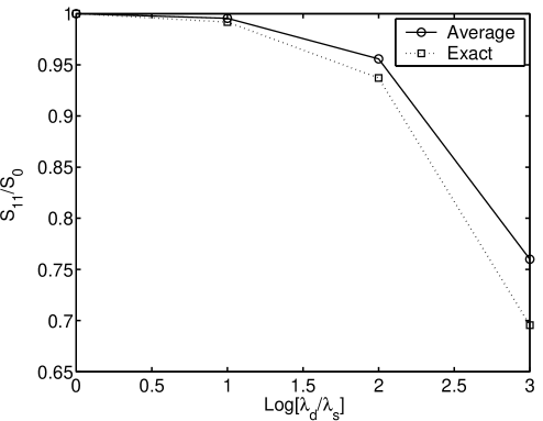
FIG. 2.: The addition of a sparse number of quantum dots to the linear support has relatively little effect on the dot modal displacement $S_{nm}$. Here we present results for $S_{11}$, the dot displacement resulting from the first harmonic of the support, for a system with two QDs attached to a string of length $L=2000$ nm. The QDs are centered at 499 and 1501 nm. Each QD is represented as an increased density that is distributed over a length of 2 nm, e.g., 499 $\pm 2$ nm. Each dot experiences a displacement which is affected by the addition of the second dot on the support. The dot displacement measured relative to the value obtained from a homogeneous string ($S_{0}$), is plotted as a function of $\log((\lambda_{d}+\lambda_{s})/\lambda_{s}$), where $\lambda_{d}$ is the linear density increment due to the dot and $\lambda_{s}$ the linear density of the string. The solid line guides the eye through the exact solution, the dotted line through the solutions obtained for a homogenous density equal to the average of $\lambda_{d}$ and $\lambda_{s}$. One sees that the value of $S_{11}$ changes by less than a factor of 2 over three orders of magnitude change in the normalized average density $(\lambda_{d}+\lambda_{s})/\lambda_{s}$.

FIG. 3.: Energy level scheme for a quantum dot showing the laser fields and transitions necessary for one-qubit operations. (Energy level spacings are not to scale.) Levels $|0\rangle$ and $|1\rangle$ constitute the qubit. The auxiliary level $|2\rangle$ is not involved in these transitions and is not shown. The linear support modes are not involved either. Two antinodal lasers, ${\bf k}_{1}$ and ${\bf k}_{2}$, allow us to perform a Raman transition via a virtual state $|v\rangle$. Transitions occur without changing internal phonon number, since the lasers frequency widths are smaller than the internal phonon frequency, $\omega_{1}^{d}$.

FIG. 4.: Energy level scheme for a quantum dot on the linear support showing laser fields necessary for implementation of two-qubit operations. As described in the text, the use of nodal and antinodal lasers allows us to selectively transfer population from $|0\rangle$ to the lowest energy phonon sideband of $|1\rangle$ (labelled $|1\rangle|s_{1}\rangle$) via a Raman transition, without transferring population to the carrier. The minimum phonon frequency is denoted $\omega_{1}^{s}$. Non-resonant transitions to higher energy phonon sidebands, ($|1\rangle|s_{2}\rangle$) constitute the main source of error in the proposed gates. For very high laser intensities, non-resonant quadrupolar transitions to higher level states (represented by the state $|q\rangle$) also become important.

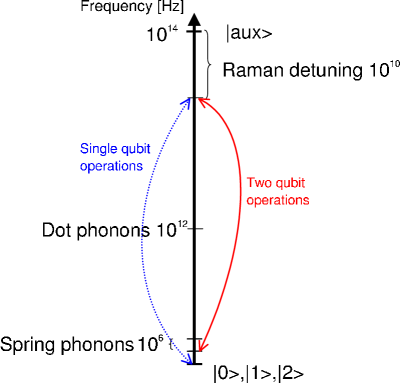
FIG. 5.: Summary of energy scales involved in our proposal for single- and two-qubit operations. The states $|0\rangle$,$|1\rangle$, and $|2\rangle$ appear degenerate on the scale of this figure.

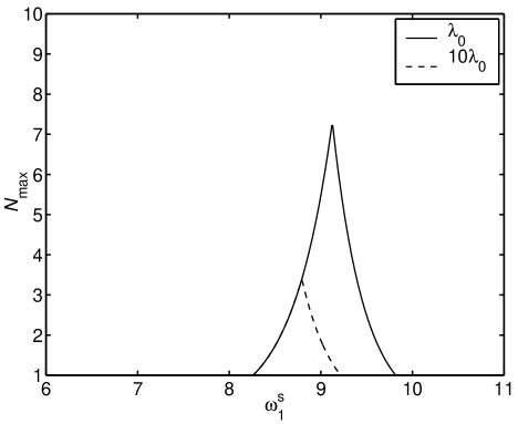
FIG. 6.: Dependence of the maximum number of 20 ÅCdTe nanocrystal quantum dot qubits for which quantum computation is sustainable, subject to the three conditions determined by analysis of the two-qubit gate (see text): i) the fidelity per gate, ${\cal F}={\cal F}_{\max}$, ii) the antinodal laser intensity, $I_{2}\leq I$ ${}_{2}^{\max}$, and iii) ${\cal F}_{\max}>1-\varepsilon,$ where $\varepsilon$ can be thought of as the error rate per gate frequency. The figure shows a plot of $N_{\rm max}$ as a function of the frequency of the linear support phonon mode, $\omega_{1}^{s}$, for two values of the linear support densities, $\lambda_{0}=10$ $\frac{\rm amu}{\text{\AA}}$, $\lambda=10\lambda_{0}$ and $\varepsilon=0.1$. The extremum of the functions corresponds to the maximum possible scalability achievable for 20 Å CdTe nanocrystal qubits. For larger values of $\omega_{1}^{s}$, the larger values of ${\cal F}^{max}$ which are possible in principle are offset by the need for higher intensity lasers. In this situation it is possible to support more qubits than are shown here by relaxing the first constraint. However one thereby loses the advantage of the increase in ${\cal F}_{\max}$ as $\omega_{1}^{s}$ is increased.

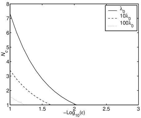
FIG. 7.: Dependence of the optimal number of CdTe nanocrystals, $N_{c}$, (peaks in Fig 6) on the error threshold $\epsilon$ plotted for various linear support densities. $\lambda_{0}=10$ $\frac{\rm amu}{\text{\AA}}$.

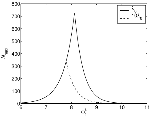
FIG. 8.: Dependence of the maximum number of 20 Å Si nanocrystal quantum dot qubits for which quantum computation is sustainable, subject to the three conditions determined by analysis of the two-qubit gate (see text): i) the fidelity per gate, ${\cal F}={\cal F}_{\max}$, ii) the antinodal laser intensity, $I_{2}\leq I$ ${}_{2}^{\max}$, and iii) ${\cal F}_{\max}>1-\varepsilon,$ where $\varepsilon$ can be thought of as the error rate per gate frequency. The figure shows a plot of $N_{\rm max}$ as a function of the frequency of the linear support phonon mode, $\omega_{1}^{s}$, for two values of the linear support densities, $\lambda_{\rm min}=10$ $\frac{\rm amu}{\text{\AA}}$ and $\lambda=10\lambda_{\rm min}$ and $\varepsilon=0.1$. The extremum of the functions corresponds to the maximum possible scalability achievable for 20 Å Si nanocrystal qubits. The degree of scalability is greater for the indirect band gap material than for the direct band gap CdTe nanocrystals shown in Figure 6, and shows less dependence on the linear support density $\lambda$.

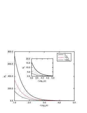
FIG. 9.: Dependence of the optimal numer of Si nanocrystals, $N_{c}$, (peaks in Fig 8) on the error threshold $\epsilon$ plotted for various linear support densities. $\lambda_{0}=10$ $\frac{\rm amu}{\text{\AA}}$.

REFERENCES

- [1] P.W. Shor, SIAM J. on Comp. 26, 1484 (1997).
- [2] L.K. Grover, Phys. Rev. Lett. 79, 325 (1997).
- [3] D.G. Cory, A.F. Fahmy and T.F. Havel, Proc. Nat. Acad. Sci. USA 94, 1634 (1997).
- [4] N. Gershenfeld and I.L. Chuang, Science 275, 350 (1997).
- [5] D.G. Cory, R. Laflamme, E. Knill, L. Viola, T.F. Havel, N. Boulant, G. Boutis, E. Fortunato, S. Lloyd, R. Martinez, C. Negrevergne, M. Pravia, Y. Sharf, G. Teklemariam, Y.S. Weinstein, W.H. Zurek, Fortschrite Der Physik-Progress of Physics 48, 875 (200).
- [6] F. Yamaguchi and Y. Yamamoto, Appl. Phys. A 68, 1 (1999).
- [7] J.I. Cirac and P. Zoller, Phys. Rev. Lett. 74, 4091 (1995).
- [8] D. J. Wineland, C. Monroe, W. M. Itano, D. Leibfried, B. E. King, and D. M. Meekhof, J. of Res. of the National Inst. of Standards and Technology 103, 259 (1998), http://nvl.nist.gov/pub/nistpubs/jres/103/3/cnt103-3.htm.
- [9] D.F.V. James, Appl. Phys. B 66, 181 (1998).
- [10] A. Sorensen and K. Molmer, Phys. Rev. Lett. 82, 1971 (1999).
- [11] Q.A. Turchette, C.J. Hood, W. Lange, H. Mabuchi and H.J. Kimble, Phys. Rev. Lett. 75, 4710 (1995).
- [12] G.K. Brennen, C.M. Caves, P.S. Jessen and I.H. Deutsch, Phys. Rev. Lett. 82, 1060 (1999).
- [13] M. Woldeyohannes and S. John, Phys. Rev. A 60, 5046 (1999).
- [14] N. Vata, T. Rudolph, and S. John, Quantum information processing in localized modes of light within a photonic band-gap material, eprint quant-ph/9910046.
- [15] B. Qiao and H.E. Ruda, J. Appl. Phys. 86, 5237 (1999).
- [16] D. Loss and D.P. DiVincenzo, Phys. Rev. A 57, 120 (1998).
- [17] G. Burkard, D. Loss and D.P. DiVincenzo, Phys. Rev. B 59, 2070 (1999).
- [18] X. Hu and S. Das Sarma, Phys. Rev. A 61, 062301 (2000).
- [19] P. Zanardi and F. Rossi, Phys. Rev. Lett. 81, 4752 (1998).
- [20] A. Imamoglu, D.D. Awschalom, G. Burkard, D.P. DiVincenzo, D. Loss, M. Sherwin and A. Small, Phys. Rev. Lett. 83, 4204 (1999).
- [21] S. Bandyopadhyay, Phys. Rev. B 61, 13813 (2000).
- [22] T. Tanamoto, Phys. Rev. A 61, 022305 (2000).
- [23] T.A. Brun and H. Wang, Phys. Rev. A 61, 032307 (2000).
- [24] E. Biolatti, R.C. Iotti, P. Zanardi, and F. Rossi, Phys. Rev. Lett. 85, 5647 (2000).
- [25] B.E. Kane, Nature 393, 133 (1998).
- [26] G.P. Berman, G.D. Doolen, P.C. Hammel, and V.I. Tsifrinovich, Phys. Rev. Lett. 86, 2894 (2001).
- [27] R. Vrijen, E. Yablonovitch, K. Wang, H.W. Jiang, A. Balandin, V. Roychowdhury, T. Mor, and D. DiVincenzo, Phys. Rev. A 62, 012306 (2000).
- [28] A. Shnirman, G. Schön, and Z. Hermon, Phys. Rev. Lett. 79, 2371 (1997).
- [29] L.B. Ioffe, V.B. Geshkenbeim, M.V. Feigel’man, A.L. Fauchère, and G. Blatter, Nature 398, 679 (1999).
- [30] J.E. Mooij, T.P. Orlando, L. Levitov, L. Tian, C.H. v.d. Wal, and S. Lloyd, Science 285, 1036 (1999).
- [31] Y. Makhlin, G. Schön, and A. Shnirman, Comp. Phys. Commun. 127, 156 (2000).
- [32] A. Blais and A.M. Zagoskin, Phys. Rev. A 61, 042308 (2000).
- [33] P.M. Platzman and M.I. Dykman, Science 284, 1967 (1999).
- [34] R. Ionicioiu, G. Amaratunga, and F. Udrea, Ballistic Single-Electron Quputer, eprint quant-ph/9907043.
- [35] A. Bertoni, P. Bordone, R. Brunetti, C. Jacoboni, and S. Reggiani, Phys. Rev. Lett. 84, 5912 (2000).
- [36] J.D. Franson, Phys. Rev. Lett. 78, 3852 (1997).
- [37] E. Knill, R. Laflamme, and G.J. Milburn, Nature 409, 46 (2001).
- [38] V. Privman, I.D. Vagner, and G. Kventsel, Phys. Lett. A 239, 141 (1998).
- [39] A.Yu. Kitaev, Fault-tolerant quantum computation by anyons, eprint quant-ph/9707021.
- [40] S. Lloyd, Quantum computation with abelian anyons, eprint quant-ph/0004010.
- [41] H.E. Brandt, Prog. in Quantum Electronics 22, 257 (1998).
- [42] D.P. DiVincenzo, Fortschrite Der Physik-Progress of Physics 48, 771 (200).
- [43] M.A. Nielsen and I.L. Chuang, Quantum Computation and Quantum Information (Cambridge University Press, Cambridge, UK, 2000).
- [44] J. Preskill, Proc. Roy. Soc. London Ser. A 454, 385 (1998).
- [45] A.P. Alivisatos, Science 271, 933 (1996).
- [46] L. Jacak, P. Hawrylak, and A. Wójs, Quantum Dots (Springer, Berlin, 1998).
- [47] S.M. Maurer, S.R. Patel, C.M. Marcus, C.I. Duruoz, J.S. Harris Jr., Phys. Rev. Lett. 83, 1403 (1999).
- [48] N.H. Bonadeo, J. Erland, D. Gammon, D. Park, D.S. Katzer, D.G. Steel, Science 282, 1473 (1998).
- [49] Al. L. Efros and A.L. Efros, Sov. Phys. Semicond. 16, 772 (1982).
- [50] L.E. Brus, J. Chem. Phys. 80, 4403 (1984).
- [51] A.I. Ekimov, A.A. Onushchenko, A.G. Plukhin, and Al. L. Efros, Sov. Phys. JETP 61, 891 (1985).
- [52] J. B. Xia, Phys. Rev. B 40, 8500 (1989).
- [53] Y.Z. Hu, M. Lindberg and S.W. Koch, Phys. Rev. B 42, 1713 (1990).
- [54] K.J. Vahala and P.C. Sercel, Phys. Rev. Lett. 65, 239 (1990).
- [55] P.C. Sercel and K.J. Vahala, Phys. Rev. B 42, 3690 (1990).
- [56] A.I. Ekimov, F. Hache, M.C. Schanne-Klein, D. Ricard, C. Flytzanis, I.A. Kudryavtsev, T.V. Yazeva, A.V. Rodina, and Al. L. Efros, J. Opt. Soc. Am. B 10, 100 (1993).
- [57] T. Takagahara, Phys. Rev. B 47, 4569 (1993).
- [58] Al. L. Efros, Phys. Rev. B 46, 7448 (1992).
- [59] Al. L. Efros and A. V. Rodina, Phys. Rev. B 47, 10005 (1993).
- [60] Al. L. Efros, M. Rosen, M. Kuno, M. Nirmal, D. J. Norris, M. Bawendi, Phys. Rev. B 54, 4843 (1996).
- [61] D.J. Norris, Al. L. Efros, M. Rosen, and M.G. Bawendi, Phys. Rev. B 53, 16347 (1996).
- [62] M.S. Hybertsen, Phys. Rev. Lett. 72, 1514 (1994).
- [63] M. Nirmal, D.J. Norris, M. Kuno, M.G. Bawendi, Al. L. Efros, and M. Rosen, Phys. Rev. Lett. 75, 3728 (1995).
- [64] M. E. Schmidt, S. A. Blanton, M. A. Hines, P. Guyot-Sionnest, Phys. Rev. B 53, 12629 (1996).
- [65] U. Banin, C. J. Lee, A. A. Guzelian, A. V. Kadavanich, A. P. Alivisatos, W. Jaskolski, G. W. Bryant, Al. L. Efros, and M. Rosen, J. Chem. Phys. 109, 2306 (1998).
- [66] J.-B Xia and J. Li, Phys. Rev. B 60, 11540 (1999).
- [67] J. Li and J.-B Xia, Phys. Rev. B 61, 15880 (2000).
- [68] Y. Wang and N. Herron, Phys. Rev. B 42, 7253 (1990).
- [69] P.E. Lippens and M. Lannoo, Phys. Rev. B 41, 6079 (1990).
- [70] H.H. von Grunberg, Phys. Rev. B 55, 2293 (1997).
- [71] N.A. Hill and K.B. Whaley, Phys. Rev. Lett. 75, 1130 (1995).
- [72] N.A. Hill and K.B. Whaley, Chem. Phys. 210, 117 (1996).
- [73] K. Leung, S. Pokrant, and K.B. Whaley, Phys. Rev. B 57, 12291 (1998).
- [74] K. Leung and K.B. Whaley, Phys. Rev. B 56, 7455 (1997).
- [75] M.V. Rama Krishna and R.A. Friesner, Phys. Rev. Lett. 67, 629 (1991).
- [76] M.V. Rama Krishna and R.A. Friesner, J. Chem. Phys. 95, 8309 (1991).
- [77] L.-W. Wang and A. Zunger, J. Phys. C 98, 2158 (1994).
- [78] L.W. Wang and A. Zunger, Phys. Rev. B 53, 9579 (1996).
- [79] E. Rabani, B. Hetényi, B.J. Berne, and L.E. Brus, J. Chem. Phys. 110, 5355 (1999).
- [80] B. Delley and E.F. Steigmeier, Appl. Phys. Letters 67, 2370 (1995).
- [81] G.T. Einevoll, Phys. Rev. B 45, 3410 (1992).
- [82] U.E.H. Laheld and G.T. Einevoll, Phys. Rev. B 55, 5184 (1997).
- [83] Y. Ohfuti and K. Cho, J. of Luminescence 70, 203 (1996).
- [84] D.J. Norris and M.G. Bawendi, Phys. Rev. B 53, 16338 (1996).
- [85] S.A. Empedocles and M.G. Bawendi, Science 278, 2114 (1997).
- [86] A.I. Ekimov, J. of Luminescence 70, 1 (1996).
- [87] M. Lannoo, C. Delerue, and G. Allan, J. of Luminescence 70, 170 (1996).
- [88] S.A. Empedocles, R. Neuhauser, K. Shimizu, and M.G. Bawendi, Advanced Materials 11, 1243 (1999).
- [89] A. P. Alivisatos, K. P. Johnson, X. Peng, T. E. Wilson, C. J. Loweth, M. P. Bruchez, P. G. Schultz, Nature 382, 609 (1996).
- [90] M. Kuno, J.K. Lee, B.O. Daboussi, C.V. Mikulec, and M.G. Bawendi, J. Chem. Phys. 106, 9869 (1997).
- [91] H. Heckler, D. Kovalev, G. Polisski, N.N. Zinovev, and F. Koch, Phys. Rev. B 60, 7718 (1999).
- [92] A. M. Childs, and I. L. Chuang, Phys. Rev. A 63, 012306 (2001).
- [93] C. Monroe, D. Leibfried, B.E. King, D.M. Meekhof, W.M. Itano, and D.J. Wineland, Phys. Rev. A 55, R2489 (1997).
- [94] H. Haken and H.C. Wolf, Molecular Physics and Elements of Quantum Chemistry (Springer, Berlin, 1995).
- [95] K. Leung and K.B. Whaley, Phys. Rev. B 56, 7455 (1997).
- [96] N. Nishiguchi, Y. Ando, and N.M. Wybourne, J. Phys.: Condens. Matter 9, 5751 (1997).
- [97] L. D. Landau and E. M. Lifshitz, Theory of elasticity, No. 7 in Course of Theoretical Physics (Butterworth Heinemann, Oxford, 1998).
- [98] M. O. Scully and M. S. Zubairy, Quantum Optics (Cambridge University Press, Cambridge, 1997).
- [99] I. Murray Sargent and P. Horowitz, Phys. Rev. A 13, 1962 (1976).
- [100] T. Takagahara, J. of Luminescence 70, 129 (1996).
- [101] U. Banin, G. Cerullo, A.A. Guzelian, C.J. Bardeen, A.P. Alivisatos and C.V. Shank, Phys. Rev. B 55, 7059 (1997).
- [102] L.-M Duan and G.-C. Guo, Phys. Rev. Lett. 79, 1953 (1997).
- [103] P. Zanardi and M. Rasetti, Phys. Rev. Lett. 79, 3306 (1997).
- [104] D.A. Lidar, I.L. Chuang and K.B. Whaley, Phys. Rev. Lett. 81, 2594 (1998).
- [105] P. R. Bunker and P. Jensen, Molecular Symmetry and Spectroscopy (NRC Research Press, Ottawa, 1998).
- [106] M.E. Rose, Elementary Theory of Angular Momentum (Dover, New York, 1995).
- [107] Jin-Sheng Peng, Gao-Xiang Li, Peng Zhou, and S. Swain, Phys. Rev. A 61, 63807 (2000).
- [108] R. Lifshitz and M.L. Roukes, Phys. Rev. B 61, 5600 (2000).
- [109] A. Steane, C.F. Roos, D. Stevens, A. Mundt, D. Leibfried, F. Schmidt-Kaler, and R. Blatt, Phys. Rev. A 62, 042305 (2000).
- [110] M. P. D. Jonathan and P. Knight, Fast quantum gates for cold trapped ions., eprint quant-ph/0008065.
- [111] L. H, Landolt-Bornstein (Springer-Verlag, Berlin, 1994).
- [112] A.M. Kapitonov, A.P. Stupack, S.V. Gaponenko,E.P. Petrov, A.L. Rogach, A. Eychmuller, J. Phys. Chem. B 103, 10109 (1999).
- [113] K.Leung and K. B. Whaley, J. Chem. Phys. 110, 1012 (1999).
- [114] K.R. Brown and K.B. Whaley, unpublished.
- [115] M. Shim and P. Guyot-Sionnest, Nature 407, 981 (2000).
- [116] G.B. Grigoryan, E.M. Kazaryan, Al. L. Efros, and T.V. Yazeva, Sov. Phys. Solid State 32, 1031 (1990).