How many photons are needed to distinguish two transparencies?

Abstract

We give a bound on the minimum number of photons that must be absorbed by any quantum protocol to distinguish between two transparencies. We show how a quantum Zeno method in which the angle of rotation is varied at each iteration can attain this bound in certain situations.

Making images of objects plays an important part in present day science and technology. In certain situations the object may be damaged by the radiation used to make the image. This can happen, for example, in various types of microscopy of biological specimens.

The simplest way to make an image is to send light through the object and measure how much is absorbed and how much is transmitted. However by using the quantum properties of light and in particular using interferometric techniques one can hope to decrease the amount of radiation absorbed by the object. This question has attracted considerable attention recently [1, 2, 3, 4, 5, 6, 7, 8].

In this paper we shall consider the particular problem of distinguishing two transparencies. This problem is sufficiently simple that it allows detailed analytical treatment but is also sufficiently general that it gives a clear insight into the advantages quantum interferometric techniques can bring to minimal absorption measurements.

Thus suppose there are two objects, with amplitudes for transmission of light $\alpha_{1}$ and $\alpha_{2}$. For instance $\alpha_{1}$ ($\alpha_{2}$) could correspond to the presence (absence) of features with distinctive density in a microscope preparation. Furthermore we shall suppose that there are known prior probabilities $p_{1}$ and $p_{2}$ for objects 1 and 2, respectively. Then it will be shown that the mean number of absorbed photons $\bar{N}^{abs}$ needed by any quantum protocol to distinguish the two objects must satisfy the following bound:

$${\bar{N}^{abs}}\geq{2|\beta_{1}\beta_{2}|\left(\sqrt{p_{1}p_{2}}-\sqrt{P_{E}(1-P_{E})}\right)\over(|1-\bar{\alpha}_{1}\alpha_{2}|-|\beta_{1}\beta_{2}|)},$$ (1)

where $\beta_{i}$ is the amplitude for absorption by object $i$ (so $|\alpha_{i}|^{2}+|\beta_{i}|^{2}=1$ for $i=1,2$), and $P_{E}$ is the probability of error. For instance, this tells us that, with equal prior probabilities and $P_{E}=0$, at least 175 photons must be absorbed in order to distinguish $\alpha_{1}=0.2$ and $\alpha_{2}=0.3$, and at least 2.3 photons to distinguish $\alpha_{1}=0.2$ and $\alpha_{2}=0.8$.

We have also shown, using numerical analyis, that this bound can be approached arbitrarily closely in the case where $\alpha_{1}$ and $\alpha_{2}$ are real, and when the prior probabilties are equal ($p_{1}=p_{2}=1/2$).

When the two transparencies are very close, the dependance of our bound on $\alpha_{1}$ and $\alpha_{2}$, for fixed $P_{E}$, is similar to that derived from classical counting of absorbed photons or simple interferometric techniques [6]. But quantum algorithms have the noteworthy feature that they allow zero error probability. When one of the $\alpha_{i}$ is zero, our bound is zero, and one is in the domain of “interaction-free” measurement [1], where the probability of photon absorption can be made arbitrarily small [9, 2, 3, 5]. Our new bound is interesting in that it spans the entire range from almost identical transparencies to “interaction-free” measurement.

We now turn to the proof of our bound. We follow [6] and write the Hilbert space of a general quantum protocol as a product of three subspaces $H_{A}\otimes H_{P}\otimes H_{O}$. $H_{A}$ is the space of ancillary photons which do not interact with the object and $H_{P}$ the Fock space of the interrogating photons which are directed through the object (for instance, $H_{A}$ corresponds to the empty arm and $H_{P}$ to the object arm in the usual “interaction-free” measurement scheme). $H_{O}$ is the space of the object, with states $|n_{1},\ldots,n_{j},\ldots\rangle_{O}$ if $n_{1},\ldots n_{j},\ldots$ photons have been absorbed by the object at stages $1,\ldots,j,\dots$ of the protocol. If object $i$ is present, the state at step $j$ of the protocol can be written

$$|\Psi^{j}_{i}\rangle=\sum_{k,m,\bf n}C^{j}_{i,km\bf n}|k\rangle_{{}_{A}}|m\rangle_{{}_{P}}|n_{1},\ldots n_{j-1},0_{j},0_{j+1},\ldots\rangle_{{}_{O}},$$ (2)

where $|k\rangle_{{}_{A}}$ denotes $k$ ancillary photons, $|m\rangle_{{}_{P}}$, $m$ interrogating photons and where the sum over ${n_{1},\ldots,n_{j}-1}$, $\sum_{n_{1},\ldots,n_{j}-1}$, has been shortened to $\sum_{\bf n}$. The protocol is assumed to consist of a sequence of unitary steps acting on the joint subspace $H_{A}\otimes H_{P}$, alternating with steps where the interrogating photons interact with the object. Finally, a measurement is carried out whose result indicates which object is present.

The absolute value of the overlap $f^{j}$,

$$f^{j}=|\langle\Psi^{j}_{1}|\Psi^{j}_{2}\rangle|=|\sum_{k,m,\bf n}(\overline{C}_{1}^{j}C^{j}_{2})_{mk\bf n}|.$$ (3)

between the states for objects 1 and 2 measures how effectively the protocol can distinguish the two objects at step $j$. The overlap $f^{j}$ is not altered by unitary steps, of course, but is by interaction steps. The interaction step for object $i$ can be described by $a^{\dagger}_{P}\rightarrow\alpha_{i}a^{\dagger}_{P}+\beta_{i}b^{\dagger}_{O}$, where $a^{\dagger}_{P}$ and $b^{\dagger}_{O}$ are the creation operators in $H_{P}$ and $H_{O}$, respectively. Then one can show (see [6] for details) that after the interaction step

$$f^{j+1}=|\sum_{k,m,\bf n}(\overline{C}_{1}^{j}C^{j}_{2})_{mk\bf n}(\bar{\alpha}_{1}\alpha_{2}+\bar{\beta}_{1}\beta_{2})^{m}|.$$ (4)

The idea of the proof is to put a bound on the difference $\Delta f=f^{j}-f^{j+1}$. Since

$$\Delta f=f^{j}-f^{j+1}$$ (5)

$$= |\sum_{k,m,\bf n}(\overline{C}_{1}^{j}C^{j}_{2})_{mk\bf n}|-|\sum_{k,m,\bf n}(\overline{C}_{1}^{j}C^{j}_{2})_{mk\bf n}(\bar{\alpha}_{1}\alpha_{2}+\bar{\beta}_{1}\beta_{2})^{m}|$$ (6)

$$\leq |\sum_{k,m,\bf n}(\overline{C}^{j}_{1}C^{j}_{2})_{km\bf n}\{1-(\bar{\alpha}_{1}\alpha_{2}+\beta_{1}\beta_{2}|)^{m}\}$$ (7)

$$\leq \sum_{k,m,\bf n}|(\overline{C}^{j}_{1}C^{j}_{2})_{km\bf n}||\{1-(\bar{\alpha}_{1}\alpha_{2}+\beta_{1}\beta_{2})^{m}\}|,$$ (8)

it is a useful intermediate step to find a bound for $|1-(\bar{\alpha}_{1}\alpha_{2}+\bar{\beta}_{1}\beta_{2})^{m}|$. Now the phases of the $\beta$ coefficients are inaccessible to experiments since they are the phases accumulated by the macroscopic object when it absorbs a photon. Hence we can choose the phase of $\beta_{i}$ that gives the tightest bound. This is the motivation for the following:

There is a value of $\phi$ such that, for all integers $m\geq 1$,

$$|1-(\bar{\alpha}_{1}\alpha_{2}+e^{i\phi}|\beta_{1}\beta_{2}|)^{m}|\leq m(|1-\bar{\alpha}_{1}\alpha_{2}|-|\beta_{1}\beta_{2}|).$$ (9)

Proof Putting $\sigma=(\bar{\alpha}_{1}\alpha_{2}+e^{i\phi}|\beta_{1}\beta_{2}|)$, it is easy to check that $|1-\sigma|$ is minimized by taking

$\displaystyle(1-Re(\bar{\alpha}_{1}\alpha_{2}))\sin\phi=-Im(\bar{\alpha}_{1}\alpha_{2})\cos\phi,$

with $-{\pi\over 2}\leq\phi\leq{\pi\over 2}$, and, for this value of $\phi$, $|1-\sigma|=|1-\bar{\alpha}_{1}\alpha_{2}|-|\beta_{1}\beta_{2}|$. This establishes the hypothesis for $m=1$. Assume (9) holds for $m$. Then, with the same value of $\phi$,

$$|1-\sigma^{m+1}| = |1-\sigma+\sigma(1-\sigma^{m})|$$

$$\leq |1-\sigma|+|\sigma||1-\sigma^{m}|$$

$$\leq |1-\sigma|+m|\sigma||1-\sigma|$$

$$= (1+m|\sigma|)|1-\sigma|$$

$$\leq (m+1)|1-\sigma|,$$

where we have used $|\sigma|\leq 1$. This establishes the hypothesis for all $m$ and proves inequality (9).

Suppose that we have chosen the phases of the $\beta_{i}$ so that $\beta_{1}\beta_{2}=e^{i\phi}|\beta_{1}\beta_{2}|$, where $\phi$ is chosen so that (9) holds. We can rewrite (8) as

$$\Delta f \leq \sum_{k,m,\bf n}|(\overline{C}^{j}_{1}C^{j}_{2})_{km\bf n}||1-(\bar{\alpha}_{1}\alpha_{2}+e^{i\phi}|\beta_{1}\beta_{2}|)^{m}|$$ (10)

$$\leq |1-\bar{\alpha}_{1}\alpha_{2}|-|\beta_{1}\beta_{2}|)\sum_{k,m,\bf n}|(\overline{C}^{j}_{1}C^{j}_{2})_{km\bf n}|m,$$ (11)

Writing $\gamma=(|1-\bar{\alpha}_{1}\alpha_{2}|-|\beta_{1}\beta_{2}|)/|\beta_{1}\beta_{2}|$, we have

$$\Delta f \leq \gamma\sum_{k,m,\bf n}|(\overline{\beta_{1}C^{j}_{1,km\bf n}}\beta_{2}C^{j}_{2,km\bf n})|m$$ (12)

$$\leq {\gamma\over 2\sqrt{p_{1}p_{2}}}\sum_{k,m,\bf n}(p_{1}|\beta_{1}C^{j}_{1,km\bf n}|^{2}+p_{2}|\beta_{2}C^{j}_{2,km\bf n}|^{2})m$$ (13)

since $|xy|\leq{p_{1}|x|^{2}+p_{2}|y|^{2}\over 2\sqrt{p_{1}p_{2}}}$. The last equation can be rewritten as

$$\Delta f \leq {\gamma\over 2\sqrt{p_{1}p_{2}}}(p_{1}n^{abs,j}_{1}+p_{2}n^{abs,j}_{2}),$$ (15)

where $n^{abs,j}_{i}$ is the expected number of photons absorbed at step $j$ with object $i$ present. Starting from $f^{1}=1$ and iterating gives

$$1-f^{K} \leq {\gamma\over 2\sqrt{p_{1}p_{2}}}\sum_{j=1}^{K-1}\left(p_{1}n^{abs,j}_{1}+p_{2}n^{abs,j}_{2}\right)$$ (16)

$$= 1-{\gamma\over 2\sqrt{p_{1}p_{2}}}\left({p_{1}\bar{N}^{abs}_{1}+p_{2}\bar{N}^{abs}_{2}}\right),$$ (17)

where $N^{abs}_{i}$ is the expected number of photons absorbed when object $i$ is present. Inserting the value of $\gamma$ and using $\bar{N}^{abs}=p_{1}\bar{N}^{abs}_{1}+p_{2}\bar{N}^{abs}_{2}$ we get

$\displaystyle{\bar{N}^{abs}}\geq{2|\beta_{1}\beta_{2}|\sqrt{p_{1}p_{2}}(1-f^{K})\over(|1-\bar{\alpha}_{1}\alpha_{2}|-|\beta_{1}\beta_{2}|)}.$

Substituting $f^{K}=\sqrt{{P_{E}(1-P_{E})}\over p_{1}p_{2}}$ (see [10], chapter IV 2, and in particular eq 2.34), completes the proof of inequality (1).

Is our bound optimal? In other words, is there a protocol that attains the limit imposed by (1)? For real $\alpha_{i}$ and with equal prior probabilities ($p_{1}=p_{2}=1/2$), we show this is the case (more precisely, that the bound can be approached arbitrarily closely). The protocol we use is a single photon protocol based on the quantum Zeno “interaction-free” measurement scheme but where the angle of rotation is now varied at each iteration (see figure 1). The photon is initially fed into a Mach-Zehnder interferometer with the object placed in one of its arm. The photon traverses the interferometer $K$ times, and is finally detected by two detectors placed at each output port, provided it has not been absorbed. If the photon is absorbed, the protocol is repeated until a measurement outcome is obtained. As we will see below, no information about the transparency is obtained from the absorption of a photon because the probability of absorbing a photon at each step is the same for both objects.

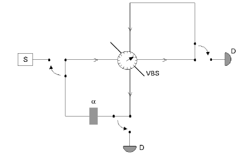
FIG. 1.: A setup that allows two transparencies to be distinguished with an arbitrarily close approximation to the minimum number of absorbed photons, in the case where the two transparencies $\alpha_{1,2}$ are real and have equal a priori probabilities. A single photon source S sends one photon into the apparatus. After the photon has entered, it cycles through the apparatus a certain number of times. In the apparatus the photon first encounters a variable beam splitter (VBS) which sends the photon along two different paths. The object (shaded rectangle), with transparency $\alpha=\alpha_{1}$ or $\alpha_{2}$, is inserted in one of the paths. The initial reflectivity of the VBS is arbitrary but taken to be very small. Thereafter the reflectivity of the VBS changes as described in the text. After having cycled through the apparatus a certain number of times, the photon is sent to one of two detectors depending on which path the photon takes. Note that the photon first passes through the VBS before being sent to the detectors. This ensures that the measurement basis coincides with the path the photon is on. If the detectors do not detect any photon, the experiment is run again until one of the detectors registers a photon. The variable beam splitter and switches used in the setup can be implemented for instance by a Mach-Zehnder interferometer with a variable phase-shifter placed in one of its arms.

Let us analyse the protocol with the formulation used in the proof of the bound. At step $j$ of the protocol, we are in the state

$\displaystyle|\Psi^{j}_{i}\rangle=a^{j}_{i}|1\rangle_{A}|0\rangle_{P}|0\rangle_{O}+b^{j}_{i}|0\rangle_{A}|1\rangle_{P}|0\rangle_{O}+|I^{j}\rangle\ ,$

where $|1\rangle_{A}|0\rangle_{P}|0\rangle_{O}$ corresponds to the photon being present in the empty arm and $|0\rangle_{A}|1\rangle_{P}|0\rangle_{O}$ to the photon being in the object arm, and where $|I^{j}\rangle$ indicates terms where interaction with the object has occurred on previous steps. After the interaction step and the unitary step which acts on $H_{A}\otimes H_{P}$ by the rotation $\left(\matrix{\cos\theta^{j}&-\sin\theta^{j}\cr\sin\theta^{j}&\cos\theta^{j}\cr}\right)$, the state becomes

$$|\Psi_{i}^{j+1}\rangle = (a^{j}_{i}\cos\theta^{j}-\alpha_{i}b^{j}_{i}\sin\theta^{j})|1\rangle_{A}|0\rangle_{P}|0\rangle_{O}$$ (21)

$$\mbox{}+(\alpha_{i}b^{j}_{i}\cos\theta^{j}+a^{j}_{i}\sin\theta^{j})|0\rangle_{A}|1\rangle_{P}|0\rangle_{O}$$

$$\mbox{}+\beta_{i}b^{j}_{i}|0\rangle_{A}|0\rangle_{P}|1\rangle_{O}\}+I^{j},$$

In order to attain our bound we shall examine the different inequalities occurring between steps (7) and (15) and try to saturate them. Note that because there is only one photon present, there are several simplifications. There is only one term under the sum in (7), and thus (8) is an equality. Furthermore, $m=1$ in this term, and for $m=1$ (9) is an equality. So (11) is also an equality. There are two remaining places where an inequality could occur, namely (7) and (13). The first of these will be an equality if

$$\langle\Psi^{j}_{1}|\Psi^{j}_{2}\rangle,\langle\Psi^{j+1}_{1}|\Psi^{j+1}_{2}\rangle$$ (22)

$$\mbox{ and }\langle\Psi^{j}_{1}|\Psi^{j}_{2}\rangle-\langle\Psi^{j+1}_{1}\Psi^{j+1}_{2}\rangle$$ (23)

$$\mbox{ are simultaneously all}\geq 0\mbox{ or }\leq 0,$$ (24)

and the second if $|\beta_{1}C^{j}_{1,km\bf n}|=|\beta_{2}C^{j}_{2,km\bf n}|$, (we are assuming $p_{1}=p_{2}$). For real $\alpha_{i}$, the $a^{j}_{i}$ and $b^{j}_{i}$ will all be real, and the latter condition amounts to

$$\beta_{1}(\alpha_{1}b^{j}_{1}\cos\theta^{j}+a^{j}_{1}\sin\theta^{j}) = \beta_{2}(\alpha_{2}b^{j}_{2}\cos\theta^{j}+a^{j}_{2}\sin\theta^{j}),$$ (25)

or

$$\tan\theta^{j}={{\alpha_{1}\beta_{1}b^{j}_{1}-\alpha_{2}\beta_{2}b^{j}_{2}}\over{\beta_{2}a^{j}_{2}-\beta_{1}a^{j}_{1}}}.$$ (26)

A protocol starts with the initial state $|1\rangle_{A}|0\rangle_{P}|0\rangle_{O}$ so that $b_{1}^{0}=b_{2}^{0}=0$. Thus the angle given by (26) is $\theta^{0}=0$, so no photon ever passes through the object. To avoid this, a first angle of rotation $\theta^{0}\neq$ 0 must be chosen. At the first step, therefore, equality in (13) cannot be achieved. For subsequent steps, however, rotations according to (26) are applied. If $\theta^{0}$ is small, the departure from equality in (13) will be small. However, we can only expect a near approach to our bound, not equality. Note that the condition (25) just says that the probabilities $|\beta_{i}b_{i}^{j+1}|^{2}$ of absorbing a photon are the same for both objects. This means that no information about one of the objects is obtained by the absorption of a photon.

We ran a computational test on our variable angle algorithm (26) to explore its behaviour. The two parameters to choose are the initial angle $\theta^{0}$ and the number of iteration steps $K$. $\theta^{0}$ was chosen randomly (and was taken very small). The maximum number of steps allowed is determined by the condition (24). Since initially $\langle\Psi^{0}_{1}|\Psi^{0}_{2}\rangle=1$ is positive, (24) holds for the first steps until one of the quantities in (24) becomes negative. The smaller the initial angle, the larger the maximum number of steps allowed before (24) is violated. The final state has an overlap $f^{K}=|\langle\Psi_{1}^{K}|\Psi_{2}^{K}\rangle|$, from which the probability of error in distinguishing $|\Psi_{1}^{K}\rangle$ and $|\Psi_{2}^{K}\rangle$ can be computed, using $P_{E}={1\over 2}(1-\sqrt{1-(f^{K})^{2}})$ [10]. The measurement that attains this value of $P_{E}$ is a von Neumann measurement. In order to carry out the measurement one first makes a final unitary transformation and then measures which path the photon takes.

Our strategy is to repeat the protocol until it succeeds (no absorption occurs). Hence the expected number of photons absorbed for object $i$ will be

$$\bar{N}^{abs}_{i} = \sum_{i=1}^{\infty}(1-P(abs|i))P(abs|i)^{n}$$ (27)

$$= P(abs|i)/(1-P(abs|i)).$$ (28)

where $P(abs|i)$ is the probability of absorbing a photon in the protocol.

By varying the value of $K$ in the allowed range, i.e. before (24) is violated, we get a set of algorithms yielding certain values of $P_{E}$. We found that, for all values of $\alpha_{1}$ and $\alpha_{2}$ tested, as the initial angle $\theta^{0}$ was varied, a complete range of values of $P_{E}$ from zero to ${1\over 2}$ was obtained. The small circles in Figures 3 and 4 show this for two values of the $\alpha_{i}$. As can be seen, the bound (solid curve) is closely approached for all the $P_{E}$.

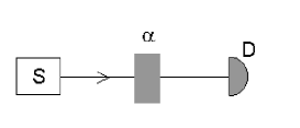
FIG. 2.: A simple classical scheme to distinguish two transparencies. Photons are sent one by one through the object. The number of photons that pass through the object is counted. After each photon is sent, a decision is taken whether it is necessary to continue to send photons through the object, or whether the error probability is sufficiently small.

To compare the quantum bound (1) with classical schemes, figures 3 and 4 also show the mean number of photons absorbed in a photon-counting protocol (illustrated in figure 2). One possible strategy is to send a fixed number of photons through the specimen and decide, by comparing the number absorbed with a predetermined threshold, which object is present. In general, however, fewer photons need be absorbed if the situation is appraised after each photon is transmitted. Suppose that, after the $n$-th photon has been transmitted, $m$ have been absorbed. One calculates the posterior probability $P(1|m,n)=\alpha_{1}^{n-m}\beta_{1}^{m}/(\alpha_{1}^{n-m}\beta_{1}^{m}+\alpha_{2}^{n-m}\beta_{2}^{m})$, assuming still that $p_{1}=p_{2}$, and decides that object 1 is present if $P(1|m,n)>1-x$ and object 2 is present if $P(1|m,n)<x$, where $x$ is a chosen number between 0 and 1/2; otherwise one transmits another photon and repeats the procedure. The number $x$ is therefore the maximum error probability one will tolerate. The actual probability of error with a given $x$ can be calculated empirically by averaging over many trials the values of $P(1|m,n)$ when object 2 is chosen and $1-P(1|m,n)$ when object 1 is chosen. Similarly, the mean number of photons absorbed is obtained by averaging over many trials. Varying $x$ then gives the mean number of absorbed photons as a function of $P_{E}$. As Figures 3 and 4 show, this photon-counting strategy entails a greater expected number of absorbed photons than our algorithm, especially as $P_{E}$ tends to zero (when the number of photons absorbed by the counting strategy must tend to infinity). For instance, for $P_{E}=0.01$, only $75\%$ of the classical light is needed for $\alpha_{1}=0.2$, $\alpha_{2}=0.3$ and $63\%$ for $\alpha_{1}=0.2$, $\alpha_{2}=0.8$.

FIG. 3.: The average number of photons absorbed, $\bar{N}^{abs}$, for a given error probability $P_{E}$, for $\alpha_{1}=0.2$, $\alpha_{2}=0.3$. Each circle represents a protocol given by (26), with a particular random choice of initial angle. Protocols were selected by the condition that $\bar{N}^{abs}$ differed by less than $10^{-4}$ from the bound of (1). The diamonds represent numbers of photons absorbed with the photon counting protocol described in the text. Note how the curves diverge for $P_{E}\to 0$, since a quantum protocol can distinguish with certainty between two transparencies with a finite number of absorbed photons whereas a classical absorption protocol requires an infinite number of absorbed photons for perfect discrimination.

FIG. 4.: The average number of photons absorbed, as a function of $P_{E}$, for $\alpha_{1}=0.2$, $\alpha_{2}=0.8$. Notation as in Figure 1. Note that for the photon counting protocol described in the text the error probability $P_{E}$ can only take discrete values. For instance for the values of $\alpha_{1,2}$ chosen here, if no photons are sent through the object, $P_{E}=0.5$ and if a single photon is sent through the object $P_{E}=0.2$. Smaller values of $P_{E}$ require more photons.

In conclusion, for a given probability of error, the mean number of absorbed photons given by our quantum bound eq. (1) is less than that expected from a simple absorption technique. The bound we have derived is valid for any quantum protocol, using any number of photons, ancillae, etc. However, we have shown that, for real transparencies and equal prior probabilities, a single photon protocol can approch our bound arbitrary closely. This suggest that using many photons or coherent light is not as good as using a single photon source. It would be interesting to know whether similar types of protocols allow our bound to be saturated in the case of complex transparencies and unequal prior probabilities. The latter case deserves particular attention, since the advantage of our bound over the classical limits seems to be most marked for unequal priors.

REFERENCES

• [1] Elitzur, A. C. and Vaidman, L., Found. of Phys.23, 987-997 (1993).
• [2] Kwiat, P., Physica Scripta T76, 115 (1998).
• [3] Jang, J.-S., Phys. Rev. A, 59, 2322-2329 (1999).
• [4] Krenn, G., Summhammer, J. and K. Svozil, Phys. Rev. A 61, 052102 (2000)
• [5] Mitchison, G. and Massar, S., Phys, Rev. A 63 (2001), 032105
• [6] Massar, S., Mitchison, G. and Pironio, S. preprint available at http://xxx.lanl.gov/quant-ph/0102116.
• [7] Kent, A. and Wallace, D., preprint available at http://xxx.lanl.gov/quant-ph/0102118.
• [8] P. Facchi, Z. Hradil, G. Krenn, S. Pascazio, J. ŘehÑčk, preprint available at http://xxx.lanl.gov/quant-ph/0104021.
• [9] Kwiat, P. G., Weinfurter, H., Herzog, T., Zeilinger, A. and Kasevich, M. A., Phys. Rev. Lett. 74, 4763-4766 (1995).
• [10] C. W. Helstrom, Quantum Detection and Estimation Theory, (Academic Press, New York,1976)