The -function-kicked rotor: Momentum diffusion and the quantum-classical boundary
LA-UR-01-1909
Abstract
We investigate the quantum-classical transition in the delta-kicked rotor and the attainment of the classical limit in terms of measurement-induced state-localization. It is possible to study the transition by fixing the environmentally induced disturbance at a sufficiently small value, and examining the dynamics as the system is made more macroscopic. When the system action is relatively small, the dynamics is quantum mechanical and when the system action is sufficiently large there is a transition to classical behavior. The dynamics of the rotor in the region of transition, characterized by the late-time momentum diffusion coefficient, can be strikingly different from both the purely quantum and classical results. Remarkably, the early time diffusive behavior of the quantum system, even when different from its classical counterpart, is stabilized by the continuous measurement process. This shows that such measurements can succeed in extracting essentially quantum effects. The transition regime studied in this paper is accessible in ongoing experiments.
pacs:
03.65.Bz,05.45.Ac,05.45.PqI Introduction
Explorations of the transition from quantum to classical behavior in nonlinear dynamical systems constitute one of the frontier areas of present theoretical research. The recently realized possibility of carrying out controlled experiments in this regime exp1 ; exp2 ; exp3 has added greatly to the impetus for increasing our understanding of this transition, quite aside from the undoubtedly fundamental importance of the subject. The point at issue is not so much the status of formal semiclassical approximations in the sense of taking the mathematical limit , but a description and understanding of the processes that take place in actual experiments on the dynamical behavior of observed quantum systems. Quantum decoherence and conditioned evolution arising as a consequence of system-environment couplings and the act of observation provide a natural pathway to the classical limit as has been demonstrated quantitatively in Ref. bhj (see also references clmeas1 ) and is reviewed in the next section.
Comparison of the dynamics of closed quantum and classical systems in explicit examples has shown a variety of behaviors. At the one extreme, there exist systems where quantum and classical averages track each other for long times long , and at the other extreme, there are systems in which the averages break away from each other decisively at finite times short . Since even this second class of systems do attain classical dynamics when the action is sufficiently large, they undergo a clear transition from a ‘quantum’ to a ‘classical’ behavior as the parameters of the system controlling its action are varied, and are of particular interest to a study of the quantum-classical transition. The quantum delta-kicked rotor (QDKR) is a well-studied example of this class of system and it is our purpose here to investigate the quantum-classical transition in this system within the framework based on the theory of continuous measurement presented in Ref. bhj . As will be demonstrated below, the quantum-classical transition regime possesses some remarkable features which are well within the reach of present-day experiments.
One of the remarkable features of the QDKR which distinguishes it from its classical counterpart is the behavior of its late time momentum diffusion constant, . In the classical case, this quantity attains a constant value, , whereas for the QDKR, it falls to zero. This latter phenomenon is termed dynamical localization dloc . In addition, the QDKR also displays a nontrivial variation of the early-time intrinsic momentum diffusion coefficient, , as a function of the stochasticity parameter shep , and strong resistance to decoherence qdkrdeco ; cohen ; hjmrss ; milner ; steck ; scalings . This last feature relates to the fact that it is possible for external noise and decoherence to break dynamical localization in the sense that the late-time quantity , nevertheless remains small and far from its classical value unless very strong noise strength is employed. Finally, the QDKR possesses the added attraction that it can be studied via atomic optics experiments utilizing laser-cooled atoms and allowing some degree of control of the coupling to an external environment via spontaneous emission processes exp2 . This system consists of noninteracting atoms in a magneto-optical trap (MOT); on turning on a detuned standing light wave with wave number , the atoms scatter photons resulting in an atomic momentum kick of with every such event. Internal degrees of freedom can be eliminated since the large detuning precludes population transfer between atomic states. The resulting dynamics is restricted to the momentum space of the atoms and can be described by simple effective Hamiltonians, the Hamiltonian for the QDKR being one of the implementable examples.
Our main consideration is a systematic analysis of the quantum-classical transition induced via position measurement for the non-dissipative delta-kicked rotor using the late-time momentum diffusion rate as a diagnostic tool. Even though quantum dynamical localization typically suppress late time diffusion ( at late times), we find that a small measurement strength (i.e., weak noise) can stabilize an intrinsically quantum early time effect (the enhancement of the initial quantum diffusion rate predicted by Shepelyansky shepscaling ) and produce a nonzero final diffusion rate much larger than the classical value. The predicted effect is large and should be observable in present experiments studying the quantum-classical transition in the QDKR. We also comment on the behavior of the diffusion coefficient near a quantum resonance and on the nontrivial nature of the approach to the classical noise-dominated value for the diffusion rate as the noise induced by the measurement is increased. Our theoretical results have been confirmed recently by a more detailed analysis relevant to specific experimental realizations nz .
The plan of the paper is as follows. In Section II, we provide a short review of recent work on continuous measurement and the quantum-classical transition, moving on to the specific case of the QDKR in Section III. In Section IV, we explain how the late-time diffusion coefficient provides a window to investigate the quantum-classical transition in this system and in Section V we describe the detailed nature of the transition. Section VI is a short conclusion.
II Continuous Measurement and the Quantum to Classical Transition
Macroscopic mechanical systems are observed to obey classical mechanics. However, the atoms which ultimately make up the macroscopic systems certainly obey quantum mechanics. Since classical and quantum evolution are different, the question of how the observed classical mechanics emerges from the underlying quantum mechanics arises immediately. This emergence, referred to as the quantum to classical transition, is particularly curious in the light of the fact that classical mechanical trajectories are governed by nonlinear dynamics that often exhibit chaos, whereas the very concept of a phase space trajectory for a closed quantum system is ill-defined, and any signatures of chaos are, at best, indirect.
If quantum mechanics is really the fundamental theory, then one must be able to predict the emergence of (the often chaotic) classical trajectories by describing a macroscopic object with sufficient realism, but fully quantum mechanically. Sufficient ingredients to perform such a description have now been found bhj ; clmeas1 . The solution has involved the realization that all real systems are subject to interaction with their environment. This interaction does at least two things. First, it subjects the system to noise and damping CL ; qnoise (as a consequence all real classical systems are subject to noise and damping - even if very small), and second, the environment provides a means by which information about the system can be extracted (effectively continuously if desired), providing a measurement of the system cm .
Since observation of a system is essential in order that the trajectories followed by that system can be obtained and analyzed (this being just as true classically as quantum mechanically), it may be expected that this process must be included in the description of the macroscopic system in order to correctly predict the emergence of classical trajectories. An example of an environment that naturally provides a measurement is that of the (quantum) electromagnetic field with which the system is surrounded. Monitoring this environment consists of focusing the light which is reflected from the system, allowing the motion to be observed. If the environment is not being monitored, then the evolution is simply given by averaging over all the possible motions of the system. (Classically this means an average over any uncertainty in the initial conditions, and over the noise realizations.)
It has now been established quantitatively that continuous observation of the position of a single quantum mechanical degree of freedom, is sufficient to correctly predict the emergence of classical motion when the action of the system is sufficiently large compared to . In particular, inequalities have been derived involving the strength of the environmental interaction and the Hamiltonian of the system, which, if satisfied, will result in classical motion bhj (see also clmeas1 ). These inequalities, therefore, refine the notion of what it means for a system to be macroscopic.
A detailed explanation of the reason that continuous measurement induces the qantum-to-classical transition may be found in Refs. bhj ; bhj2 ; bhjLA . To recapitulate that analysis, the emergence of classical behavior arises from simultaneous satisfaction of two counteracting constraints. The first is that a sufficiently strong observation process is needed to maintain localization of the particle in phase space, and, thereby, produce classical motion of the centroid of the Wigner function bhj from Ehrenfest’s theorem. On the other hand, even for a localized distribution, a strong measurement introduces noise into the system, and this needs to be bounded to a microscopic scale. These constraints are satisfied for an ever increasing range of measurement strengths as the system parameters become large enough to make the quantum unit of action, i.e., , negligible. Thus, when systems are sufficiently macroscopic, they exhibit classical motion with a negligible amount of irreducible quantum noise, a noise that, in practice, is always swamped by classical measurement uncertainties and tiny environmental disturbances.
As mentioned above, these arguments can be codified into a set of inequalities. First, to maintain enough localization to guarantee that, at a typical point on the trajectory, one has for the force , , as required in the classical limit, the measurement strength (defined precisely in the next section), , must stop the spread of the wavefunction at the unstable points footnote1 , :
| (1) |
Second, as noted already, a large measurement strength introduces noise into the trajectory. Demanding that averaged over a characteristic time period of the system, the change in position and momentum due to the noise are small compared to those induced by the classical dynamics, it is sufficient that, at a typical point on the trajectory, the measurement satisfy
| (2) |
where is the typical value of the action footnote2 of the system in units of and ranges from zero to unity and characterizes the efficiency of the measurement (for the measurements considered in this paper, ). Obviously as becomes large, this relationship is satisfied for an ever larger range of , and this defines the classical limit.
This understanding of the quantum-to-classical transition in terms of quantum measurement which has emerged within the last ten years is, of course, completely consistent with the mechanism usually referred to as decoherence, since averaging over the results of the measurement process gives the same evolution as an interaction with an unobserved environment (in particular, the environment through which the system is being monitored) in which the environment is traced over. Thus, the treatment in terms of measurement is actually a microscopic analysis of the process of decoherence. However, examining the measurement process allows us to obtain an understanding of why it is that decoherence causes classical motion to emerge, and also allows us to realize the trajectories themselves, something that is impossible when the environment is merely traced over. The knowledge of the dynamics of the individual quantum trajectories provides new information not available from a traditional decoherence analysis and, as we show below, this more microscopic information can be helpful in understanding phenomena even at the level of expectation values.
With this understanding of the mechanism of the emergence of classical motion, it becomes pertinent to ask the question, how does the dynamics of a particular system change as it is made more macroscopic? That is, what happens to the dynamics as it passes through the transition from quantum motion (when its action is very small), to classical motion (when its action is sufficiently large). In the following sections we address this question for the delta-kicked rotor.
III QDKR Under Continuous Observation
The Hamiltonian controlling the evolution of the QDKR is
| (3) |
It is more convenient to study this system by rescaling variables, in terms of which the new Hamiltonian becomes scalings
| (4) |
where and are dimensionless position and momentum, satisfying , for a dimensionless , and is the scaled kick strength. Following the experimental situation, we will use a typical value of and open boundary conditions on . The value of is a measure of the system action relative to . When is small, the system action is large compared to and the system can be considered to be effectively macroscopic. Conversely, when is large, the system is microscopic and will behave quantum mechanically under weak environmental interaction. The ability to change the system action relative to (i.e., changing ) allows a systematic experimental study of the quantum-classical transition. The parameter ranges we have studied numerically below have been chosen to be more or less typical of those utilized in present experiments. Finally, we note that the scaling required to bring the equation to this dimensionless form hides the fact that increasing the dimensionless effective Planck’s constant at fixed involves increasing the period between the kicks and decreasing their strength — thus, all else being equal, this system is expected to behave more clasically under observation when the kicks are harder and spaced closer in time.
The effect of random momentum kicks due to spontaneous emission can be modeled approximately by a weak coupling to a thermal bath spontem . In current experiments the atom interacts with a standing wave of laser light leading to a (sinusoidal) spatial modulation of the bath coupling. This modulation in turn produces a corresponding spatial variation in the diffusion coefficient of the Master equation describing the evolution of the reduced density matrix for the position of the atom. In the language of continuous measurements, spontaneous emission can be regarded as a measurement of a function of the position , namely . While one can certainly study this class of measurement processes, in this paper we will study the case of continuous measurements of position. In general, as far as the study of the quantum-classical transition is concerned, the exact nature of the measurement process is not expected to be important provided that it yields sufficient information to enable the observer to localize the system in phase space.
A continuous measurement of position is described by the (nonlinear) stochastic Schrödinger equation sse
| (5) | |||||
where the continuous measurement record obtained by the observer is
| (6) |
being Wiener noise. The noise represents the inherent randomness in the outcomes of measurements. Aside from the unitary evolution, this equation describes changes in the system wave function as a result of measurements made by the observer. The parameter characterizes the rate at which information is extracted from the system djj .
Averaging over all possible results of measurements leads to a Master equation describing the evolution of the reduced density matrix for the system. This Master equation has the form
| (7) |
where the diffusion coefficient is given by , with the diffusion constant describing the rate at which the momentum of a free particle would diffuse due to a thermal environment. From the relationship between and given above, we see that determines the relationship between the information provided about , and the resulting momentum disturbance. The important point to note for the following is that for a fixed , the measurement strength is reduced as increases (conversely, for fixed measurement strength increases with ). The stochastic Schrödinger equation (5) is said to represent an unraveling of the Master equation (7) with averages over the Schrödinger trajectories reproducing the expectation values computed using the reduced density matrix .
All dynamical systems that one can build in the laboratory are necessarily observed in order to investigate their motion. For sufficiently small , and a reasonable value of , the measurement maintains localization of the wavefunction, while generating an insignificant . For sufficiently localized wavefunctions, expectation values of products of operators are very close to the products of the expectation values of the individual operators. Ehrenfest’s theorem then implies that the classical equations of motion are satisfied. On the other hand, for sufficiently large (and the same insignificant ), is sufficiently small that the quantum dynamics is essentially preserved. It is the detailed nature of this transition that we now wish to investigate.
IV Quantum-Classical Transition and the Late-Time Diffusion Coefficient
Our strategy in examining the quantum to classical transition is to fix the level of noise (i.e., the diffusion coefficient ) resulting from the measurement at some sufficiently small value, so that classical behavior is obtained for small and then to study systematically how quantum behavior emerges as is increased. The key diagnostic is the behavior in time of the expectation value of momentum squared, . Previous studies of the QDKR have shown that in the presence of decoherence/measurement, dynamical localization is lost in the sense that there exists a non-zero late-time momentum diffusion coefficient, but that this diffusion coefficient is not necessarily the same as the intrinsic classical diffusion coefficient qdkrdeco ; cohen . The existence of this late-time diffusion coefficient provides a particularly convenient means of characterizing and studying the quantum-classical transition: The late-time diffusion coefficient is an unambiguous, theoretically well-defined quantity and, moreover, is also measurable in present experiments.
In the classical regime (when is sufficiently small), attains the classical value () with . This should not be confused with the noisy classical limit which arises under strong driving by the noise (large ) in which case rrw . At sufficiently large values of , on the other hand, one expects quantum effects to be dominant and therefore one should very nearly obtain dynamical localization (). Thus, one of the key questions is the behavior of as a function of in the transition regime in between and , and the variation of as a function of decoherence or measurement strength as set by the value of .
Analytical investigation of the transition regime is made difficult by the nonlinearity of the dynamical equations and the lack of a small parameter in which to carry out a perturbative analysis fnote . The nonlinearity results from the fact that the measurement record drives the evolution of the wave function in equation (5) and, at the same time, is itself dependent on the expectation value of the position. We solved the nonlinear Schrödinger equations (5) numerically.
Numerical investigation of the dynamics of the environmentally coupled QDKR requires the solution of a stochastic, nonlinear partial differential equation. In order to obtain the desired ensemble averages, one needs to average over many noise realizations for each set of parameters considered. We implemented a split-operator spectral algorithm on a parallel supercomputer to solve Eq. (5), and then averaged over the resulting trajectories to obtain the solution to Eq. (7). (Direct solution of Eq. (7) to the desired accuracy is still a major challenge for supercomputers.) Grid sizes for computing the wave function ranged from depending on the value of and . One thousand realizations were averaged over for each data point. Our numerical results for the transition regime contain a variety of interesting phenomena which we discuss below.
V The Structure of the Quantum-Classical Transition
The generic behavior of quantum trajectories is the following. If we construct a trajectory starting with a minimum uncertainty wavepacket, the nonlinearity of the system dynamics tends to spread it out. However, the localizing influence of measurement limits the spread (in both and ), and a steady state is eventually attained. The stronger the measurement, the sooner the spread is checked. This behavior of individual trajectories appears to be the key to understanding even though, in this case, we are interested not in single trajectories, but in the behavior of an ensemble of these trajectories.
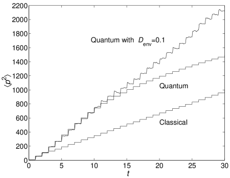
In Fig. 1 we plot for the classical system, and for the quantum system with and without measurement for . (Using the results of bhj , classical behavior is not expected unless and .) At early times, the quantum value of the diffusion rate is much higher than the classical value, although, consistent with dynamical localization, this decreases with time (eventually falling to zero). On the other hand, when the system is under observation, the initial evolution of the system is hardly affected; it is only that the diffusion rate reaches a constant value at about (for this value of ) at which point a purely diffusive evolution takes over. Thus, the measurement appears to induce a ‘premature’ (time-dependent) steady-state, just as it induces a ‘premature’ steady-state width bhj . Thus the diffusion rate gets frozen in to its early time value which, in this case, is substantially larger than the classical result.
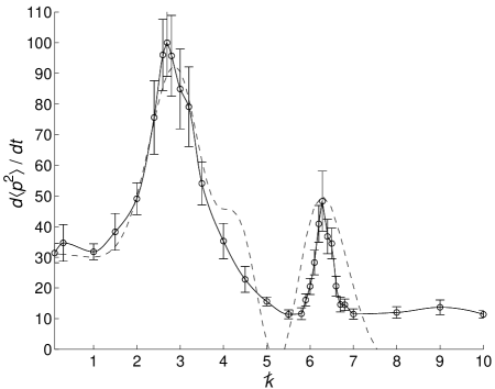
In Fig. 2 we plot as a function of for and , with . For small , is essentially given by the classical value (), and for large , is close to the quantum value () when is sufficiently small. Thus we see the expected transition from classical to quantum behavior. However, the transition region is surprisingly complex: the value of in this region varies widely as a function of and rises to more than twice at its peak! Another remarkable fact is that features and placement of the transition region (as a function of ) is relative insensitive to the value of as it changes over three orders in magnitude. In what follows, for convenience we will refer to the plots in Fig. 2 simply as transition curves.
Some understanding of this complex structure can be obtained by comparison with the early time diffusion rate for the unmeasured quantum system as derived analytically by Shepelyansky,
| (8) |
where . This approximate expression for is also plotted in Fig. 2. As this formula is only valid for , a condition not met over most of this range, we use it only as a qualitative indicator (it is a particularly poor indicator of the actual behavior near the quantum resonance at ). Nevertheless, the trend in the data is obvious: we see that for sufficiently large , the transition curve follows the early time quantum diffusion rate fairly closely over the region of the first peak: measurement is effective at ‘freezing in’ the early time value, and it is from this that the complex structure originates.
The structures in the transition region can therefore be qualitatively understood in terms of this expression. Comparison of Eq. 8 with an expression shepscaling for shows that this initial diffusion rate in units of the square of the kick strength, , are identical except for a renormalization of to . The classical system, however, possesses regimes of increased diffusion due to the presence of accelerator modes at certain values of . In the quantum system, we can scan through these values of by tuning , provided is large enough. This is the origin of the first peak in the transition region for our value of : at , , which is the position of the first such accelerator mode.
The scaled classical diffusion constant, , also increases as . This leads to an interesting behaviour in the quantum expression because by choosing , we can tune even when remains non-zero. Correspondingly the quantum system with this value of shows an enhanced early diffusion which has no simple classical counterpart. In fact, in a purely quantum mechanical approach, this very narrow quantum resonance steck arises due to quantum mechanical interference effects with no classical analog. It is remarkable that these inherently quantum mechanical effects survive and, in fact, are stabilized by continuous measurement and the associated decoherence in the Master equation (7). This counter-intuitive behavior results in part from the fact that the QDKR strongly resists decoherence to classicality as explained in Ref. hjmrss .
For smaller values of , the transition curve drops below the Shepelyansky predictions for the diffusion rate, which is consistent with the notion that the weaker measurement takes longer to stabilize the falling quantum diffusion rate. As is evident from Fig. (1) locking in at a later time on the noiseless quantum curve will clearly produce a smaller value of the diffusion coefficient.

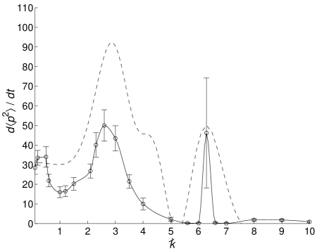
One consequence of this complex behavior is that, in the transition region, the cross-over from the classical to quantum regimes can also lead to effects that are quite counter-intuitive. An example of such behavior is exposed by plotting the late-time as a function of for different values of as we have done in Fig. 3. One interesting open question that can be addressed this way is whether the quantum evolution, as a function of , first goes over to the classical limit (with small noise) or reaches the classical value only in the fully noise dominated limit. At sufficiently small and a finite , it follows from the results of Ref. bhj that the classical limit will exist and thus the quantum evolution will go over to the small-noise classical limit. However, as Fig. 3 shows, in the intermediate regime this is not the case. Indeed, for a range of values of , an inversion of what is usually expected occurs: The system diffuses slower (intuitively, a ‘more quantum’ behavior) at smaller values of (e.g., vs. in Fig. 3).
In summary, we would like to emphasize certain important points regarding the transition curve. The first is that examining only the transition curve, one might conclude that the classical limit has been achieved when the classical value of has been reached (e.g. at for ), especially since it remains at this value for smaller . However, examining the position probability distribution of the particle for a typical trajectory with , and , we find that far from being well localized, the particle position is spread significantly over four periods of the potential, and the distribution contains a great deal of complex structure. As a result, the individual trajectories, which are in principle measurable, are still far from classical fnote2 . Evolving for small reveals that true classical motion emerges at the trajectory level for only when , as expected from the conditions in Ref. bhj . The second point is that since the transition curves rise above the classical value in the intermediate regime, they necessarily cross this value again during their descent into the quantum region. Hence it is important not to sample the curve only in a limited region, in which case one could mistakenly conclude that the transition from quantum to classical behavior of the diffusion constant had already taken place.
Experimental verification of our predictions should be within reach of the present state of the art. Either spontaneous emission or continuous driving with noise should be, in principle, sufficient to observe the anticipated diffusive behavior in (see, e.g., Ref. scalings ). Measuring accurately can, however, still be complicated by problems with spurious tails in the momentum distribution, nevertheless, these problems can likely be overcome especially since the predicted effects do not require the experiments to be run for long times (see Ref. darcy for a recent measurement of the behavior near the quantum resonances including decoherence effects).
VI Conclusion
To conclude, we reemphasize a few key points: We have shown that it is possible to characterize the quantum-classical transition in the QDKR by fixing the environmentally induced diffusion () at some sufficiently small value, and examining the late-time diffusion coefficient as the size of the system is increased ( decreased). In doing so, we have shown that the late-time behavior in the transition region is strikingly complex and different from both the classical and quantum behavior, and that this dynamics follows, instead, the early time quantum diffusion rates. Remarkably, the temporary nature of the early-time quantum diffusion rates is in fact stabilized by the continuous measurement allowing for their possible measurement. These predictions for a distinct, experimentally accessible, ‘transition dynamics’ provide an interesting area for investigation in experiments currently being performed on the quantum delta-kicked rotor.
VII Acknowledgements
We thank Doron Cohen, Andrew Daley, Andrew Doherty, Scott Parkins, Daniel Steck, and Bala Sundaram for helpful and stimulating discussions. K.J. would like to thank Scott Parkins for hospitality at the University of Auckland during the development of this work. Numerical calculations were performed at the Advanced Computing Laboratory, Los Alamos National Laboratory, and at the National Energy Research Scientific Computing Center, Lawrence Berkeley National Laboratory.
References
- (1) M. Brune, E. Hagley, J. Dreyer, X. Maitre, A. Maali, C. Wunderlich, J.M. Raimond, and S. Haroche, Phys. Rev. Lett. 77, 4887 (1996); C.J. Hood, T.W. Lynn, A.C. Doherty, A.S. Parkins, and H.J. Kimble, Science 287, 1447 (2000).
- (2) H. Ammann, R. Gray, I. Shvarchuck, and N. Christensen, Phys. Rev. Lett. 80, 4111 (1998); B.G. Klappauf, W.H. Oskay, D.A. Steck, and M.G. Raizen, ibid 81, 1203 (1998).
- (3) D.L. Haycock, P.M. Alsing, I.H. Deutsch, J. Grondalski, and P.S. Jessen, Phys. Rev. Lett. 85, 3365 (2000).
- (4) T. Bhattacharya, S. Habib, and K. Jacobs, Phys. Rev. Lett. 85, 4852 (2000).
- (5) T.P. Spiller and J.F. Ralph, Phys. Lett. A 194, 235 (1994); M. Schlautmann and R. Graham, Phys. Rev. E 52, 340 (1995); R. Schack, T.A. Brun, I.C. Percival, J. Phys. A 28, 5401 (1995); T.A. Brun, I.C. Percival, and R. Schack, J. Phys. A 29, 2077 (1996); I.C. Percival and W.T. Strunz, J. Phys. A, 31, 1815 (1998); J. Phys. A, 31, 1801 (1998); A.J. Scott and G.J. Milburn, Phys. Rev. A 63, 042101 (2001).
- (6) L.E. Ballentine, Y. Yang, and J.P. Zibin, Phys. Rev. A 50, 2854 (1994); B.S. Helmkamp and D.A. Browne, Phys. Rev. E 49, 1831 (1994); R.F. Fox and T.C. Elston, ibid. 49, 3683 (1994); ibid. 50, 2553 (1994).
- (7) G. Casati, B.V. Chirikov, F.M. Izrailev, and J. Ford, in Stochastic Behavior in Classical and Quantum Hamiltonian Systems, edited by G. Casati and J. Ford, Lecture Notes in Physics Vol. 93 (Springer, New York, 1979); F. Haake, M. Kus and R. Scharf, Z. Phys. B 65, 381 (1987).
- (8) G. Casati et al. cited in Ref. short .
- (9) A.B. Rechester and R.B. White, Phys. Rev. Lett. 44, 1586 (1980).
- (10) E. Ott, T.M. Antonsen, and J.D. Hanson, Phys. Rev. Lett. 53, 2187 (1984); T. Dittrich and R. Graham, Z. Phys. B 62, 515 (1986); Europhys. Lett. 7, 287 (1988); Ann. Phys. 200 363 (1990); Phys. Rev. A 42, 4647 (1990); M. Schlautmann and R. Graham, in Ref. clmeas1 above; S. Dyrting and G.J. Milburn, Quantum and Semiclassical Optics 8, 541 (1996).
- (11) D. Cohen, Phys. Rev. A 44, 2292 (1991).
- (12) S. Habib, K. Jacobs, H. Mabuchi, R.D. Ryne, K. Shizume, and B. Sundaram, Phys. Rev. Lett. (submitted), quant-ph/0010093.
- (13) V. Milner, D.A. Steck, W.H. Oskay, and M.G. Raizen, Phys. Rev. E 61, 7223 (2000).
- (14) W.H. Oskay, D.A. Steck, V. Milner, B.G. Klappauf and M.G. Raizen, Opt. Comm. 179, 137 (2000).
- (15) D.A. Steck, V. Milner, W.H. Oskay, and M.G. Raizen, Phys. Rev. E, 62, 3461 (2000).
- (16) D.L. Shepelyansky, Physica D 28, 103 (1987).
- (17) A.J. Daley, A.S. Parkins, R. Leonhardt, and S.M. Tan, quant-ph/0108003.
- (18) See, e.g., A.O. Caldeira and A.J. Leggett, Ann. Phys. (N.Y.) 149, 374 (1983); Physica A 121, 587 (1983).
- (19) C.W. Gardiner and P. Zoller, Quantum Noise, 2nd edition (Springer, Berlin, 2000).
- (20) Early work includes A. Barchielli, L. Lanz, and G.M. Prosperi, Nuovo Cimento 72B, 79 (1982); N. Gisin, Phys. Rev. Lett. 52, 1657 (1984); L. Diosi, Phys. Lett. A 114, 451 (1986); C.M. Caves and G.J. Milburn, Phys. Rev. A 36, 5543 (1987); V.P. Belavkin, Nondemolition measurements, nonlinear filtering and dynamic programming of non-linear stochastic processes, Lect. Notes in Control and Information Sciences 121, (Springer, Berlin, 1988); H. Carmichael, An Open Systems Approach to Quantum Optics (Springer, Berlin, 1993); H.M. Wiseman and G.J. Milburn, Phys. Rev. A 47, 642 (1993).
- (21) T. Bhattacharya, S. Habib, and K. Jacobs (in preparation).
- (22) T. Bhattacharya, S. Habib, and K. Jacobs, Los Alamos Science (in press).
- (23) Actually, if the nonlinearity is large on the quantum scale, , needs to be much larger than , irrespective of the sign of . This does not change the argument in the body of the paper.
- (24) We are assuming that both and evaluated at a typical point of the trajectory are comparable to the action of the system, and define this to be .
- (25) S. Dyrting, Phys. Rev. A 53, 2522 (1996).
- (26) V.P. Belavkin and P. Staszewski, Phys. Lett. A 40, 359 (1989).
- (27) A.C. Doherty, K. Jacobs, and G. Jungman, Phys. Rev. A 63, 062306 (2001).
- (28) C.F.F. Karney, A.B. Rechester, and R.B. White, Physica D 4, 425 (1982).
- (29) Approximate analytic results for a related model have been derived by Cohen cohen . However, these are not directly applicable to the case considered here.
- (30) It is unknown whether or not the non-classicality of the trajectories leaves a signature detectable in ensemble measurements.
- (31) M.B. d’Arcy, R.M. Godun, M.K. Oberthaler, D. Cassettari, and G.S. Summy, Phys. Rev. Lett. 87, 074102 (2001).