Monte Carlo Simulation of Laser Diodes Sub-Poissonian Light Generation

When laser diodes are driven by high-impedance electrical sources the variance of the number of photo-detection events counted over large time durations is less than the average number of events (sub-Poissonian light). The paper presents a Monte Carlo simulation that keeps track of each level occupancy (0 or 1) in the conduction and valence bands, and of the number of light quanta in the optical cavity. When there is good electron-lattice thermal contact the electron and hole temperatures remain equal to that of the lattice. In that case, elementary laser-diode noise theory results are accurately reproduced by the simulation. But when the thermal contact is poor (or, almost equivalently, at high power levels) new effects occur (spectral-hole burning, temperature fluctuations, statistical fluctuations of the optical gain) that are difficult to handle theoretically. Our numerical simulation shows that the frequency domain over which the photo-current spectral density is below the shot-noise level becomes narrower as the optical power increases.

1 Introduction

Light is called sub-Poissonian when the variance of the number of photo-detection events counted over a large time duration is less than the average number of events. Equivalently, we may say that the photo-current spectral density is below the shot-noise level at low Fourier (or baseband) frequencies. It has been shown experimentally in 1987 [1] that laser diodes driven by high-resistance electrical sources may generate sub-Poissonian light. This feature of great fundamental and practical importance treated theoretically in [1] on the basis of the laws of Quantum Optics may be understood alternatively as resulting from a birth-death Markov process [2, 3]. Such processes, as they apply to lasers in general, were discussed in particular by Jakeman and Loudon [4, 5]. The reader will find a clear mathematical discussion in [6].

The originality of the present simulation rests on the fact that electronic level occupancies and light quanta are accounted for individually, the photo-detection rate being derived from a Monte Carlo simulation of the system evolution in the course of time. All microscopic physical processes are (or could be) accounted for. Electron level occupancies (0 or 1) fluctuate as a result of internal electronic transitions (Auger transitions, thermalization and interaction with the optical field stored in the laser cavity), pumping and optical absorption.

An exhaustive Monte Carlo simulation has apparently not been reported before, probably because of the high computer time required in the case of bulk semiconductor lasers. But dramatic size reductions have been obtained with microcavity quantum dot lasers [7] and two-dimensional photonic-bandgap quantum-dots lasers [8]. Because the active layers involve few optically active quantum dots in the gain region an individual account of each level occupancy is manageable. Such devices, likely to be the next generation semiconductor lasers provided technological problems are overcome to achieve efficient electrical pumping, may be labeled ‘mesoscopic’ because of their small size. Note that in optical computing applications only small optical output powers are needed and small driving currents are desired.

For conventional applications, e.g., optical communications, milliwatts of powers are usually required. In that case, our simulation results have to be scaled up since it would be impractical to account for every level occupancy in the case of bulk semiconductors. Scaling laws applicable to the linearized theory need generalization if one wishes to take into account advanced effects such as spectral-hole burning. Our numerical results help ascertain the validity of advanced theories.

The main processes involved in laser light generation are recalled in Section 2, and the numerical procedure is explained in Section 3. Numerical results concerning photodetection noise are illustrated in Section 4 and the conclusion in Section 5. The analytical formula in the appendix derives from the birth-death process through linearization and the assumption that the Fermi-Dirac distribution at some constant temperature $T$ adequately describes electronic level occupancies. An explicit expression of the photo-detection spectrum is obtained for evenly-spaced electronic levels (spacing $\epsilon$) and a non-fluctuating electron injection rate $J$. It is shown that the photo-detection spectrum depends only on the light absorption constant $\alpha$ and the normalized pumping rate $J^{\star}\equiv J\epsilon/k_{B}T$.

2 Laser Diode Processes

In the present section the basic Physics of semiconductors, and processes relevant to isolated cavities containing semiconductors in contact with a thermal bath, are first recalled. Pumping and optical absorption are discussed subsequently.

One-electron energy levels in the semiconductor are supposed to be of the form $\epsilon_{k}=k\epsilon$, with $k$ an integer and $\epsilon$ a constant. The lasers considered may incorporate quantum dots in the gain region. The evenly-spaced-level assumption is then justified by the mechanism of level ‘repulsion’ observed in nanometer-scale irregular particles [9]: the probability that adjacent levels be separated by $\epsilon$ is of the form $\epsilon^{4}\exp(-\epsilon^{2})$, a sharply peaked function of $\epsilon$. Note also that quantum wells exhibit levels that are evenly spaced on the average within each sub-bands. That is, the density of states is a constant.

Some levels are allowed while others are forbidden. Allowed levels may be occupied by at most one electron to comply with the Pauli exclusion principle. The electron spin, ignored in the present paper for the sake of brevity, is discussed for example in [10]. Our model considers neither electronic superposition states nor any strong Coulomb interaction, approximations made in virtually all laser-diode theories. In semiconductors the allowed electronic levels group into two bands, the upper one being called conduction band (CB) and the lower one valence band (VB). We suppose that both bands involve the same number $B=100$ of levels, and are separated by $G_{p}$ forbidden levels as shown in Fig. 1. The band gap energy $G_{p}\epsilon$ is instrumental in determining the laser oscillation frequency but it will not enter in our model because of simplifying assumptions to be later discussed. Only one valence band is considered, but it would be straightforward to take into account the heavy-hole, light-hole and split-off bands found in most semiconductors. $N=B$ electrons are allocated to the allowed energy levels. For pure semiconductors at $T=0$ K, the $N$ electrons fill up the valence band while the conduction band is empty. The electron-lattice system is electrically neutral.

Without a thermal bath, the electron gas reaches an equilibrium state through Auger-type transitions: an electron gets promoted to upper levels while another electron gets demoted to lower levels in such a way that the total energy remains the same. The two electrons may belong to the same band or to distinct bands, but only the former situation is presently considered. Auger transitions ensure that all the system microstates are being explored in the course of time so that electron gases possess well-defined temperatures at any instant in each band. Nothing, however, prevents these temperatures from fluctuating in the course of time. The Coulomb interactions on which Auger processes rely is supposed to be weak, so that one-electron level schemes are applicable. We have simulated energy-conserving processes and recovered recently-reported theoretical expressions for electron occupancies [10]. When $\epsilon\ll k_{B}T\ll B\epsilon$ the Fermi-Dirac (FD) distribution is recovered with great accuracy. But $k_{B}T$ needs not be very large compared with $\epsilon$ in mesoscopic devices, e.g., short quantum wires or quantum dots.

Note that laser noise depends in general, not only on active levels average occupancies, but also on the fact that, even in the equilibrium (or quasi-equilibrium) state, electrons keep moving in and out these levels, causing the optical gain to fluctuate. It is only in the linearized theory (see the appendix of the present paper) that statistical gain fluctuations may be ignored. Such fluctuations are automatically taken into account in Monte-Carlo simulations.

Let us now consider the process of thermalization between the electron gas and the lattice. To enforce thermalization each electron is ascribed a probability $p$ per unit time of being demoted to the adjacent lower level provided this level is empty, and a probability $pq$, where $q\equiv\exp(-\epsilon/k_{B}T)$ of being promoted to the adjacent upper level if it is empty. Strictly speaking, this thermalization model would be applicable to solids with $\hbar\omega_{phonon}=\epsilon$, but the detailed modeling turns out to be rather unimportant. If $p$ is large, thermalization is very efficient. This implies that electron-gas temperatures in both bands are equal to the lattice temperature, i.e., are constant in the course of time. The main purpose of this paper is to consider the noise spectrum when $p$ is not large, in which case electron gas temperatures are ill defined. Near equilibrium, it is immaterial whether Auger or thermalization transitions are dominant since both lead to well-defined temperatures and, in the appropriate limit, to the FD distribution. But because lasers are out of equilibrium systems, intensity-noise spectra do depend on which one of the Auger or thermalization processes dominates.

Spontaneous radiative electronic decay (involving radiation into free space) may be accounted for by ascribing to each electron in the conduction band a probability of dropping to some empty level in the valence band. The noise associated with this process is automatically expressed by the Monte Carlo simulation. For the sake of brevity, this process is presently ignored. Spontaneous decay may be neglected when the driving current exceeds approximately ten times the threshold current.

Consider now an isolated system consisting of a single-mode optical cavity resonating at angular frequency $\omega$ with $\hbar\omega=d\epsilon$, $d$ being an integer, and containing some electron gas. Precisely, we suppose that the coherent interaction takes place between the middle of the conduction band and the middle of the valence band, that is: $\hbar\omega=(G_{p}+B)\epsilon$. A prerequisite of the Monte Carlo method is that the optical field enters only through the number $m$ of light quanta. That is, photonic superposition states, as well as electronic superposition states, are not considered in the present theory. Quantum Optics effects such as trapped states, resonance fluorescence, and collective effects such as superfluorescence are indeed ignored. This conforms with the classical rate equation treatment of lasers, found, for example, in [5, 11]. Recent rigorous calculations relating to the mesomaser validate rate-equation methods by showing that even with few atoms (or electron-hole pairs) typical Quantum Optics effects get washed out [12]. A particle-like Monte Carlo method applied to optical amplifiers [13] also shows convergence toward the rate equation model.

Stimulated absorption is modelled by assigning a probability $m$ to electrons in the lower working level to be promoted to the upper working level (if that level is empty). Stimulated emission is modeled by assigning a probability $m+1$ to electrons in the upper working level to be demoted to the lower working level (if that level is empty). In the laser theory the “1” of the Einstein expression $m+1$ may be neglected in the steady-state because $m$ is a large number. The term “1” should be kept however in the Monte Carlo simulation because the initial value of $m$ considered is 0. Without that term, laser start-up would not occur. Setting as unity the factor that multiplies the expressions $m$ or $m+1$ amounts to selecting a time scale.

Optical pumping (from a thermal source, for example) would be modeled by assigning some constant probability to electrons in low valence-band levels to be promoted to high conduction-band levels, provided these levels are empty, and almost the same probability for the opposite transition. In that case the pumping rate fluctuations would be close to the shot-noise level.

But the electrical current generated by cold high-impedance electrical sources is almost non-fluctuating as a consequence of the Nyquist theorem, as was first shown by Yamamoto. The nature of the detected light depends on the ratio of this impedance to the intrinsic dynamic resistance of the laser [14, 15]. We restrict ourselves to perfectly regular electrical pumping, i.e. to infinite cold impedances. Quiet electrical pumping is modeled by promoting low-lying electrons into high-lying levels periodically in time, every $\Delta t=0.2$ ns, corresponding to a pumping rate $J=5\text{ns}^{-1}$. Because the time period considered is very short in comparison with the time scales of interest, this prescription implies that the pumping rate is nearly constant. This has been verified numerically.

Light quanta absorption is supposed to be due to the detector alone, that is, no additional optical loss is being considered. Without loss of generality, the detector is supposed to be located inside the optical cavity, as in many early classical laser-noise theories. It is in fact immaterial whether the detector is located inside the resonator or is coupled to the cavity through some partially transmitting mirrors, as long as no spurious reflection occurs. Detecting atoms are assigned a probability $\alpha m$ of being promoted to the upper state, where $\alpha$ denotes a constant. Once in the excited state, detecting atoms are presumed to decay non-radiatively back to their ground state.

3 Laser Noise From a Birth-Death Process

The method is best explained by considering first time intervals $\delta t$ small enough that the probability that an event of a particular kind occurs within it is small compared with unity, and that the probability of two or more events occurring is negligible, e.g., $\delta t=10^{-15}$ s. A typical run lasts $T_{m}=1\;\mu$s, corresponding to $10^{9}$ elementary time intervals. The total number of events per run is on the order of $10^{8}$. Averaging is made over 20 independent runs. Instead of the above pedestrian approach, the algorithm actually employed accounts more rigorously for the birth-death process and minimizes the CPU time.

Stimulated decay of an electron during an elementary time interval $\delta t$ is allowed to occur with probability $(m+1)\delta t$, $m$ being incremented by $1$ if the event does occur. Likewise, stimulated electron promotion is allowed to occur with probability $m\delta t$, $m$ being reduced by 1 if the event occurs. The fact that the proportionality constant has been omitted amounts to selecting a time unit, typically, 1 ns.

Thermalization is required for steady-state laser operation. In the computer model, thermalization is ensured by ascribing to each electron a probability $p\delta t$ to decay to the adjacent lower level if that level is empty, and a probability $qp\delta t$ to be promoted to the adjacent upper level if that level is empty, where $q\equiv\exp(-\epsilon/k_{B}T)$ denotes the Boltzmann factor. We select $T=100$ K, corresponding to $q=0.891$. Without absorption and pumping ($\alpha=0$, $J=0$), the program gives level occupancies very close to those predicted by the Fermi-Dirac (FD) distribution.

Only regular pumping is considered with an electron at the bottom of the VB promoted to the top of the CB every $\Delta t=0.2$ ns. This period corresponds to a pumping rate $J=1/\Delta t=5$ events per ns, and a pump electrical current in the nA range. For a 1 $\mu$m–long quantum wire with a 10 nm $\times$ 10 nm cross-section this corresponds to $10^{7}$ A/cm³.

Each light quantum is ascribed a constant probability $\alpha\delta t$ of being absorbed by the photodetector, with $\alpha=0.5\;\text{ns}^{-1}$. The average number of light quanta in the cavity follows from the average-rate balancing condition $J=\alpha\overline{m}$, that is, $\overline{m}=10$ light quanta.

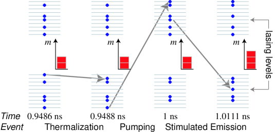
Figure 2: Four frames extracted from a Monte Carlo sequence for 10 equally-spaced energy levels in VB and CB. Time in arbitrary units increases from left to right. Insets give the number of light quanta $m$ stored in the cavity at some time. Arrows indicate electron displacements from one energy level to another.

The Fig. 2 illustrates three of these elementary processes by means of a sequence of four frames extracted from a computer simulation involving only 10 levels in each bands. At the start, the system has already reached a stationary regime. A sample of the electron distribution is shown on the left. The corresponding time and the number of light quanta stored in the cavity are respectively $\tau_{0}=0.9486$ ns and $m=2$. The first event at $\tau_{1}=0.9488$ ns is a VB thermalization. Its effect is to decrement the system energy of $\epsilon$ since an electron is demoted by one energy step. The second event at $\tau_{2}=1$ ns is an electrical pumping event that promotes the VB electron occupying the lowest energy level to the highest energy level of the CB. The third event illustrates stimulated emission between the prescribed lasing levels at $\tau_{3}=1.0111$ ns. As a result, the number of light quanta is incremented from $m=2$ to $m=3$.

Except for the pumping events all the processes are governed by a Poisson probability law. It follows that the whole system aside from pumping events also obeys a Poisson probability law. Knowledge of the laser microscopic state at time $\tau_{i}$ implies knowledge of the next-jump density function. An exact Monte Carlo simulation [6] of the laser evolution is then easily obtained by randomly picking up the next event time $\tau_{i+1}$ from a Poisson law and, next, picking the event type from a uniform law weighted by the count of potential events for each type. This method is more rigorous and more efficient than simulations based on infinitesimal time steps. The time required to obtain a photo-detection spectrum is on the order of a few hours on desk computers.

The times $t_{k}$ of occurrence of photo-detection events are registered once a steady-state regime has been reached, as is always the case for the kind of lasers considered. The detection rate $Q(t)$ is the sum over $k$ of $\delta(t-t_{k})$, where $\delta(.)$ denotes the Dirac distribution. Considering that the photo-detection events are part of a stationary process, the two-sided spectral density of the detection rate fluctuation $\Delta Q(t)\equiv Q(t)-\overline{Q}$ is [16]

$$S_{\Delta Q}(\Omega)=\frac{1}{T_{m}}\overline{\left|\sum_{k}\exp(-j\Omega t_{k})\right|^{2}}$$ (1)

where the overline stands for averaging and $\Omega\equiv 2\pi n/T_{m}$ with $n$ a nonzero integer. Note that $2S_{\Delta Q}(\Omega)df$, where $f\equiv\Omega/2\pi$, represents the power flowing out of a filter of width $df$ following the detector. For uniformly-distributed independent events, i.e. for a Poisson process, Eq. (1) gives the shot-noise formula $S_{\Delta Q}(\Omega)=\overline{Q}$.

4 Numerical Results

Simulations will be reported for three values of the thermalization parameter, namely $p=25\,000\;\text{ns}^{-1}$, $1\,000\;\text{ns}^{-1}$, $250\;\text{ns}^{-1}$, and $T=100$ K. Large values of $p$ enforce well-defined, constant temperatures to the electron gas. Conversely, small values of $p$ correspond to large carrier-lattice thermal resistances.

The total numbers of events during a run lasting 1 $\mu$s are, respectively, about $6.2\,10^{8}$, $3.9\,10^{7}$ and $1.1\,10^{7}$. The number of events of various kinds are listed in Table 1 for the three values of $p$ considered. The number of VB (resp., CB) “cooling” events is the number of downward electron transitions in the valence band (resp., conduction band) due to thermalization. Likewise, VB (resp., CB) “heating” refers to upward electron shifts.

The following observations can be made:

• The first two lines of the table show that, over a run, the number of detection events is essentially equal to the number of pumping events. Since the number of pumping events does not vary from run to run, it follows that the number of photo-detection events does not vary either, i.e., the light is “quiet”. Non-zero variances of the photo-count would appear only over much shorter durations.

• The next two lines show that the difference between the numbers of stimulated emission and absorption events is nearly equal to the number of photo-detection events. Because of the band symmetry, the numbers of stimulated events are almost independent of $p$.

• The difference between the number of cooling and heating events corresponds to the power delivered by the pump in excess of the power removed by the detector. This difference is almost independent of $p$.

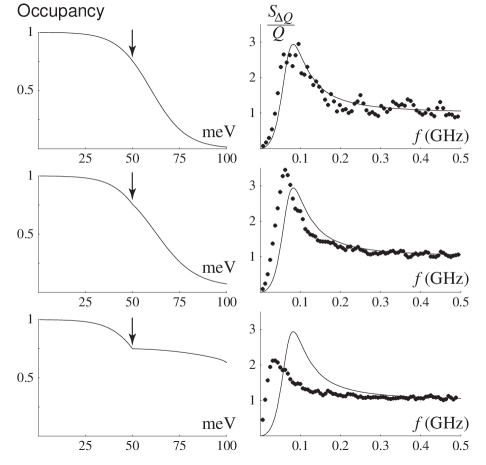
Figure 3: On the left, electron occupancy as a function of the energy referred to the bottom of the conduction band. Arrows point to the lasing level. On the right, normalized photo-detection spectra. Dots are Monte Carlo results and solid lines are from (24). The thermalization rates are $p=25\,000\;\text{ns}^{-1}$ (top), $1\,000\;\text{ns}^{-1}$ (middle), and $250\;\text{ns}^{-1}$ (bottom).

The CB level-occupancies are represented on the left-hand part of Fig. 3. The CB electron-occupancies and the VB hole occupancies are symmetrical with respect to the middle of the bandgap.

• For $p=25\,000\;\text{ns}^{-1}$, electron occupancies are very close to the Fermi-Dirac (FD) distribution, except near the edges of the band. A least-square fit shows that the carrier temperature is $T_{c}=105.6$ K for both bands. The quasi-Fermi levels (referred to the bottom of the bands) are respectively $\mu_{CB}=60.2$ and $\mu_{VB}=40.8$.

• For $p=1\,000\;\text{ns}^{-1}$, a fit gives $T_{c}=132$ K for both bands, $\mu_{CB}=63.5$ and $\mu_{VB}=37.5$. There is a dip due to ‘spectral hole burning’ (SHB) at the lasing level shown by an arrow. This dip is difficult to see on the figure, but it nevertheless influences importantly the noise properties of the laser.

• For $p=250\;\text{ns}^{-1}$, the dip at the lasing level is conspicuous.

The right part of Fig. 3 gives a comparison between spectra calculated from Monte Carlo data using Eq. (1) and the spectrum obtained from the elementary laser-diode noise theory (see the appendix) using the same set of parameters, $(\alpha,T,\epsilon,J)$. The top part of the figure corresponds to efficient thermalization. The spectral density is below the shot-noise level up to a frequency of 42 MHz. Notice the strong relaxation oscillation. There is good agreement between the Monte Carlo simulation and the linearized theory.

For moderate thermalizations the spectral density is below the shot-noise level up to a frequency of 25 MHz and no more agrees with the linearized theory. An increase of temperature from 100 K to 132 K does not suffice to reproduce the observed shift. The change in spectral density may be attributed to spectral-hole burning and carrier heating.

The bottom curve corresponds to poor thermalization. The relaxation oscillation is strongly damped. The frequency range where the spectral density is below the shot-noise level now extends only up to 8 MHz.

5 Conclusion

A Monte Carlo computer program keeping track of the occupancy of each level in the conduction and valence bands and of the number of light quanta in the optical cavity has been built. It has been applied to regularly-pumped mesoscopic laser diodes, having equally-spaced one-electron levels in each band. Numerical results have focused on laser noise, especially the spectral density of the photo-detection rate. When the electron-lattice thermal contact is good, theoretical results based on linearization and the Fermi-Dirac distribution are recovered. In particular, it is verified that sub-Poissonian light may be obtained. But when the thermal contact is poor, as is the case when lasers are driven to high powers, the simple theory is found to be inaccurate. Some of the changes observed may be accounted for by temperature increase and gain compression (due to spectral-hole burning). But unexpected effects are also found. In particular, an increase of the spectral density at low frequencies is noted. The program has been augmented to account for the intraband Auger effect that tends to ensure that the electron and hole temperatures are well defined, but possibly fluctuate differently in the course of time. It is also easy to take into account spontaneous carrier recombination and excess optical losses.

6 Appendix: Laser Diode Intensity Noise for the Case of Evenly-Spaced Electronic Levels.

A simple explicit expression for the spectral density of the photo-detection rate is presently derived. The theory of laser diode intensity noise for the case of non-fluctuating (or quiet) pumps was first given by Yamamoto and others [14] in 1986. A significantly simpler but strictly equivalent theory, based on rate equations, was subsequently given by Arnaud and Estéban [17]. The present appendix is based on the latter with some changes in the way the results are presented. Next, it will be shown that for electronic levels with even spacing $\epsilon$, the photo-detection spectrum depends on only two parameters, namely the dimensionless light quanta absorption constant $\alpha$ and a normalized pump rate $J^{\star}\equiv J\epsilon/k_{B}T$. As in the main text, the parameter $J$ denotes the pumping rate equal within our approximations to the average light-quanta output rate $Q$. In the present appendix ideal thermalization of the electron gas is assumed.

The main mechanisms involved in laser operation are stimulated emission and stimulated absorption. Einstein has shown that the probability that an electron in the lower working level be promoted to the empty upper working level is equal to the number $m$ of light quanta (or photons) in the optical cavity, defined as the ratio of the optical field energy and $\hbar\omega$, where $\hbar$ denotes the Planck constant divided by $2\pi$, and $\omega$ the angular frequency of oscillation. The probability that an electron in the upper level be demoted to the empty lower level is equal to $m+1$. These relations hold to within a constant common factor that we set equal to unity. This amounts to selecting a time unit. Because only far-above threshold operation is considered we have: $m\gg 1$ so that the “1” in the expression $m+1$ may be neglected. Spontaneous carrier recombination is first neglected, but expressions for spontaneous decay rates are given at the end of this appendix. From the present viewpoint, randomness in laser operation enters mainly because stimulated transitions obey probability rather than deterministic laws. The alternative interpretation of laser noise as resulting from the field spontaneously emitted into the oscillating mode, though plausible on some respects, does not seem able to lead in a natural manner to sub-Poissonian output light statistics, see [17].

In semiconductors it may happen that the two working levels are both occupied or that both are empty, in which cases no transition may occur. Stimulated absorption takes place when the lower level is occupied and the upper level is empty at an average rate denoted: $A\equiv L(n)m$. In the opposite situation, stimulated emission occurs at an average rate $E\equiv G(n)m$. Here $n$ denotes the total number of electrons in the conduction band. Because $m$ and $n$ are large integers and their relative fluctuations are small above threshold they may be viewed as continuous functions of time. It is also permissible to replace the average value of any smooth function $f(m,n)$ by $f(\overline{m},\overline{n})$. Overlines indicating that average values are considered will be omitted when no confusion is likely to arise, particularly in the expressions of spectral densities and after linearization of the equations. Stimulated absorption and emission rates read respectively

$$\mathcal{A}=L(n)m+a(t)\qquad\mathcal{E}=G(n)m+e(t)$$ (2)

The independent white noise sources $a(t)$ and $e(t)$ express the randomness of the transitions. Their spectral densities are equal to the average rates, that is, $S_{a}=A\equiv L(n)m$, $S_{e}=E\equiv G(n)m$.

If the optical cavity-semiconductor system were isolated (no pump, no optical absorption) the sum $n+m$ of the number of electrons $n$ in the conduction band and of the number $m$ of light quanta in the optical cavity would be a constant. It would then suffice to know the evolution equation for $m$ alone

$$\frac{dm}{dt}=\mathcal{R}\equiv\mathcal{E}-\mathcal{A}\equiv K(n)m+r(t)$$ (3)

where we have introduced the net gain

$$K(n)=G(n)-L(n)$$ (4)

The average number $\overline{n}$ of electrons follows from the steady-state condition: $K(\overline{n})=0$, while the average number of light quanta $\overline{m}$ would depend on the energy initially given to the isolated system. Because absorption and emission processes are independent, the spectral density of $r(t)\equiv e(t)-a(t)$ is the sum of the average rates

$$S_{r}=\left[G(n)+L(n)\right]m$$ (5)

But lasers are in fact open systems with a source of energy (the pump) and a sink of energy (the optical detector). To obtain the evolution equation for the number $m$ of light quanta one must subtract from the right-hand-side of (3) the loss rate $\mathcal{Q}$ due to the detector, no other optical loss being presently considered. Detection is a linear process of average rate $Q=\alpha m$ involving a noise term $q(t)$ whose spectral density equals the average rate. Accordingly

$$\mathcal{Q}\equiv\alpha m+q(t)\qquad S_{q}=Q=\alpha m$$ (6)

The parameter $\alpha$ represents the loss due to detector absorption. If the detector is located outside the cavity, $\alpha$ represents the loss due to transmission through partially transmitting mirrors.

The equation describing the evolution of the number $n$ of electrons in the conduction band, on the other hand, involves the constant pump rate $J$ (quiet pump). The two rate equations thus read

$$\frac{dm}{dt}=\mathcal{R}-\mathcal{Q}$$ (7)

$$\frac{dn}{dt}=J-\mathcal{R}$$ (8)

In the steady-state, the right-hand-sides of (7) and (8) vanish, and therefore

$$J=K(\overline{n})\overline{m}=\alpha\overline{m}\equiv Q$$ (9)

The above relation defines the steady-state values of $\overline{m}$ and $\overline{n}$, given $J=Q$, $\alpha$, and the $K(n)$ function.

For slow variations the left-hand-sides of the previous equations (7) and (8) may be neglected and thus $\mathcal{Q}(t)=J=\text{constant}$. In other words, the detection rate $\mathcal{Q}$ does not fluctuate when the pump is non-fluctuating or “quiet”. This simple result holds because carrier losses and light quanta losses, besides those due to detection, have been neglected. When the above equations are linearized and $\Delta m(t)\equiv m(t)-\overline{m}$, $\Delta n(t)\equiv n(t)-\overline{n}$ are Fourier transformed, one obtains

$$j\Omega\Delta m=\gamma\Delta n+r-q$$ (10)

$$j\Omega\Delta n=-\gamma\Delta n-K\Delta m-r$$ (11)

where $\Delta m$, $\Delta n$ are now functions of $\Omega$, and we have introduced the net differential gain

$$\gamma\equiv\frac{dK/dn}{K}$$ (12)

Let us recall that $r$ and $q$ are uncorrelated white-noise processes. Their spectral densities, $S_{r}$ and $S_{q}$, are given in (5) and (6), respectively.

The detection rate fluctuation $\Delta Q=\alpha\Delta m+q$ is obtained from (10) and (11) after elimination of $\Delta n$, as a weighted sum of the two independent white-noise terms $r$ and $q$, in the form: $\Delta Q=ar+bq$, where $a$ and $b$ denote two complex functions of $\Omega$. The spectral density of $\Delta Q$ is equal to $\lvert a\rvert^{2}S_{r}+\lvert b\rvert^{2}S_{q}$. Since the mathematical transformations has been given earlier [17] only the result is given below:

$$\frac{S_{\Delta Q}(\Omega)}{Q}=1+\frac{2n_{p}\Omega^{2}-\gamma^{2}m^{2}\alpha^{2}}{\gamma^{2}m^{2}\Omega^{2}+(\gamma m\alpha-\Omega^{2}/\alpha)^{2}}$$ (13)

where

$$n_{p}=\frac{G(n)}{K(n)}$$ (14)

denotes the population inversion (or “spontaneous emission”) factor, and $Q$ the average detection rate. This expression vanishes at $\Omega=0$ (quiet output). It is unity if $\Omega$ goes to infinity (i.e., the fluctuation is at the shot-noise level).

Let us now evaluate the parameters $\gamma$ and $n_{p}$ entering into the expression of the photo-detection rate spectrum. As in the main text model, each band is supposed to consist of $B$ one-electron levels separated in energy by a constant $\epsilon$. It is presently assumed that the conduction and valence electron temperatures remain at all times equal to the heat bath temperature $T$. This amounts to neglecting, besides temperature fluctuations, spectral-hole burning. The Fermi-Dirac distribution is applicable under the assumption that $\epsilon\ll k_{B}T\ll B\epsilon$. Under such conditions, the total number $n$ of electrons in the conduction band may be evaluated as if all levels above the quasi-Fermi level were empty and all levels below it were fully occupied (and likewise for the valence band). But stable laser operation is possible only if the net gain depends significantly on $n$. It is therefore essential to employ the exact Fermi-Dirac distribution when stimulated rates are being evaluated. Energies are counted upward from the bottom of the respective bands (see Fig. 1). Because of charge neutrality we have

$$n\epsilon=F_{c}=B\epsilon-F_{v}$$ (15)

This relation determines the quasi Fermi levels as functions of the number $n$ of electrons in the conduction band.

For definiteness, let us suppose that the two working levels are located at the middle of the conduction and valence bands, respectively, as shown on Fig. 1, that is: $k_{c}=k_{v}=B/2$. It follows from (15) that

$$\delta\equiv F_{c}-k_{c}\epsilon=k_{v}\epsilon-F_{v}$$ (16)

If we set

$$x\equiv\exp(-\frac{\delta}{k_{B}T})=\exp(\frac{B\epsilon/2-n\epsilon}{k_{B}T})$$ (17)

the upper and lower working level occupancies read respectively, according to the Fermi-Dirac formula

$$n_{c}=\frac{1}{1+x}\qquad n_{v}=\frac{x}{1+x}$$ (18)

Thus the stimulated gain and loss constants are

$$G(n)=n_{c}(1-n_{v})=\frac{1}{(1+x)^{2}}\qquad L(n)=n_{v}(1-n_{c})=\frac{x^{2}}{(1+x)^{2}}$$ (19)

and

$$K(n)\equiv G(n)-L(n)=\frac{1-x}{1+x}$$ (20)

The steady-state condition $K(\overline{n})=\alpha$ gives the steady-state value of $x$:

$$\overline{x}=\frac{1-\alpha}{1+\alpha}$$ (21)

The population inversion factor thus reads

$$n_{p}\equiv\frac{G}{K}=\frac{1}{1-\overline{x}^{2}}=\frac{(1+\alpha)^{2}}{4\alpha}$$ (22)

The differential gain parameter is obtained after derivation of $K(n)$ with respect to $n$ and rearranging as

$$\gamma=\frac{dK/dn}{K}=\frac{2}{x^{2}-1}\frac{dx}{dn}=\frac{\epsilon}{k_{B}T}\frac{2x}{1-x^{2}}=\frac{\epsilon}{k_{B}T}\frac{1-\alpha^{2}}{2\alpha}$$ (23)

When the above expressions of $n_{p}$ and $\gamma$ are introduced in (13) we finally obtain the photo-detection rate spectral density as a function of the frequency $f\equiv\Omega/2\pi$ with parameters $\alpha$ and $J^{\star}\equiv J\epsilon/k_{B}T$

$$\frac{S_{\Delta Q}(f)}{Q}=1+\frac{\frac{\alpha(1+\alpha)}{1-\alpha}\frac{F}{J^{\star}}-1}{\frac{1-\alpha^{2}}{2\alpha^{2}}J^{\star}F+\left(1-F\right)^{2}}$$ (24)

where $F\equiv\left(f/f_{r}\right)^{2}$, $\left(2\pi f_{r}\right)^{2}\equiv\frac{1-\alpha^{2}}{2}J^{\star}$ and $J^{\star}\equiv\frac{J\epsilon}{k_{B}T}$.

In the main text, very good agreement between the numerical simulation for a large thermalization parameter and the above analytical formulas was found. Typical parameter values are $\alpha=0.5$, $J^{\star}\approx 0.58$. Thus the relaxation frequency $f_{r}\approx 0.074$ GHz.

Within the present linearized theory, the spectrum would not be affected if there were many upper working levels in the conduction band instead of a single one, and likewise many lower working levels in the valence band. But when thermalization is poor the number of working levels in each band needs to be specified. Spectral-hole burning is indeed of lesser importance when the number of working levels is large.

If we suppose that spontaneous emission events satisfy the electron momentum conservation law, spontaneous carrier recombination occurs at an average rate $S(n)=\sigma n$ where the constant $\sigma$ depends on the optical density of mode, and thus on the dimensionality of the active region. This average rate should be supplemented with a noise term $s(t)$ whose spectral density is equal to the average rate. Auger spontaneous carrier recombinations would obey different laws not considered in this paper. Note that Monte Carlo simulations automatically account for all the noise sources associated with transition events.

Table 1: Number of events of various kinds during a $1\;\mu$s-run

$p$ (ns-1)	25 000	1 000	250
Pumping	5 000	5 000	5 000
Detection	5 004	5 000	5 000
Stimulated abs.	882	865	876
Stimulated emi.	5 883	5 865	5 876
VB “cooling”	155 286 151	9 819 009	2 848 060
VB “heating”	155 036 238	9 569 413	2 619 666
CB “cooling”	155 303 449	9 779 404	2 824 115
CB “heating”	155 058 595	9 534 806	2 599 576

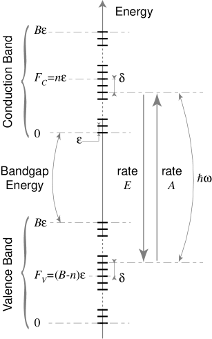
Figure 1: Schematic view of the energy level system considered.

References

- [1] S. Machida, Y. Yamamoto, and Y. Itaya, “Observation of amplitude squeezing in a constant-current driven semiconductor laser,” Phys. Rev. Lett., vol. 58, pp. 1000–1003, 1987.
- [2] J. Arnaud, “Photon-number variance in laser diodes with quiet pumps,” J. Opt. Soc. Am. B, vol. 14, pp. 2193–2196, 1997.
- [3] J. Arnaud, “Optically-pumped semiconductor squeezed-light generation,” Opt. Quant. Electron., vol. 27, pp. 225–238, 1995.
- [4] E. Jakeman and R. Loudon, “Fluctuations in quantum and classical populations,” J. Phys. A Math. Gen., vol. 24, pp. 5339–5347, 1991.
- [5] R. Loudon, The Quantum Theory of Light, Oxford University Press, Oxford, 1983.
- [6] D. T. Gillespie, Markov Processes: An Introduction for Physical Scientists, Academic Press, San Diego, 1992, see Chap. 6.
- [7] T. Ando, Y. Arakawa, K. Furuya, S. Komiyama, and H. Nakashima, Eds., Mesoscopic Physics and Electronics, Springer, Berlin, 1998.
- [8] C. Monat, X. Letartre, C. Seassal, J. Brault, M. Gendry, P. Rojo-Romeo, P. Pottier, and P. Viktorovitch, “Microsources optiques à base de cristaux photoniques et d’ilots quantiques InAs/InP,” in 20e Journées Nationales d’Optique Guidée, Toulouse, Nov. 2000, pp. 225–227.
- [9] R. Denton, B. Mühlschlegel, and D. J. Scalapino, “ ,” Phys. Rev. B, vol. 7, pp. 3589, 1973.
- [10] J. Arnaud, L. Chusseau, and F. Philippe, “Fluorescence from a few electrons,” Phys. Rev. B, vol. 62, pp. 13482–13489, 2000.
- [11] P. Meystre and M. Sargent III, Elements of Quantum Optics, Springer-Verlag, Berlin, 2nd edition, 1991.
- [12] M. Elk, “Numerical studies of the mesomaser,” Phys. Rev. A, vol. 54, pp. 4351–4358, 1996.
- [13] G. Giuliani, “Semiclassical particle-like description of optical amplifier noise,” Opt. Quant. Electron., vol. 31, pp. 367–376, 1999.
- [14] W. H. Richardson, S. Machida, and Y. Yamamoto, “Squeezed photon-number noise and sub-Poissonian electrical partition noise in a semiconductor laser,” Phys. Rev. Lett., vol. 66, pp. 2867–2870, 1991.
- [15] Y. Yamamoto and H. A. Haus, “Effect of electrical partition noise on squeezing in semiconductor lasers,” Phys. Rev. A, vol. 45, pp. 6596–6604, 1992.
- [16] A. Papoulis, Probability, Random Variables, and Stochastic Processes, MacGraw-Hill, New-York, 1965, see p. 367.
- [17] J. Arnaud and M. Estéban, “Circuit theory of laser diode modulation and noise,” IEE Proc. J, vol. 137, pp. 55–63, 1990.