Improved semiclassical density matrix: taming caustics

Abstract

We present a simple method to deal with caustics in the semiclassical approximation to the thermal density matrix of a particle moving on the line. For simplicity, only its diagonal elements are considered. The only ingredient we require is the knowledge of the extrema of the Euclidean action. The procedure makes use of complex trajectories, and is applied to the quartic double-well potential.

I Introduction

In the path integral formulation of quantum statistical mechanics, the thermal density matrix $\rho(x,x^{\prime})=\langle x|\exp(-\beta H)|x^{\prime}\rangle$ of a system with Hamiltonian

$$H=\frac{p^{2}}{2m}+V(x)$$ (1)

is given by [1, 2, 3]

$$\rho(x,x^{\prime})=\int_{z(0)=x^{\prime}}^{z(\beta\hbar)=x}[{\cal D}z(\tau)]\,\exp\left(-\frac{S[z]}{\hbar}\right),$$ (2)

with

$$S[z]=\int_{0}^{\beta\hbar}d\tau\left[\frac{1}{2}\,m\dot{z}^{2}+V(z)\right].$$ (3)

A semiclassical series for $\rho(x,x^{\prime})$ may be obtained from Eq. (2) through the method of steepest descent. The derivation depends solely on the knowledge of the paths that are minima of the Euclidean action $S$ (the Euclidean nature of the path integral allows us to discard saddle-points). They act as backgrounds upon which a semiclassical propagator can be obtained exactly and then used to construct the series perturbatively. Its first term is given by

$$\rho_{{\rm sc}}^{(1)}(x,x^{\prime})=\sum_{j=1}^{N}\exp\left(-\frac{S[x_{\rm c}^{j}]}{\hbar}\right)\Delta_{j}^{-1/2}.$$ (4)

The sum runs over all minima $x_{\rm c}^{j}(\tau)$ of the action $S[z]$ satisfying the boundary conditions $z(0)=x^{\prime}$ and $z(\beta\hbar)=x$, and $\Delta_{j}$ denotes the determinant of

$$\hat{F}[x_{\rm c}^{j}]\equiv-m\,\frac{d^{2}}{d\tau^{2}}+V^{\prime\prime}[x_{\rm c}^{j}],$$ (5)

the operator of quadratic fluctuations around $x_{\rm c}^{j}(\tau)$. (A derivation of this result will be sketched in Sec. II.)

In previous works [4, 5], we presented the explicit construction of the series for the diagonal elements of the density matrix, $\rho(x,x)$. For the sake of simplicity, we restricted our discussion to potentials of the single-well type. The more intricate case of multiple-wells — of which the quartic double well, with its many applications of practical importance [6], is a paradigm — was left aside, as it requires special treatment. Differently from single-wells, for multiple-wells the number $N$ of minima of $S$ depends on $x$ and $\beta$ [7]. On the frontier separating regions in the $(x,\beta)$-plane with different values of $N$ — a caustic — $\rho_{{\rm sc}}(x,x)$ diverges due to the vanishing of the fluctuation determinant around the minimum that appears or disappears there. In the present context, this divergence is an artifact of the semiclassical approximation. Thus, a simple manner of eliminating it is certainly called for; this is the purpose of this paper.

As the caustic problem appears in other contexts in physics, it is instructive to briefly review how it comes about, and how it has been dealt with, for the sake of comparison. In optics, caustics occur whenever light rays coalesce. Thus, they separate regions of different number of extrema (the light rays) of the optical distance (the analogue of the action). In order to go beyond geometrical optics, one has to take into account fluctuations around these light rays. Just as in the present case, singularities emerge when we compute quadratic fluctuations on caustics. Ways to avoid this have been known for some time [8, 9, 10, 11, 12]. Indeed, due to the traditional analogy between wave optics and quantum mechanics, the techniques involved are similar to the ones used in deriving connection formulae for WKB approximations [13], and consist essentially in replacing one or more of the Fresnel integrals that arise in the stationary phase approximation with a so-called diffraction integral, whose form is specified by the classification of the caustic according to Catastrophe Theory [14, 15]; in the simplest case it is an Airy-type integral. A general procedure has also been developed to deal with caustics in the path integral formulation of quantum mechanics [16]. Although this general procedure could, in principle, be adapted to the case at hand, the nature of our problem allows for simplifications which warrant special treatment.

In nonequilibrium quantum statistical mechanics, caustics are also known to occur in semiclassical descriptions of the decay of metastable states. The problem here is that of a particle in a potential which has a local minimum separated by a barrier from a region where it is unbounded below, in contact with a thermal reservoir. The phenomenon of caustics has been associated with a transition from the classical to the quantum regime of the decay rate [17, 18, 19]. General prescriptions for dealing with this phenomenon near the top of the barrier have been given in great detail [19, 20, 21].

The case we shall analyze in this article differs from the one in the previous paragraph in the following aspects: (i) we discuss a problem in equilibrium quantum statistical mechanics; (ii) our analysis is global, in the sense that we compute the density matrix diagonal for every point on the real axis. It also differs from analyses carried out in optics and quantum mechanics because of the Euclidean nature of the path integral: only minima are to be considered; saddle-points are discarded. (This is strictly true only in the “usual” semiclassical approximation. Our “improved” approximation makes use of some of the saddle-points.) In fact, in the specific example we analyze (the quartic double-well potential) only one new (local) minimum is introduced in function space after the various catastrophes that occur as we change the temperature; as it appears after the first catastrophe, this is the only one we have to consider. (Again, this is valid only for the “usual” semiclassical approximation; the improved one also requires an analysis of the second catastrophe.) This results in a prescription for dealing with caustics that is simple and direct.

Previous works have studied the quartic double-well potential at finite temperature using semiclassical methods [22, 23]. Our work complements and extends those studies, by giving an explicit recipe for dealing with caustics. Variational methods have also proven extremely useful in this problem, and were quite successful in addressing applications in condensed matter physics [24]. Combinations of perturbation theory with variational techniques have also been recently used [25]. Our contribution to the semiclassical treatment opens the way for practical calculations, to be compared with perturbative, variational and numerical results.

This article is organized as follows: before introducing the improved semiclassical approximation, which will remedy the problem of spurious divergences, Sec. II briefly reviews the derivation of the usual semiclassical approximation to the density matrix. The new method is, then, presented in two alternative ways: one has a better physical motivation, and clearly illustrates the essential ideas, but lacks effectiveness as a calculational tool; the other provides a general recipe to perform the calculations in a systematic way, resorting to the use of complex trajectories. Sec. III describes in detail the results obtained for the case of the quartic double-well potential by using the improved semiclassical approximation, which are compared to the usual approach. Sec. IV presents our conclusions and points out directions for future work.

II Improving the semiclassical approximation

A The “usual” semiclassical approximation

In order to show how one can improve the semiclassical approximation so as to eliminate the unphysical divergences at the caustics, it is convenient to remember how the usual semiclassical approximation to a path integral like the one in Eq. (2) is derived. Briefly, one has to:

(A) Solve the Euler-Lagrange equation, $m\ddot{z}=V^{\prime}(z)$, subject to the boundary conditions $z(\beta\hbar)=z(0)=x$, and determine, among the solutions, those which minimize (globally or locally) the action. For simplicity, we shall assume for the moment that there is only one such solution, which we denote by $x_{\rm c}$;

(B) Expand the action around $x_{\rm c}$: $S[x_{\rm c}+\eta]=S[x_{\rm c}]+S_{2}+\delta S$, where

$$S_{2}=\frac{1}{2}\int_{0}^{\beta\hbar}d\tau\,\eta(\tau)\,\hat{F}[x_{\rm c}]\,\eta(\tau),$$ (6)

$$\delta S=\sum_{k=3}^{\infty}\frac{1}{k!}\int_{0}^{\beta\hbar}d\tau\,V^{(k)}[x_{\rm c}(\tau)]\,\eta^{k}(\tau);$$ (7)

$\hat{F}$ is the operator defined in Eq. (5), and we are assuming that $V(z)$ is an analytic function of $z$, so that all derivatives $V^{(k)}(z)$ exist;

(C) Expand the fluctuations $\eta(\tau)$ in terms of the orthonormal modes of the fluctuation operator $\hat{F}[x_{\rm c}]$:

$$\eta(\tau)=\sum_{j=0}^{\infty}a_{j}\varphi_{j}(\tau),$$ (8)

where $\hat{F}\varphi_{j}(\tau)=\lambda_{j}\varphi_{j}(\tau)$, with $\varphi_{j}(0)=\varphi_{j}(\beta\hbar)=0$; then

$$S_{2}=\frac{1}{2}\sum_{j=0}^{\infty}\lambda_{j}a_{j}^{2},$$ (9)

$$\delta S=\sum_{n=3}^{\infty}\sum_{i_{1}=0}^{\infty}\cdots\sum_{i_{n}=0}^{\infty}\frac{1}{n!}\,C^{(n)}_{i_{1}i_{2}\ldots i_{n}}\,a_{i_{1}}a_{i_{2}}\ldots a_{i_{n}},$$ (10)

where

$$C^{(n)}_{i_{1}\ldots i_{n}}=\int_{0}^{\beta\hbar}d\tau\,V^{(n)}[x_{\rm c}(\tau)]\,\varphi_{i_{1}}(\tau)\ldots\varphi_{i_{n}}(\tau).$$ (11)

The “usual” semiclassical approximation is obtained by neglecting $\delta S$ in the path integral on the r.h.s. of Eq. (2), which, upon the change of variables $\eta(\tau)\to\{a_{j}\}$, becomes a product of Gaussian integrals:

$$\rho(x,x)\approx\exp\left(-\frac{S[x_{\rm c}]}{\hbar}\right)\prod_{j=0}^{\infty}{\cal I}_{j}\>,$$ (12)

$${\cal I}_{j}=\int_{-\infty}^{\infty}\frac{da_{j}}{\sqrt{2\pi\hbar}}\,\exp\left(-\frac{\lambda_{j}a_{j}^{2}}{2\hbar}\right)=\lambda_{j}^{-1/2}.$$ (13)

Hence

$$\rho(x,x)\approx\exp\left(-\frac{S[x_{\rm c}]}{\hbar}\right)\Delta^{-1/2},$$ (14)

where $\Delta=\prod_{j=0}^{\infty}\lambda_{j}={\rm det}\,\hat{F}$. (Explicit expressions for $\Delta$ [see Eq. (42) below] were derived in Ref. [4], where it was also discussed how to systematically include corrections due to $\delta S$.) If there are $N$ minima, one has to add together their contributions, thus obtaining Eq. (4).

B Taming the caustics

When we cross a caustic, a classical trajectory $x_{\rm c}(\tau)$ is created or annihilated. Precisely at this point, the lowest eigenvalue of $\hat{F}[x_{\rm c}]$ vanishes, thus making the integral ${\cal I}_{0}$ blow up. This problem can be remedied by retaining fluctuations beyond quadratic in the subspace spanned by $\varphi_{0}$ (the eigenmode of $\hat{F}$ associated with $\lambda_{0}$), i.e., we replace ${\cal I}_{0}$ with

$$\widetilde{\cal I}_{0}=\int_{-\infty}^{\infty}\frac{da_{0}}{\sqrt{2\pi\hbar}}\,\exp\left(-\frac{{\cal V}(a_{0})}{\hbar}\right)\equiv\lambda_{0}^{-1/2}\,{\cal F},$$ (15)

where

$${\cal V}(a_{0})=\frac{1}{2}\,\lambda_{0}a_{0}^{2}+\sum_{n=3}^{M}\frac{1}{n!}\,C^{(n)}_{00\ldots 0}\,a_{0}^{n}.$$ (16)

We take for $M$ the smallest even integer such that $C^{(M)}_{00\ldots 0}$ is positive for all values of $x_{0}$ and $\beta$; this suffices to make the integral in (15) finite even when $\lambda_{0}$ vanishes.

As a result, we obtain an improved approximation to the density matrix element (2):

$$\rho(x,x)\approx\exp\left(-\frac{S[x_{\rm gm}]}{\hbar}\right)\Delta^{-1/2}\,{\cal F}.$$ (17)

Here, $x_{\rm gm}$ is the global minimum of $S[x]$.

It is important to note that there is a one-to-one correspondence between the minima of $S[x]$ and the minima of ${\cal V}(a_{0})$. Therefore, it is not necessary to explicitly add their contributions as in Eq. (4), for they are already included in (17). Indeed, let $a_{01}(=0),a_{02},\ldots,a_{0N}$ be the minima of ${\cal V}$. If they are sufficiently far apart, one may compute ${\cal F}$ using the steepest descent method, obtaining

$${\cal F}\sim\sum_{j=1}^{N}\sqrt{\frac{\lambda_{0}}{{\cal V}^{\prime\prime}(a_{0j})}}\,\exp\left(-\frac{{\cal V}(a_{0j})}{\hbar}\right)$$ (18)

Substituting this into Eq. (17) then yields

$$\rho(x,x)\approx\sum_{j=1}^{N}\exp\left(-\frac{S_{j}}{\hbar}\right)\widetilde{\Delta}_{j}^{-1/2},$$ (19)

where $S_{j}\equiv S[x_{\rm gm}]+{\cal V}(a_{0j})$ and $\widetilde{\Delta}_{j}\equiv({\cal V}^{\prime\prime}(a_{0j})/\lambda_{0})\,\Delta$. Although expression (19) is not identical to the “usual” semiclassical approximation [Eq. (4)], the dominant term in both sums is the same, namely $\exp(-S[x_{\rm gm}]/\hbar)\,\Delta^{-1/2}$ (recall that $a_{01}=0$, hence ${\cal V}(a_{01})=0$ and ${\cal V}^{\prime\prime}(a_{01})=\lambda_{0}$); the other terms are exponentially supressed in the classical limit $\hbar\to 0$.

Another point that is important to mention is that one can, in principle, systematically improve the “improved” semiclassical approximation, Eq. (17). To do this, one first decomposes the action into three pieces: $S[x_{\rm gm}+\eta]=S[x_{\rm gm}]+S_{\rm I}+S_{\rm II}$, where

$$S_{\rm I}={\cal V}(a_{0})+\frac{1}{2}\sum_{j=1}^{\infty}\lambda_{j}a_{j}^{2}$$ (20)

and

$$S_{\rm II}=\delta S-\left[{\cal V}(a_{0})-\frac{1}{2}\,\lambda_{0}a_{0}^{2}\right],$$ (21)

with $\delta S$ defined by Eq. (10). Applying this decomposition to Eq. (2) (with $x^{\prime}=x$) then yields

$$\rho(x,x)=\exp\left(-\frac{S[x_{\rm gm}]}{\hbar}\right)\int\prod_{j=0}^{\infty}\frac{da_{j}}{\sqrt{2\pi\hbar}}\,\exp\left(-\frac{S_{\rm I}}{\hbar}\right)\sum_{n=0}^{\infty}\frac{1}{n!}\left(-\frac{S_{\rm II}}{\hbar}\right)^{n}.$$ (22)

This defines an “improved semiclassical series,” the first term of which corresponds to Eq. (17). Higher order terms can be readily computed, as they can be recast as sums of products of simple integrals. Compared with the “usual” semiclassical series [4], the series (22) has the disadvantage that integrals involving powers of $a_{0}$ must be computed numerically. On the other hand, those integrals are finite even at the caustics, so that the coefficients of the series (22) are well defined for any $\beta$ and $x_{0}$.

Although the procedure outlined in this subsection teaches us how to cross the caustics, it is not very convenient: in order to obtain the coefficients of ${\cal V}(a_{0})$ one has to find $\lambda_{0}$ and $\varphi_{0}(\tau)$. This, in general, is not an easy task, and makes the whole procedure very cumbersome. Instead, we shall present an alternative way of obtaining those coefficients, which is based on the one-to-one correspondence between the minima of $S$ and ${\cal V}$.

C An alternative procedure

Let us assume that $M=4$ in Eq. (16); this is the case for the quartic double-well potential, to be discussed in the next section. Then the “effective action” ${\cal A}(a_{0})\equiv S[x_{\rm gm}]+{\cal V}(a_{0})$ for the “critical” mode $\varphi_{0}$ is a fourth degree polynomial in $a_{0}$.

Let us also assume for the moment that ${\cal A}(a_{0})$ has three extrema: a global minimum at $a_{0}=0$, a local maximum at $u>0$, and a local minimum at $v>u$. This allows us to write ${\cal A}(a_{0})$ as

$${\cal A}(a_{0})=S[x_{\rm gm}]+\alpha\left[\frac{1}{2}\,uv\,a_{0}^{2}-\frac{1}{3}\,(u+v)\,a_{0}^{3}+\frac{1}{4}\,a_{0}^{4}\right]$$ (23)

(one can easily check that ${\cal A}^{\prime}(0)={\cal A}^{\prime}(u)={\cal A}^{\prime}(v)=0$).

We now have to relate $\alpha$, $u$, and $v$ to calculable quantities. We do this by imposing that ${\cal A}(v)=S[x_{\rm lm}]$ and ${\cal A}(u)=S[x_{\rm sp}]$, where $x_{\rm lm}(\tau)$ and $x_{\rm sp}(\tau)$ are the local minimum and the lowest saddle-point of $S[x]$, respectively. This yields

$$\frac{S[x_{\rm lm}]-S[x_{\rm gm}]}{S[x_{\rm sp}]-S[x_{\rm gm}]}=\frac{{\cal A}(v)-{\cal A}(0)}{{\cal A}(u)-{\cal A}(0)}=\frac{\xi^{3}(2-\xi)}{2\xi-1},$$ (24)

where $\xi\equiv v/u$. It follows from the definition of $x_{\rm gm}$, $x_{\rm lm}$ and $x_{\rm sp}$ that the l.h.s. of Eq. (24) is in the range $[0,1]$. A plot of its r.h.s. shows that Eq. (24) possesses a unique real solution, lying in the interval $1\leq\xi\leq 2$.

Having determined $\xi$, we can now fix another combination of parameters, namely $\mu\equiv\alpha u^{4}$:

$$S[x_{\rm sp}]-S[x_{\rm gm}]={\cal A}(u)-{\cal A}(0)=\frac{\mu}{12}\,(2\xi-1).$$ (25)

We can then rewrite (23) as ${\cal A}(a_{0})=S[x_{\rm gm}]+{\cal V}_{3}(a_{0}/u)$, where

$${\cal V}_{3}(z)\equiv\mu\left[\frac{1}{2}\,\xi z^{2}-\frac{1}{3}\,(1+\xi)\,z^{3}+\frac{1}{4}\,z^{4}\right].$$ (26)

There still remains one parameter to be determined, namely $u$. Fortunately, we do not need it in order to compute ${\cal F}$. Indeed, identifying ${\cal V}_{3}(a_{0}/u)$ with ${\cal V}(a_{0})$ yields $\lambda_{0}=\mu\xi/u^{2}$, so that

$${\cal F}=\sqrt{\frac{\mu\xi}{2\pi\hbar u^{2}}}\int_{-\infty}^{\infty}da_{0}\,\exp\left(-\frac{{\cal V}_{3}(a_{0}/u)}{\hbar}\right).$$ (27)

Changing the variable of integration to $z=a_{0}/u$ eliminates the unknown parameter $u$ from the problem, leaving us with an expression for ${\cal F}$ which depends only on the calculable parameters $\xi$ and $\mu$:

$${\cal F}=\sqrt{\frac{\mu\xi}{2\pi\hbar}}\int_{-\infty}^{\infty}dz\,\exp\left(-\frac{{\cal V}_{3}(z)}{\hbar}\right).$$ (28)

The case in which $S$ has only one extremum can be dealt with similarly. Now ${\cal A}^{\prime}(a_{0})$ has one real root ($a_{0}=0$), corresponding to the minimum $x_{\rm gm}(\tau)$ of $S[x]$, and a pair of complex conjugate roots, $w$ and $w^{*}$, corresponding to the pair of complex conjugate trajectories $x_{\rm ct}(\tau)$ and $x_{\rm ct}^{*}(\tau)$. Correspondingly, we have ${\cal A}(a_{0})=S[x_{\rm gm}]+{\cal V}_{1}(a_{0}/|w|)$, where

$${\cal V}_{1}(z)\equiv\chi\left[\frac{1}{2}\,z^{2}-\frac{2}{3}\,(\cos\phi)\,z^{3}+\frac{1}{4}\,z^{4}\right],$$ (29)

with $\chi\equiv\alpha|w|^{4}$ and $\phi\equiv{\rm arg}(w)$. Identifying ${\cal A}(w)$ with $S[x_{\rm ct}]$ yields

$$S[x_{\rm ct}]-S[x_{\rm gm}]=\frac{\chi}{12}\left(2e^{2i\phi}-e^{4i\phi}\right),$$ (30)

from which we can obtain $\chi$ and $\phi$. Finally, identifying ${\cal V}_{1}(a_{0}/|w|)$ with ${\cal V}(a_{0})$ yields $\lambda_{0}=\chi/|w|^{2}$, which leads to

$${\cal F}=\sqrt{\frac{\chi}{2\pi\hbar|w|^{2}}}\,\int_{-\infty}^{\infty}da_{0}\,\exp\left(-\frac{{\cal V}_{1}(a_{0}/|w|)}{\hbar}\right)=\sqrt{\frac{\chi}{2\pi\hbar}}\,\int_{-\infty}^{\infty}dz\,\exp\left(-\frac{{\cal V}_{1}(z)}{\hbar}\right).$$ (31)

In the jargon of Ref. [7], the solution we have called $x_{\rm lm}(\tau)$ is a one-saddle: the operator of quadratic fluctuations around it, $\hat{F}[x_{\rm lm}]$, has only one negative eigenvalue. At the second catastrophe, the one-saddle becomes a two-saddle (i.e., it becomes unstable in another direction in the functional space), and two one-saddles appear. Having lower action than the two-saddle, the one-saddles have a larger weight in the partition function. Hence, when the second caustic is crossed the role of “lowest saddle-point” in Eqs. (24) and (25) is transferred to one of the newly born one-saddles, namely the one with the lowest action. The transition is smooth as all three trajectories coalesce and thus are identical to each other at the caustic. We also notice that, in spite of the infinite number of catastrophes, such a change of roles occurs only once, namely at the second catastrophe, since the minima of $S$ and the one-saddles do not take part in the subsequent catastrophes. Indeed, as shown in Ref. [7] (see also Sec. III B 5), only $(n-1)$-saddles and $n$-saddles take part in the $n$-th catastrophe.

III Application: the quartic double-well potential

A Preliminaries

Let us consider the quartic double-well potential, given by

$$V(x)=\frac{\lambda}{4}\,(x^{2}-a^{2})^{2}\qquad(\lambda>0).$$ (32)

In order to simplify notation, it is convenient to replace $x$ and $\tau$ by $q\equiv x/a$ and $\theta\equiv\omega\tau$, respectively, with $\omega\equiv(\lambda a^{2}/m)^{1/2}$. In the new variables, the equation of motion reads $\ddot{q}=U^{\prime}(q)$, where $U(q)\equiv\frac{1}{4}\,(q^{2}-1)^{2}$. Its first integral is

$$\frac{1}{2}\,\dot{q}^{2}=U(q)-U(q_{\rm t}),$$ (33)

where $q_{\rm t}$ denotes the turning point (i.e., the point where $\dot{q}=0$). This can be further integrated to give us the relation between $q_{\rm t}$ and the initial position $q_{0}$ for a given “time of flight” $\Theta\equiv\beta\hbar\omega$. (As shown in Ref. [4], that relation is all we need in order to compute the “usual” semiclassical approximation to $\rho(x,x)$, Eq. (4). The same is true for the computation of the improved approximation, Eq. (17), using the procedure outlined in Sec. II C.) Assuming for the moment that $0\leq q_{0}\leq q_{\rm t}\leq 1$, we can write

$$\frac{\Theta}{2}=\int_{q_{0}}^{q_{\rm t}}\frac{dq}{\sqrt{2[U(q)-U(q_{\rm t})]}}.$$ (34)

Inserting the explicit form of $U(q)$ and changing the integration variable to $z=q/q_{\rm t}$, Eq. (34) becomes

$$u=\int_{q_{0}/q_{\rm t}}^{1}\frac{dz}{\sqrt{(1-z^{2})(1-k^{2}z^{2})}}\,,$$ (35)

where

$$u\equiv\frac{\Theta}{2}\sqrt{1-\frac{1}{2}\,q_{\rm t}^{2}}\,,\qquad k^{2}\equiv\frac{q_{\rm t}^{2}}{2-q_{\rm t}^{2}}\,.$$ (36)

Performing the integration (formula 130.13 of Ref. [27]) and solving for $q_{0}$ finally yields

$$q_{0}=q_{\rm t}\,{\rm cd}(u,k),$$ (37)

where ${\rm cd}$ is one of the Jacobian elliptic functions.

The action can be written as $S[x]=(\hbar/g)\,I[q]$, where $g\equiv\hbar\lambda/m^{2}\omega^{3}$ and

$$I[q]=\int_{0}^{\Theta}d\theta\left[\frac{1}{2}\,\dot{q}^{2}+U(q)\right].$$ (38)

Using Eq. (33), we may rewrite $I[q_{\rm c}]$ as

$$I[q_{\rm c}]=\Theta\,U(q_{\rm t})+2\int_{q_{0}}^{q_{\rm t}}dq\,\sqrt{2\,[U(q)-U(q_{\rm t})]}.$$ (39)

The integration can be done with the help of formula 219.11 of Ref. [27]. After a few algebraic manipulations one arrives at

$$I[q_{\rm c}] = \Theta\,U(q_{\rm t})-\frac{1}{3}\,\sqrt{2\,q_{0}^{2}\,(q_{\rm t}^{2}-q_{0}^{2})(2-q_{\rm t}^{2}-q_{0}^{2})}$$ (41)

$$-\frac{2}{3}\,\sqrt{2(2-q_{\rm t}^{2})}\left\{(1-q_{\rm t}^{2})\,[{\rm K}(k)-{\rm F}(\varphi,k)]-{\rm E}(k)+{\rm E}(\varphi,k)\right\},$$

where K, F and E are elliptic integrals [26, 27] and $\varphi=\arcsin(q_{0}/q_{\rm t})$.

Equations (37) and (41) have been derived under the assumption that $q_{0}$ and $q_{\rm t}$ are real and satisfy $0\leq q_{0}\leq q_{\rm t}\leq 1$. However, since the elliptic functions and integrals are meromorphic functions of their arguments, we can now abandon that assumption and treat $q_{0}$ and $q_{\rm t}$ as complex variables. (Note, however, that $I[q_{\rm c}]$ is a multivalued function of $q_{\rm t}$ and so one must be a bit careful when computing it. For instance, the first square root in Eq. (41) acquires a minus sign if $-1<q_{\rm t}<-q_{0}<0$.)

Finally, the determinant of the fluctuation operator is given by [4]

$$\Delta=4\pi g\,{\rm sgn}(q_{0}-q_{\rm t})\,\frac{\sqrt{2\,[U(q_{0})-U(q_{\rm t})]}}{U^{\prime}(q_{\rm t})}\left(\frac{\partial q_{0}}{\partial q_{\rm t}}\right)_{\Theta}.$$ (42)

We now have all the ingredients to compute the semiclassical approximation to $\rho(x,x)$ — both the “usual” and the “improved” one. Indeed, both the action and the determinant of fluctuations can be expressed solely in terms of $q_{\rm t}$. Therefore, as anticipated, this is the only information we need from the classical trajectories.

B Singularities and their removal

As we have already said, the “usual” semiclassical approximation to $\rho(q_{0},q_{0})$ diverges at a caustic because of the vanishing of the determinant of fluctuations $\Delta$ around the minimum of $S$ which appears or disappears there. According to Eq. (42), there are two ways $\Delta$ may vanish: (i) when $(\partial q_{0}/\partial q_{\rm t})_{\Theta}=0$; (ii) when $U(q_{0})=U(q_{\rm t})$. A qualitative analysis of the equation of motion shows that, at the boundary between the $N=1$ and the $N=2$ regions in the $(q_{0},\Theta)$-plane, $\Delta$ vanishes according to the first alternative [7]. Solving the equation $(\partial q_{0}/\partial q_{\rm t})_{\Theta}=0$ for $q_{\rm t}$ and inserting the result $\tilde{q}_{\rm t}(\Theta)$ into Eq. (37), one obtains the lower curve depicted in Fig. 1 — the caustic.

In what follows we shall examine the behavior of the “usual” semiclassical approximation across the caustic, and compare it with the improved approximation. (All numerical calculations were performed using maple.)

1 $q_{0}=0$, $\Theta\approx\pi$

When $q_{0}=0$ and $\Theta<\pi$, the only real solution to Eq. (37) is $q_{\rm t}=0$. It then follows from Eq. (39) that $I[q_{\rm c}]=\Theta/4$. In order to compute $\Delta$ we need $q_{0}(q_{\rm t},\Theta)$ for small $q_{\rm t}$. Using Eqs. (36) and (37) we find $q_{0}\approx q_{\rm t}\,{\rm cd}(\Theta/2,0)=q_{\rm t}\,\cos(\Theta/2)$; Eq. (42) then yields $\Delta=2\pi g\,\sin\Theta$ in the limit $q_{\rm t}\to 0$. Therefore, the “usual” semiclassical approximation to $\rho(0,0)$ gives

$$\rho_{{\rm sc}}(0,0)\approx(2\pi g\,\sin\Theta)^{-1/2}\,\exp\left(-\frac{\Theta}{4g}\right)\qquad(\Theta<\pi).$$ (43)

It diverges like $(\pi-\Theta)^{-1/2}$ as $\Theta\to\pi^{-}$.

While for $\Theta<\pi$ there is only one real solution to the equation $q_{0}(q_{\rm t},\Theta)=0$, for $\Theta>\pi$ there are three: $q_{\rm t}=0$, corresponding to the trajectory $q_{\rm c}(\theta)\equiv 0$ (which is now a 1-saddle), plus a pair of solutions located symmetrically with respect to the origin, corresponding to a pair of degenerate minima of the action (see Fig. 2). The latter can be traced back to a pair of purely imaginary trajectories for $\Theta<\pi$. Indeed, making $q_{\rm t}=i\xi$ in Eqs. (36)–(37) and using the identity ${\rm cd}(u,ik)={\rm cn}(u\,\sqrt{1+k^{2}},k/\sqrt{1+k^{2}})$ [27], we obtain

$$q_{0}=i\xi\,{\rm cn}\left(\frac{\Theta}{2}\,\sqrt{1+\xi^{2}},\frac{\xi}{\sqrt{2(1+\xi^{2})}}\right).$$ (44)

The r.h.s. of the above equation has an infinite number of zeros besides the one at $\xi=0$ (see Fig. 3). As $\Theta$ approaches $\pi$ from below, the zeros approach the origin and two of them eventually coalesce there when $\Theta=\pi$, reappearing as a pair of real solutions to the equation $q_{0}(q_{\rm t},\Theta)=0$ for $\Theta>\pi$.

In Fig. 4 we show both the usual [Eq. (4)] and the improved [Eq. (17)] semiclassical approximation to $\rho(0,0)$ for $\Theta\approx\pi$.

2 $\Theta=\pi$, $q_{0}\approx 0$

When $\Theta=\pi$, the approximation $q_{0}\approx q_{\rm t}\,\cos(\Theta/2)$ is not enough for our purposes. Going to the next nontrivial order in the Taylor expansion of $q_{0}(q_{\rm t},\pi)$ one obtains $q_{0}\sim q_{\rm t}^{3}$ as $q_{\rm t}\to 0$. It then follows from Eqs. (4), (41) and (42) that the usual semiclassical approximation to $\rho(q_{0},q_{0})$ behaves, for $\Theta=\pi$, as

$$\rho_{{\rm sc}}(q_{0},q_{0})\stackrel{{\scriptstyle q_{0}\to 0}}{{\sim}}g^{-1/2}\,|q_{0}|^{-1/3}\,\exp\left(-\frac{\pi}{4g}\right).$$ (45)

Two aspects of this result are worth of mention: (i) the singularity at $q_{0}=0$ is integrable, hence the semiclassical partition function is well defined; (ii) because of the exponential factor, if $g\ll 1$ one has to be very close to the origin to “notice” the singularity: for $\rho_{{\rm sc}}(q_{0},q_{0})$ to be of order unity or greater, $q_{0}$ must satisfy $|q_{0}|\lesssim g^{-3/2}\,\exp(-3\pi/4g)$.

Fig. 5 shows both the usual and the improved semiclassical approximation to $\rho(q_{0},q_{0})$ for $\Theta=\pi$. In order to make visible the singular behavior of the former, we have taken $g=0.3$. One can notice that far from the caustic (i.e., for $q_{0}\gtrsim 0.2$) the two curves are similar, but differ by approximately $10\%$. This is due to the relatively large value of $g$. The difference becomes smaller as $g$ is made smaller, and vanishes in the classical limit $g\to 0$.

3 $\Theta>\pi$

Expanding $q_{0}(q_{\rm t},\Theta)$ around $\tilde{q}_{\rm t}(\Theta)$, we obtain $q_{0}-\tilde{q}_{0}\sim(q_{\rm t}-\tilde{q}_{\rm t})^{2}$, so that $\partial q_{0}/{\partial q_{\rm t}}\sim(q_{\rm t}-\tilde{q}_{\rm t})$ near the caustic. The other terms in Eq. (42) remain finite on it, so that we finally obtain

$$\Delta^{-1/2}\sim|q_{\rm t}-\tilde{q}_{\rm t}|^{-1/2}\sim|q_{0}-\tilde{q}_{0}|^{-1/4}.$$ (46)

Fig. 6 depicts both the usual and the improved semiclassical approximation to $\rho(q_{0},q_{0})$ for $\Theta=5.0$. Again we had to use a relatively large value of $g$ in order to magnify the “critical” region where the usual semiclassical result diverges. Note that the divergence occurs only at the two minima side of the caustic (see Fig. 7), as it is associated with the coalescence of the local minimum with a saddle-point of the action; the contribution of the global minimum remains finite at the caustic.

4 $\Theta\geq 2\pi$

As discussed in Ref. [7], another catastrophe is present if $\Theta\geq 2\pi$. This time, $\Delta$ vanishes when the classical trajectory is such that $U(q_{0})=U(q_{\rm t})$, or, since the potential is symmetric about the origin, $q_{\rm t}=-q_{0}$. This catastrophe is associated with the appearance of periodic classical trajectories, and the condition $q_{\rm t}=-q_{0}$ determines the amplitude $A(\Theta)$ of these trajectories [$A(\Theta)$ is the positive solution to equation $q_{0}(q_{\rm t},\Theta)=-q_{\rm t}$, where $q_{0}(q_{\rm t},\Theta)$ is defined by Eqs. (36) and (37)]. It is not difficult to see why a catastrophe occurs when that condition is satisfied: if $|q_{0}|<A(\Theta)$, there are two periodic trajectories satisfying $q_{\rm c}(0)=q_{0}$, related by time reversal, i.e., $q_{\rm c}^{(2)}(\theta)=q_{\rm c}^{(1)}(\Theta-\theta)$. If, on the other hand, $|q_{0}|>A(\Theta)$, no such trajectories exist. $|q_{0}|=A(\Theta)$ thus marks the boundary between regions with zero and regions with two periodic trajectories. This boundary is depicted in Fig. 1 (upper curve).

As discussed at the end of Sec. II C, the procedure for dealing with the caustic outlined in that section is not affected by the appearence of a new catastrophe. What changes as the second catastrophe is crossed is the identity of the “lower saddle-point”: for $|q_{0}|>A(\Theta)$, it is to be found among the solutions of Eq. (37); for $|q_{0}|<A(\Theta)$, it is given by any one of the two periodic trajectories satisfying $q_{\rm c}(0)=q_{0}$ (since they have the same action). As a matter of fact, since all periodic trajectories with the same amplitude (and the same period) have the same action, we may pick the one that satisfies the condition $q_{\rm t}=-q_{0}$, for then we can use Eq. (41) to compute its action.

5 $\Theta\to\infty$

In the high-temperature limit, $\Theta\to 0$, thermal wavelengths are very small, and the classical limit sets in, as quantum fluctuations are suppressed. That is the regime where our improved semiclassical approximation should work best, as illustrated in Ref. [4], since it incorporates quantum fluctuations in a controlled manner as we lower the temperature, and profits from the simplification of having to deal with only one or two minima, as already emphasized. Nevertheless, even in the opposite limit, $\Theta\to\infty$, our improved semiclassical method can be used to reproduce zero temperature results. The secret is to recognize that the various saddle-points which were discarded for finite $\Theta$ do play a role in such a limit; in fact, taking them into account is equivalent to using a dilute-gas approximation, as we will qualitatively argue. First, however, let us review how the saddle-points emerge.

For a fixed $q_{0}$ in the interval $(-1,+1)$, new saddle-points will appear as we increase $\Theta$, following a pattern outlined in Ref. [7]. As a result, the strip of the $(q_{0},\Theta)$-plane defined by $-1<q_{0}<+1$ and $\Theta\geq 0$ may be divided into regions wherein each $(q_{0},\Theta)$ point gives rise to $2n+1$ solutions, $n=0,1,2,\ldots$, as shown in Fig. 1. The regions are separated by caustics where instabilities develop: for $n$ even, as we cross the caustic between the regions with $2n+1$ and $2n+3$ solutions, a $n$-saddle, i.e., a solution with $n$ negative eigenvalues, and a $(n+1)$-saddle appear; for odd values of $n$, the $n$-saddle in the region with $2n+1$ solutions becomes unstable — it is replaced, in the region with $2n+3$ solutions, by two $n$-saddles which are periodic, and by a $(n+1)$-saddle. Thus, for a given $\bar{n}$, we end up with a $(\bar{n}+1)$-saddle, $(\bar{n}-1)$ pairs of $n$-saddles with $n\leq\bar{n}$, and a pair of minima (two $0$-saddles).

As $\Theta\to\infty$, the two minima will correspond to solutions $q_{\rm c}(\theta)$ that spend most of their euclidean time $\theta$ near either $q_{0}=-1$ or $q_{0}=+1$. They both have a single turning point, and only the local minimum will cross the origin $q=0$: first, at a small value of $\theta$; and upon returning, at a large value $\theta\sim\Theta$. The $1$-saddles, which are periodic, have two turning points, will also cross the origin twice, but one of the crossings will occur at a value of $\theta$ near $\Theta/2$. Generalizing this qualitative analysis, we may conclude that $n$-saddles will have $(n+1)$ turning points and $n$ inner (away from $\theta=0$ and $\theta=\Theta$) crossings of the origin. Each of those inner crossings is equivalent to a kink or an antikink, so that a generic $n$-saddle will not differ much from a solution built out of a superposition of kinks and antikinks in that limit. Typically, the euclidean time width of such kinks should be much smaller than their separations, as the solutions tend to spend most of their time near $q_{0}=\pm 1$.

Varying the euclidean times where those inner crossings occur should not alter significantly the action of the $n$-saddle in the $\Theta\to\infty$ limit, an indication of the existence of a flat direction in functional space corresponding to that variation. As flat directions are associated to near-zero eigenvalues, we claim that the negative eigenvalues which characterize the $n$-saddle will approach zero from below as $\Theta\to\infty$, and that the euclidean times where the crossings occur should be treated as collective coordinates [28], just as the positions of kinks and antikinks in the dilute-gas approximation. The contributions of the various kinks and antikinks can be dealt with in the usual manner — they add up to an exponential, and reproduce the standard result for the splitting between ground and first-excited state [29]. (See, however, Ref. [30] for a treatment of the low-temperature limit within the functional formalism that does not appeal to the dilute-gas approximation.)

IV Conclusion

Semiclassical methods are a powerful nonperturbative tool, for both equilibrium and nonequilibrium systems. This article, together with Refs. [4, 5, 7], represents a further step towards a systematic semiclassical treatment of quantum statistical mechanics.

In the present work, we developed a simple procedure to derive the lowest order semiclassical approximation for the case of multiple-well potentials in equilibrium quantum statistical mechanics. In order to adequately incorporate new extrema, we kept fluctuations beyond the quadratic level along the “unstable” direction in functional space, and relied on our knowledge of the type of catastrophe involved as we cross a caustic to eliminate spurious singularities in the semiclassical approximation, obtaining sensible results for the density matrix elements for any temperature. This was exemplified by the analysis of the quartic double-well potential.

Our results can possibly be extended to nonequilibrium systems, such as those where a time-dependent potential is coupled to a heat bath, in order to better understand transient regimes. Although the physics of nonequilibrium quantum statistical mechanics has been considered in detail in the context of semiclassical calculations of the decay rates of metastable systems [17, 18, 19, 20, 21], a thorough analysis of the various transient regimes, and of the interplay of their corresponding time scales, is still needed. Here, however, we will no longer profit from the drastic reduction in the number of extrema that occurs in equilibrium situations, as time evolution forces us to deal with saddle points and maxima, as well. The simplified methods presented in this paper will still be useful to describe the asymptotic imaginary time evolution corresponding to equilibrium, but not the real time evolution, which requires the traditional quantum mechanical treament.

As for possible extensions to field theories, the methods developed in [4, 5] should be applicable to the evaluation of the effective potential in the presence of non-trivial backgrounds (defects), as long as they depend on only one coordinate. This can be of use in a wealth of possible applications, and should help in the study of phase transitions and critical phenomena where such defects play a role. Cases such as the ones explored here and in [7], which involve several extrema, still lack a field theoretic treatment.

FIG. 1.: The lower curve in this figure depicts the caustic for the quartic double-well potential. Below it the action has only one minimum; above it, the action has two minima. The cusp is located at the point $(q_{0},\Theta)=(0,\pi)$. A second catastrophe occurs at the curve in the middle: below it (but above the caustic) the action has a one-saddle (in addition to the minima); as the curve is crossed, the one-saddle splits into a two-saddle and a pair of one-saddles, the latter corresponding to a pair of periodic trajectories. The minimum of the middle curve is located at $(q_{0},\Theta)=(0,2\pi)$. Upon crossing the upper curve, whose minimum is located at $(q_{0},\Theta)=(0,3\pi)$, the number of classical trajectories increases by two: the two-saddle splits into a three-saddle and a pair of two-saddles. Numbered arrows correspond to the first three subsections of Sec. III B. (This figure corrects Fig. 5 of Ref. [7].)

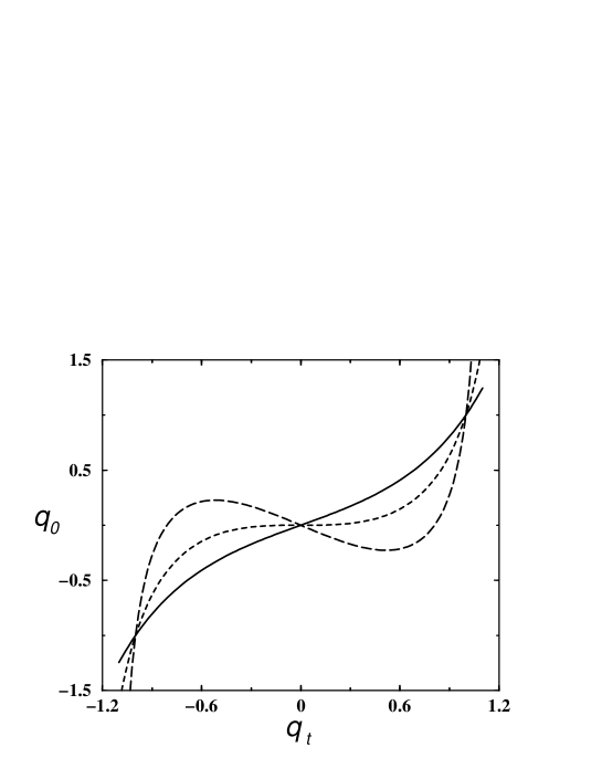
FIG. 2.: $q_{0}(q_{\rm t},\Theta)$ [Eq. (37)] for $\Theta=2.0$ (solid line), $\Theta=\pi$ (short-dashed line), and $\Theta=4.5$ (long-dashed line). For $\Theta<\pi$ this function is one-to-one. For $\Theta>\pi$ and $|q_{0}|$ sufficiently small there are three (or more) real values of $q_{\rm t}$ corresponding to a given $q_{0}$.

FIG. 3.: $-iq_{0}(\xi,\Theta)$ [Eq. (44)] for $\Theta=2.0$ (solid line), $\Theta=2.5$ (short-dashed line), and $\Theta=\pi$ (long-dashed line).

FIG. 4.: $\rho(0,0)$ vs. $\Theta$ for $g=0.3$. Usual (dashed line) and improved (solid line) semiclassical approximation.

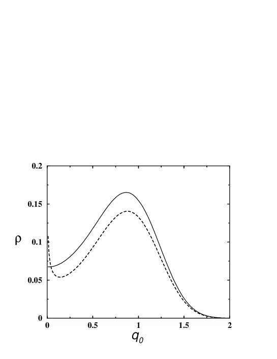
FIG. 5.: $\rho(q_{0},q_{0})$ vs. $q_{0}$ for $\Theta=\pi$. Usual (dashed line) and improved (solid line) semiclassical approximation.

FIG. 6.: $\rho(q_{0},q_{0})$ vs. $q_{0}$ for $\Theta=5.0$ and $g=0.3$. Usual (dashed line) and improved (solid line) semiclassical approximation.

FIG. 7.: $q_{\rm t}$ vs. $q_{0}$ for $\Theta=5.0$. If $|q_{0}|<q_{*}=0.3332\ldots$, there are three real solutions to Eq. (37) (solid lines); the upper curve corresponds to the global minimum, the lower one to the local minimum, and the one in the middle to a one-saddle. At the caustic the last two coalesce, and reappear at the other side of the caustic (i.e., $|q_{0}|>q_{*}$) as a pair of complex conjugate solutions. Their real and imaginary parts are represented by the long-dashed and short-dashed lines, respectively.

- [1] R. P. Feynman, Statistical Mechanics (Addison-Wesley, New York, 1972).
- [2] L. S. Schulman, Techniques and Applications of Path Integration (John Wiley, New York, 1981).
- [3] H. Kleinert, Path Integrals in Quantum Mechanics, Statistics and Polymer Physics (World Scientific, Singapore, 1995).
- [4] C. A. A. de Carvalho, R. M. Cavalcanti, E. S. Fraga, and S. E. Jorás, Ann. Phys. (N.Y.) 273, 146 (1999) [quant-ph/9810045].
- [5] C. A. A. de Carvalho, R. M. Cavalcanti, E. S. Fraga, and S. E. Jorás, Phys. Rev. E 61, 6392 (2000) [quant-ph/9910055].
- [6] W. H. Miller, Science 233, 171 (1986).
- [7] C. A. A. de Carvalho and R. M. Cavalcanti, Braz. J. Phys. 27, 373 (1997) [quant-ph/9803049].
- [8] M. V. Berry, Adv. Phys. 25, 1 (1976).
- [9] H. Trinkaus and F. Drepper, J. Phys. A: Math. Gen. 10, L11 (1977).
- [10] M. V. Berry, J. F. Nye, and F. J. Wright, Phil. Trans. R. Soc. Lond. A 291, 453 (1979).
- [11] M. Berry, in Physics of Defects, Les Houches Session XXXV (1980), edited by R. Balian, M. Kléman, and J.-P. Poirier (North-Holland, Amsterdam, 1981).
- [12] M. V. Berry and C. Upstill, in Progress in Optics XVIII, edited by E. Wolf (North-Holland, Amsterdam, 1980).
- [13] R. Balian and C. Bloch, Ann. Phys. (N.Y.) 63, 592 (1971); 85, 514 (1974).
- [14] R. Thom, Structural Stability and Morphogenesis (Benjamin, Reading, MA, 1975).
- [15] T. Poston and I. N. Stewart, Catastrophe Theory and its Applications (Pitman, London, 1978).
- [16] G. Dangelmayr and W. Veit, Ann. Phys. (N.Y.) 118, 108 (1979).
- [17] I. Affleck, Phys. Rev. Lett. 46, 388 (1981).
- [18] E. M. Chudnovsky, Phys. Rev. A 46, 8011 (1992).
- [19] U. Weiss, Quantum Dissipative Systems (World Scientific, Singapore, 1993).
- [20] J. Ankerhold and H. Grabert, Physica A 188, 568 (1992).
- [21] F. J. Weiper, J. Ankerhold, and H. Grabert, Physica A 223, 193 (1996) [quant-ph/9512015].
- [22] B. J. Harrington, Phys. Rev. D 18, 2982 (1978).
- [23] L. Dolan and J. Kiskis, Phys. Rev. D 20, 505 (1979).
- [24] For a review, see A. Cuccoli, R. Giachetti, V. Tognetti, R. Vaia, and P. Verrucchi, J. Phys.: Condensed Matter 7, 7891 (1995). See also Ref. [3].
- [25] M. Bachmann, H. Kleinert, and A. Pelster, Phys. Rev. A 60, 3429 (1999) [quant-ph/9812063].
- [26] I. S. Gradshteyn and I. M. Ryzhik, Table of Integrals, Series, and Products (Academic Press, New York, 1965).
- [27] P. F. Byrd and M. D. Friedman, Handbook of Elliptic Integrals for Engineers and Physicists (Springer-Verlag, Berlin, 1954).
- [28] J. L. Richard and A. Rouet, Nucl. Phys. B 185, 47 (1981).
- [29] S. Coleman, Aspects of Symmetry (Cambridge University Press, Cambridge, 1985), Ch. 7.
- [30] G. C. Rossi and M. Testa, Ann. Phys. (N.Y.) 148, 144 (1983).