Pseudo-forces in quantum mechanics

Abstract

Dynamical evolution is described as a parallel section on an infinite dimensional Hilbert bundle over the base manifold of all frames of reference. The parallel section is defined by an operator-valued connection whose components are the generators of the relativity group acting on the base manifold. In the case of Galilean transformations we show that the property that the curvature for the fundamental connection must be zero is just the Heisenberg equations of motion and the canonical commutation relation in geometric language. We then consider linear and circular accelerating frames and show that pseudo-forces must appear naturally in the Hamiltonian.

I Introduction

Evolution of a state vector in quantum mechanics can be viewed as a kind of parallel transport asorey . There have been suggestions to use the geometric language of vector bundles and parallel transport in various situations in quantum mechanicsprugo ; drech ; gau ; sarda ; bozo . These ideas are natural in the discussion of the geometric or the Berry phasegeo .

Despite these attempts to “geometrize” quantum mechanics there seems to be no common agreement in these approaches about the base space, or the structure group, let alone the connection or the curvature. Moreover it is not clear whether the extra mathematical machinary is justified by a new or clearer physical insight.

In this paper we give the physical reason why the bundle viewpoint is natural in quantum mechanics and illustrate it with application to accelerated frames.

If a physical system is observed in various frames of reference, the states described by them as vectors in their individual Hilbert spaces will form a section in a vector bundle with the Hilbert space as the standard fiber and the set of all frames of reference as the base manifold. There is no canonical identification of the fibers and we need a “connection”, a notion of covariant derivative or that of parallel transport.

We make use of the principle of relativity (all frames of reference are equally suitable for description) to provide the notion of parallelism and make the following assumption: States described by different frames of reference form a parallel section.

As each observer can apply an overall unitary operator on his Hilbert space and still obtain an equivalent description, we see that the structure group should be the group of all unitary operators on the Hilbert spacebohm . Thus there is an underlying “gauge freedom” which can be used to transform the natural parallel sections into constant sections and do away with the need to use all Hilbert spaces at once. This is the case in standard quantum mechanics where a single Hilbert space is used by all observers.

In this paper we develop our geometric picture and explicitly consider the case where Galilean group is the underlying relativity group. We find that Heisenberg equations of motion and the canonical commutation relation are contained in a single condition: that the fundamental connection is flat or that its curvature is zero.

Next we apply the geometric construction to accelerated frames and show that pseudo-force terms appear as expected. In the case of linearly accelerated frames we get a linear “gravitational” potential implying that equivalence principle must hold in quantum mechanics. In contrast, in the conventional formalism equivalence principle is obtained by an artificial time dependent phase transformation of the wavefunction. In the case of rotating frames we show that both centrifugal and coriolis forces show up in the Hamiltonian. It is satisfactory to see that the coriolis force does not correspond to a potential because it does no work, being perpendicular to velocity, but naturally appears as a connection term added to the canonical momentum, much like the magnetic force. We are thus able to show that fibre bundles are the natural language in which to discuss quantum mechanical effects of gravity.

II Geometric setting

II.1 The bundle

Consider a quantum mechanical system described by observers in different frames of reference. We assume that the set of all frames of reference forms a differentiable manifold. This is physically reasonable because frames of reference are related by symmetry transformations which form a group. This means that the frames can be labelled by coordinates $x$ on the group manifold. A state of the system is described by a vector $\phi(x)$ in a Hilbert space ${\mathcal{H}}_{x}$ associated with the observer $x$. We, thus, have the ingredients of a vector bundlechern . The base is a manifold $M$ with coordinates $x$ and a Hilbert space at each point. To every possible state of the system is associated a section or a mapping $x\rightarrow\phi(x)$ where $\phi(x)$ is the vector describing the state of the system by observer $x$. We assume there exist unitary operators $U(y,x)$ which connect the states $\phi(y)=U(y,x)\phi(x)$. These operators must satisfy consistency conditions

$$U(z,y)U(y,x)=U(z,x);\qquad U(x,x)=1$$

We must note that there is no canonical way of choosing states $\phi(x)$ to describe the system in the Hilbert space ${\mathcal{H}}_{x}$. If we were to apply a unitary operator to all vectors $\phi(x),\ \psi(x)$ etc. in ${\mathcal{H}}_{x}$, the resulting states are equally well suited to describe the system provided the observables acting in ${\mathcal{H}}_{x}$ are similarly changed. In other words, we assume the structure or gauge group acting on the fiber to be the group of all unitary operators.

II.2 The Connection

Let us choose a complete orthonormal set $\phi_{\alpha}$ in the Hilbert space of some fixed observer, say at $x=0$, $\phi_{\alpha}\equiv\phi_{\alpha}(0)$. The sets ${\phi_{\alpha}(x)}=U(x,0)\phi_{\alpha}(0)$ then are complete orthonormal sets in all the other spaces ${\mathcal{H}}_{x}$. Any arbitrary section $\psi(x)$ can then be written as

$$\psi(x)=\sum_{\alpha}c_{\alpha}(x)\phi_{\alpha}(x)$$

where $c_{\alpha}(x)$ are the complex coefficients of expansion. Let $\Gamma$ be the set of all sections. They can be added pointwise.

$$\big{(}\psi_{1}+\psi_{2}\big{)}(x)=\psi_{1}(x)+\psi_{2}(x)$$

and multiplied with smooth functions

$$(c\psi)(x)=c(x)\psi(x)$$

Let $\Lambda\otimes\Gamma$ be the tensor product of the space $\Lambda$ of all 1-forms on the base $M$ and $\Gamma$. A connection on this bundle is a mapping $D:\Gamma\rightarrow\Lambda\otimes\Gamma$ such that

$$D(\psi_{1}+\psi_{2}) = D\psi_{1}+D\psi_{2}\qquad{\rm and}$$

$$D(c\psi) = cD\psi+dc.\psi$$

$(4)$

If $\phi_{n}(x)$ is a basis in $\Gamma$ we can express $D(\phi_{n})$ in terms of the basis $dx^{\mu}\otimes\phi_{m}$ in $\Lambda\otimes\Gamma$ as

$$(D\phi_{n})(x)=\phi_{m}(x)\Gamma_{\mu mn}dx^{\mu}$$

where coefficients $\Gamma_{\mu mn}(x)$ are the Christoffel symbols with respect to the basis $dx^{\mu}\otimes\phi_{m}$. We write this equation as

$$(D\phi_{n})(x)=\phi_{m}\omega^{\phi}_{mn}(x)$$

where the complex matrix $\omega_{mn}$ can be obtained by taking inner product with $\phi_{m}$ in Eq.(5).

$$\omega^{\phi}_{mn}=\big{(}\phi_{m},D\phi_{n}\big{)}$$

This matrix of one-forms is called the connection matrix. We require $D$ to satisfy Leibniz rule

$$D(\phi,\psi)=(D\phi,\psi)+(\phi,D\psi)=d(\phi,\psi)$$

which when applied to $\delta_{mn}=(\phi_{m},\phi_{n})$ shows that $\omega^{\phi}$ is an anti-hermitian matrix.

Under a change of basis

$$\chi_{n}(x)=U(x)\phi_{n}(x)$$

we have

$$\chi_{n}(x) = \phi_{m}(x)\big{(}\phi_{m}(x),U(x)\phi_{n}(x)\big{)}$$

$$= \phi_{m}(x)U_{mn}(x)$$

$(10)$

Thus, omitting the base point $x$ for simplicity of notation

$$(D\chi_{n})(x) = D\big{(}\phi_{s}U_{sn}\big{)}$$

$$= \phi_{r}\omega^{\phi}_{rs}U_{sn}+\phi_{s}dU_{sn}$$

$$= \chi_{m}\omega^{\chi}_{mn}=\phi_{r}U_{rm}\omega^{\chi}_{mn}$$

$(11)$

Or,

$$\omega^{\chi}_{mn}=U^{-1}_{mr}\omega^{\phi}_{rs}U_{sn}+U^{-1}_{mr}dU_{rn}$$

Omitting matrix indices, we have

$$\omega^{\chi}=U^{-1}\omega^{\phi}U+U^{-1}dU$$

The curvature 2-form for the connection is given by

$$\Omega^{\phi}=d\omega^{\phi}+\omega^{\phi}\wedge\omega^{\phi}$$

which transforms as

$$\Omega^{\chi}=U^{-1}\Omega^{\phi}U$$

One may also note the Bianchi identity

$$d\Omega=\Omega\wedge\omega-\omega\wedge\Omega$$

III Parallel section and the fundamental connection

We now make the fundamental assumption that a system observed by different observers is represented by parallel sections. Let $\phi_{m}(x)$ be a family of parallel sections, that is

$$(D\phi)(x)=0,\qquad\qquad{\rm for\,\,all}\ m$$

This implies

$$\omega^{\phi}_{mn}(x)=0$$

everywhere.

We shall now see how does the connection matrix look like with respect to the basis of constant sections. The advantage of using constant sections is that one can give up the bundle picture altogether and identify all Hilbert spaces together to work in one common space. The constant section physically means that the state is represented by the same constant vector by all observers. This is the most general definition of the Heisenberg picture.

To get constant sections we use the fact that parallel sections are constructed by applying transformation $U(x,0)$ on $\phi(0)$ for all $x$.

$$\phi_{m}(x)=U(x,0)\phi_{m}(0)=U(x)\phi_{m}(0)$$

We can choose $\phi_{m}(0)$ as the new basis

$$\chi_{m}(x)\equiv\phi_{m}(0) = U_{x}^{-1}\phi_{m}(x)$$

$$= \phi_{r}(x)\big{(}\phi_{r}(x),U^{-1}(x)\phi_{m}(x)\big{)}$$

$$= \phi_{r}(x)U^{-1}_{rm}$$

$(20)$

Then

$$\omega^{\chi}=UdU^{-1}$$

which, as expected, is pure gauge.

IV Galilean frames

Let us consider a particle of mass $m$ in one space dimension. We use units where $c=\hbar=1$. We consider the basis of sharp momentum states $|k\rangle$ such that

$$P|k\rangle=k|k\rangle$$

and

$$\langle k^{\prime}|k\rangle=\delta(k-k^{\prime})$$

The time and space translations are given by the operators $U_{\tau}$ and $U_{\zeta}$ respectively,

$$U_{\tau}|k\rangle=e^{-iH\tau}|k\rangle=e^{-i{{k^{2}}\over{2m}}}|k\rangle$$

$$U_{\zeta}|k\rangle=e^{iP\zeta}|k\rangle=e^{ik\zeta}|k\rangle$$

The boosts act as

$$U_{\eta}|k\rangle=|k-m\eta\rangle$$

given by

$$U_{\eta}=e^{-iK\eta}$$

where $K$ is the boost generator. The lie algebra of the Galilean group is

$$[P,H]=0,\hskip 28.45274pt[K,H]=iP$$

$$[K,P]=imI$$

The algebra is not closed. This is because unitary representation of the Galilean group in $\mathcal{H}$ is projective. The position operator $X$ is related to $K$ali as

$$K=mX$$

and it acts on the states $|k\rangle$ as

$$\langle k|X=i{{\partial}\over{\partial k}}\langle k|$$

Parallel sections can be constructed using $U_{\tau}$, $U_{\zeta}$ and $U_{\eta}$ in a variety of ways. We choose the following convention which corresponds to the transformations

$$x^{\prime} = x-\eta t-\zeta$$

$$t^{\prime} = t-\tau$$

$$v^{\prime} = v-\eta$$

$(31)$

between frame $S$ and $S^{\prime}$. If we take the standard frame at $x=0,\ t=0,\ v=0$ then

$$\phi(x^{\prime},t^{\prime},v^{\prime}) = \phi(-\zeta,-\tau,-\eta)$$

$$= U_{\tau}U_{\zeta}U_{\eta}\phi(0,0,0)$$

$(32)$

We rename coordinates

$$\phi(x,t,v)=U_{-t}U_{-x}U_{-v}\phi(0,0,0)$$

and get for the basis of constant sections

$$\omega^{\chi} = U_{-t}U_{-x}U_{-v}d\Big{(}U_{-t}U_{-x}U_{-v}\Big{)}^{-1}$$

$$= i\Big{(}-Hdt+Pdx+X(t)mdv-mxdv\Big{)}$$

$(34)$

The curvature is zero, as it should be for a pure gauge connection. But it is worth seeing explicitly.

$$\Omega^{\chi}=d\omega+\omega\wedge\omega=0$$

This implies the following equations

$$i{\dot{P}}=[P,H]$$

$$i{\dot{X}}=[X,H]$$

$$[X,P]=i$$

Equations (34) and (35) are just the Heisenberg equations of motion for operators $P$ and $X$ while the third is the canonical commutation relation for $X$ and $P$.

One may argue that these equations are just reproductions of the algebra. Indeed the algebra is used in the calculation of the curvature. What is new is that in this differential geometric language all the information is contained in a single zero curvature equation.

V Accelerated frames and pseudo forces

Acceleration implies changing from one Galilean frame to another after every infinitesimal amount of time. This can be seen as a curve on the base manifold parametrized by time. We assume that an observer in the accelerating frame uses the same Hilbert space to describe a physical system as the observer at the base manifold point with which it coincides at each instant $t$. Moreover they assign the same state to the systembell .

V.1 Linearly accelerated frame and equivalence principle

The question of whether the principle of equivalence in classical mechanics also holds in quantum mechanics was discussed by C.J. Eliezer and P.G. Leacheliezer . They studied the transformation of the Schrödinger equation under a change from an inertial frame of reference $S$ to a uniformly accelerating one $S^{\prime}$. Their argument goes as follows. Let

$$x^{\prime}=x+{{1}\over{2}}gt^{2},\qquad t^{\prime}=t$$

be the change of coordinates to an accelerated frame. Then he equivalence principle holds provided the phase of the wavefunction of the system is redefined by a time dependent expression. This means that the Schrödinger equation in the frame $S$

$$i{{d\psi}\over{dt}}=-{{1}\over{2m}}\nabla^{2}\psi$$

transforms to the equation for a particle moving in a uniform field

$$i{{d\psi^{\prime}}\over{dt^{\prime}}}=-{{1}\over{2m}}\nabla^{\prime 2}\psi^{\prime}-mgx^{\prime}\psi^{\prime}$$

with the redefinition of the phase of $\psi$ given by

$$\psi^{\prime}(x^{\prime})=exp\Big{(}{{img}\over{\hbar}}(x^{\prime}t^{\prime}-{{1}\over{6}}gt^{\prime 3}\Big{)}\psi(x)$$

The phase factor has been chosen precisely to obtain equivalence principle. There is no explanation put forward for this factor.

In our formalism we find that the equivalence principle must hold in quantum mechanics in a straightforward manner. There is no need for any other condition such as the redefinition of the wavefunction by a time-dependent phase factor, like the one seen above.

Consider an observer in a linearly accelerated frame of reference. The linear acceleration corresponds to a curve on the base manifold parametrized by $t$ and given by

$$x={{1}\over{2}}gt^{2}$$

$$v=gt$$

The parallel section is again specified by

$$|t,x,v;k\rangle\equiv U_{v}U_{x}U_{t}|k\rangle$$

The rate of change of the vector along the curve should give the Hamiltonian for the accelerated observer. We get

$$i{{d}\over{dt}}|t,x,v;k\rangle = i{{d}\over{dt}}\Big{(}U_{t}U_{x}U_{v}|k\rangle\Big{)}$$

$$= \Big{(}{{(k-mv)^{2}}\over{2m}}+(k-mv)t{{dv}\over{dt}}-(k-mv){{dx}\over{dt}}$$

$$-mx{{dv}\over{dt}}-mgx-i{{dv}\over{dt}}{{\partial}\over{\partial v}}\Big{)}|t,x,v;k\rangle$$

$$= \Big{(}{{P(v)^{2}}\over{2m}}-X(x)mg\Big{)}|t,x,v;k\rangle$$

$(46)$

where $P(v)=k-mv$ and $X(x)=X+x$. Thus, the system “sees” an extra potential $X(x)mg$ which is the expected linear “gravitational” potential term. This is manifestation of the equivalence principle in quantum mechanics.

The validity of the equivalence principle in the quantum regime has been experimentally tested in some beautiful experiments done with neutron interferencecow .

V.2 Rotating frame, coriolis and centrifugal forces

Consider a frame of reference $S^{\prime}$ which is rotating with constant angular velocity $\omega$ and radius $r$ about the origin of coordinates on the $xy$ plane of a frame $S$. The two frames are related as follows: we wait for time $t$, translate by ${{\bf r}}$ direction, rotate by angle $\theta=\omega t$ and finally give a boost in the $y^{\prime}$ direction by velocity $v$.

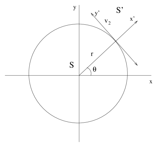
Figure 1: $S^{\prime}$ is a frame which is rotating with angular velocity $\omega$ about origin of frame $S$ with radius $r$.

The parallel section is given by

$$U = U_{v}U_{\theta}U_{{\bf r}}U_{t}$$

$$= e^{-i{\vec{X}}_{2}mv}e^{iJ\theta}e^{iP.{{\bf r}}}e^{-i{{P^{2}}\over{2m}}t}$$

$(47)$

where $J=X_{1}P_{2}-X_{2}P_{1}$ is the angular momentum operator. The curve on the base manifold parametrized by $t$ is

$${{\bf r}} = (r\,{\rm cos}\,\theta,r\,{\rm sin}\,\theta)$$

$${{\bf v}} = (-r\omega\,{\rm sin}\,\theta,r\omega\,{\rm cos}\,\theta)$$

$(48)$

The Hamiltonian $H$ as seen by an observer in the rotating frame is given by the rate of change of the vectors specified along the curve on the base manifold.

$$H = i{{dU}\over{dt}}U^{-1}$$

$$= {{1}\over{2m}}\Big{(}P_{1}^{2}+(P_{2}+m\omega r)^{2}\Big{)}-\omega r(P_{2}+m\omega r)$$

$$-\omega\big{(}J+m\omega r\big{)}$$

$(49)$

or

$$H = {{1}\over{2m}}\Big{(}(P_{1}+m\omega X_{2})^{2}+(P_{2}-m\omega X_{1})^{2}\Big{)}$$

$$-{{1}\over{2}}m\omega^{2}\big{(}(X_{1}+r)^{2}+X_{2}^{2}\big{)}$$

$(50)$

Thus the expected centrifugal and coriolis forces appear in the Hamiltonian. Since coriolis force does no work it cannot appear as an explicit potential term. Rather it appears as a connection in the canonical momentum.

VI Discussion

The bundle viewpoint is hinted in Dirac’s work as early as 1932. In a most influential paper The Lagrangian in quantum mechanicsdirac Dirac puts forth the following argument: Let $q(t)$ be a complete set of commuting observables in the Heisenberg picture. The set of eigenvalues $q^{\prime}$ at each $t$ forms a manifold $M$ giving rise to “spacetime” $B\equiv M\times T$ where $T$ represents the time axis.

Evolution is determined by the moving basis $\langle q^{\prime},t|$ at each $(q^{\prime},t)$. This can be interpreted as a section from the base $B$ into a Hilbert space. Let $c:\tau\rightarrow(q^{\prime}(\tau),t(\tau))$ be a curve in $B$. Then the change of basis vectors $\langle q^{\prime},t|$ is given by

$$-i{\partial\over{\partial q^{\prime}}}\langle q^{\prime},t|=\langle q^{\prime},t|\,P(t)$$

$$i{\partial\over{\partial t}}\langle q^{\prime},t|=\langle q^{\prime},t|\,H$$

where $P(t)=e^{iHt}P(0)e^{-iHt}$

Thus the change of a basis vector along the curve is

$$d\langle q^{\prime},t|=i\langle q^{\prime},t|\,dS$$

$$dS=P(t)dq^{\prime}-Hdt$$

Thus in the bundle formalism Dirac’s Lagrangian can be seen as an operator -valued 1-form on the Hilbert vector bundle whose base manifold is spanned by the eigenvalues $q^{\prime}$ of a complete set of commuting operators $q(t)$ specified at all times and the standard fibre is Hilbert space. The components of this 1-form are just the Hamiltonian and momentum operators. If the section $(q^{\prime},t)\to\langle q^{\prime},t|$ is assumed to be parallel then evolution can be seen as parallel transport. This is the theme on which our present work is based.

Asorey et al. asorey consider a Hilbert bundle with positive time axis ${\mathcal{R}}^{+}$ as the base manifold. Another viewpoint is that of Prugoveckiprugo and Drechsler and Tuckeydrech whose bundle is the associated vector bundle for the principle bundle with Poincare group as structure group over spacetime base manifold. The Hilbert space considered by them is the space of square integrable functions over phase space of space coordinates and the mass hyperboloid ($p^{2}=m^{2},\ p_{0}>0$). This approach allows them to consider parallel transport over curved spaces with possible applications to quantum gravity.

Dirk Graudenzgau also has a Hilbert bundle with spacetime base. Our approach agrees with that of Graudenz in that description of a physical system is always description by one observer. Yet another construction is given by G. Sardanashvilysarda who consider a $C^{*}$-algebra at each point of the time axis ${\mathcal{R}}$.

Our geometric construction is different from others in the literature. For us the base manifold consists of all frames of reference. This means actually having a group of symmetry transformations as the base manifold with a frame of reference associated with each point on it. We have considered the case of Galilean group which makes the application specific to quantum mechanics.

Our objective here is to present a new geometric viewpoint from which implies the validity of the equivalence principle in quantum mechanics. We have demonstrated this both for linearly accelerating and rotating frames.

References

- (1) M.Asorey, J.F.Carinena and M.Paramio, J. Math. Phys. 23, 8(1982)
- (2) E. Prugovecki, Class. Quant. Grav., 13, 1007 (1996)
- (3) W. Drechsler and P. A. Tuckey, Class. Quant. Grav., 13, 611(1996)
-
(4)
Dirk Graudenz,CERN-TH.7516/84
Dirk Graudenz, hep-th/9604180 - (5) G. Sardanashvily, quant-ph/0004050
- (6) Bozhidar Iliev, J. Phys. A 31, 1297(1998)
- (7) A.Shapere and F.Wilczek (eds.), Geometric Phases in Physics, World Scientific, Singapore, 1989.
-
(8)
It has been shown by
A.Bohm, B. Kendrick, M.E. Loewe and L.J. Boya, J. Math. Phys., 33, 3 (1992),
that the structure group also appears in the discussion of gauge theory of the slow motion part of a molecule in the exact case. - (9) S.S.Chern, Chen and Lam, Lectures on Differential Geometry, World Scientific, 1999.
- (10) S.T. Ali, J.P. Antoine and J.P. Gazeau, Annals of Physics, 222, 1, 1993.
-
(11)
J.S. Bell and J.M. Leinaas, Nucl. Phys.B 284, 488-508, (1987)
(Section 2, page 490) - (12) C.J. Eliezer and P.G. Leach, Am. J. Phys., 45, 1218 (1977)
-
(13)
R. Cotella, A.W. Overhauser and S.A. Werner, Phys. Rev.
Lett. 34, 1472-1474 (1975)
Ulrich Bonse and Thomas Wroblewski, Phys. Rev. Lett. 51, 1401-1404 (1983)
Daniel M. Greenberger and A.W. Overhauser, Rev. Mod. Phys., 51, 43-78 (1979) - (14) P.A.M. Dirac, Phys. Z. Sowjetunion, Vol.3, 1 (1933).