An optical kaleidoscope using a single atom

Abstract

A new method to track the motion of a single particle in the field of a high-finesse optical resonator is described. It exploits near-degenerate higher-order Gaussian cavity modes, whose symmetry is broken by the phase shift on the light induced by the particle. Observation of the spatial intensity distribution behind the cavity allows direct determination of the particle’s position with approximately wavelength accuracy. This is demonstrated by generating a realistic atomic trajectory using a semiclassical simulation including friction and diffusion and comparing it to the reconstructed path. The path reconstruction itself requires no knowledge about the forces on the particle.

In a variety of pioneering experiments in the past few years[1, 2, 3] it has been demonstrated and widely exploited that a single near-resonant atom can significantly influence the field dynamics in a microscopic high-finesse optical resonator. Vice versa, the light field also influences the motion of a cold atom, which leads to an intricate dynamical interplay of atomic motion and field dynamics [4, 5]. As a striking example, trapping of a single atom in the field of a single photon has become feasible[6, 7]. This was experimentally substantiated by analyzing the characteristics of the measured output field. The time variation of the transmitted intensity shows very good agreement with theoretical simulations[8] of the confined three-dimensional motion of the atom in the cavity light field including friction and diffusion [9, 10, 11]. Carrying this analysis further it was even possible to associate piecewise reconstructed trajectories with recorded time-dependent intensity curves[7, 12], utilizing the knowledge of the near-conservative potential. However, the reconstruction was possible only for atoms with sufficiently large and conserved angular momentum around the cavity axis and can only be done up to an overall angle and the direction of rotation. The reason was that only a single cavity mode, the TEM₀₀ mode, was used. Consequently, only a single spatial degree of freedom of the atom could be extracted directly from a measurement of the transmitted field.

In this letter, we propose a new method to obtain two-dimensional information on the atom’s position. We consider higher-order frequency-degenerate transversal modes. Typical examples are the Hermite-Gaussian (HG) or the Laguerre-Gaussian (LG) modes, which show in the transverse plane a rectangular matrix of intensity minima and maxima or a pattern of concentric rings, respectively. In such a configuration, the atom can redistribute photons from one mode to the other. Moreover, it induces mode frequency shifts and losses strongly dependent on the atomic position. In particular, the symmetry of the intracavity field determined by the cavity and pump geometry will be perturbed and characteristic optical patterns containing information on the atomic position appear. The effect reminds of a toy-kaleidoscope in which small objects in a symmetric arrangement of mirrors create beautiful patterns. Our technique yields much more information on the atomic position and motion as compared to the single-mode case, and allows to extract the atomic position directly from a field measurement.

To treat this problem quantitatively we generalize previous semiclassical models of dynamical cavity QED in the strong-coupling regime to include finite sets of nearly degenerate eigenmodes. For a weakly saturated atom we derive a coupled set of equations for the mode amplitudes and the atomic center-of-mass motion. To be specific, let us consider a single two–level atom with transition frequency $\omega_{a}$ and line width $\Gamma$ (half width at half maximum) moving inside a high-finesse optical resonator with transversal LG eigenmodes $u_{pm}({\bf{r}})$, where $p$ is the radial mode index and $m$ is the azimuthal mode index [13],

$$u_{pm}(\rho,\theta,z) = C_{pm}\cos(kz)e^{-\frac{\rho^{2}}{{\mathrm{w}_{0}}^{2}}+im\theta}$$ (2)

$$\times(-1)^{p}(\frac{\rho\sqrt{2}}{{\mathrm{w}_{0}}})^{|m|}L_{p}^{|m|}(\frac{\sqrt{2}\rho^{2}}{{\mathrm{w}_{0}}^{2}}),$$

where $L_{n}^{\alpha}$ is the generalized Laguerre polynomial. The normalisation parameters, $C_{pm}$, are chosen such that $\int|u_{pm}(\rho,\theta,z)|^{2}{\rm d}V=d{\mathrm{w}_{0}}^{2}\pi/4=V_{00}$ (the TEM₀₀ mode volume), where ${\mathrm{w}_{0}}$ is the cavity waist and $d$ the cavity length. At each spatial point the local atom-mode couplings are $g_{pm}({\bf{r}})=g_{0}u_{pm}({\bf{r}})$, where $g_{0}$ is the maximum coupling of the TEM₀₀ mode. For simplicity, we assume that the mirrors are ideally spherical and have a uniform coating. Then, all these modes have a common eigenfrequency $\omega$ and field decay rate $\kappa$. However, the model can be extended to incorporate non-degenerate modes in a straightforward manner. The cavity is also assumed short compared to the Rayleigh length of the mode so that the wavefronts are approximately plane with $z$-dependence $\cos(2\pi z/\lambda)$. The resonator is externally driven by a coherent pump field of frequency $\omega_{p}$ which pumps the modes with strengths $\eta_{pm}$. Assuming low atomic saturation, we can adiabatically eliminate the internal atomic dynamics and treat the atom as a linearly polarizable particle, which induces a spatially dependent phase shift and loss. In the semiclassical limit[14], where we consider the center-of-mass motion of the atom classically, we can derive the following set of coupled differential equations for the mode amplitudes $\alpha_{k}(t)$, the atomic position ${\bf{r}}_{a}(t)$ and momentum ${\bf{p}}_{a}(t)$:

$$\dot{{\bf{r}}}_{a} = \frac{{\bf{p}}_{a}}{M},$$ (3)

$$\dot{{\bf{p}}}_{a} = -U_{0}\sum_{m,n}\nabla(u_{pm}u_{pn}^{*})\alpha_{pm}\alpha_{pn}^{*}$$ (5)

$$+i\gamma\sum_{m,n}(u_{pm}\nabla u^{*}_{pn}-u^{*}_{pn}\nabla u_{pm})\alpha_{pm}\alpha^{*}_{pn}+\chi,$$

$$\dot{\alpha}_{pm} = \eta_{pm}+(i\Delta-\kappa)\alpha_{pm}$$ (7)

$$-(iU_{0}+\gamma)u_{pm}\sum_{n}u^{*}_{pn}\alpha_{pn}+\xi_{pm}.$$

Here, $M$ is the atomic mass, $U_{0}=g_{0}^{2}/(\omega_{p}-\omega_{a})$ is the single-photon optical light shift, $\gamma=\Gamma g_{0}^{2}/(\omega_{p}-\omega_{a})^{2}$ the spontaneous emission rate for a single-photon field, $\Delta=\omega_{p}-\omega$ the cavity-pump detuning, and $\chi$ and $\xi_{pm}$ are Gaussian random variables which model momentum and cavity field fluctuations, respectively.

As an example, we consider an atom at rest at a given position ${\bf{r}}_{a}$ coupled to the three degenerate cavity modes with $(p,m)=(1,0),(0,-2),(0,2)$. It is then possible to solve equations (7) for the mean stationary field amplitudes $\alpha_{pm}^{\mbox{stat}}({\bf{r}}_{a})$, which in a parametric way depend on the atomic position. We get:

$$\alpha_{pm}^{\mbox{stat}}=\frac{\eta_{pm}^{*}}{i\Delta-\kappa}+\frac{iU_{0}+\gamma}{i\Delta-\kappa}u_{pm}^{*}({\bf{r}}_{a}){\cal E}_{0}({\bf{r}}_{a}),$$ (8)

where ${\cal E}_{0}$ is the electric field at the position of the atom,

$${\cal E}_{0}({\bf{r}}_{a})=\frac{\sum_{p,m}u_{pm}({\bf{r}}_{a})\eta_{pm}^{*}}{(i\Delta-\kappa)-(iU_{0}+\gamma)\sum_{p,m}|u_{pm}({\bf{r}}_{a})|^{2}}.$$ (9)

Note that the set of mode amplitudes $u_{pm}({\bf{r}}_{a})$ at the position of the atom may be written as a vector, which can then be rotated into the form $(u_{\rm eff}({\bf{r}}_{a}),0,0)$. Since any linear combination of the modes can be considered as a mode as well, the atom-field dynamics for an atom at rest thus reduces to the case of a single mode $u_{\rm eff}$. This allows to derive simple analytical expressions for the steady state. For a moving atom, this approach must be generalized, but still helps to find analytical expressions for friction and diffusion coefficients for the atomic motion [15].

Figure 1 shows the steady state field intensities for the empty cavity and for two different atomic positions. For the chosen parameters (rubidium atoms, $(g_{0},\Gamma,\kappa)=2\pi\times(16,3,1.5)\,$MHz, $(\eta_{10},\eta_{0-2},\eta_{02})=2\pi\times(6.4,0,0)\,$MHz, $\Delta=-2\pi\times 2.25\,$MHz and $\omega_{p}-\omega_{a}=-2\pi\times 114\,$MHz, leading to $U_{0}=\Delta$, $\gamma=2\pi\times 60\,$kHz) the atom distributes photons between the cavity modes and changes their relative phases in such a way that a local maximum of the total field intensity is created near the position of the atom. By a change of the detuning between the pump laser, the cavity modes, and the atomic transition, a local minimum can also be achieved. Figure 1 shows the effect of the atom position on the shape and overall intensity of the stationary field distribution.

This dependence of the cavity field on the atomic position suggests that measuring the cavity output field distribution yields ample information on the atomic motion. In fact, it can be shown that the functions $\alpha_{pm}^{\mbox{stat}}({\bf{r}}_{a})$ can be inverted almost everywhere to yield the atomic position in three dimensions. Of course one is limited by the common symmetries of all modes. For instance, for the system considered in Fig. 1, a $180^{\circ}$ rotation around the cavity axis forms a symmetry operation. Hence, the reconstruction of the atomic position from the cavity field will always yield two equivalent positions. Other symmetry operations are a shift of $\lambda/2$ in direction of the cavity axis and a reflection at the nodes or antinodes of the standing wave. Another limitation is that an atom cannot be detected close to the (transversal) nodes of the pumped mode (see Fig. 1a). However, it is possible to determine directly from the photodetector signals whether the atomic position can be obtained or not: reconstruction is possible if the transmission signal with an atom differs from the signal of an empty cavity. Also, the nodal areas are small and one is free to alternate rapidly between different pump geometries. Alternatively, one can change the pump geometry online when the atom approaches the nodal area of the pumped mode.

Although in principle a full three-dimensional atomic trajectory can be reconstructed, the method encounters some complications. The longitudinal motion is in general too fast to be resolved experimentally. This amounts to replacing the coupling constant $g_{0}^{2}$ by its longitudinally averaged value. A two-dimensional reconstruction still works in this case, even if the precise factor by which the coupling is reduced is unknown. Second, a single atom must redistribute enough photons among the cavity modes. This requires values of $U_{0}$ of the order of the cavity decay rate $\kappa$ and hence the strong-coupling regime of cavity QED. Third, our arguments above are based on a stationary cavity field. For an atom moving in the $xy$ plane, we thus have to assume that the cavity field follows the atomic motion adiabatically. This implies slow atomic motion and not too large optical forces in this plane, which together with the constraint of strong coupling is tantamount to relatively low intracavity photon numbers. Fourth, in an actual experiment the exact intracavity photon number can only be deduced from the number of photons emitted by the cavity. The measured cavity output is subject to statistical fluctuations (shot noise), which become significant in the few photon limit. This limits the accuracy to which the cavity field, and therefore the atomic position, can be known.

In the following we will demonstrate with a sample trajectory that all of these conditions can be met simultaneously and that the numerical reconstruction of the atomic path is possible using existing high-finesse optical resonators [6, 7]. For simplicity we will assume a quasi two-dimensional situation where the atom is trapped in the longitudinal cavity direction at an antinode ($z=0$) of the standing wave during the full interaction time.

In a first step we create a sample trajectory for a single atom traversing the resonator by integrating the stochastic equations of motion (7) for given initial atomic position and velocity. This procedure includes all reactive and dissipative optical forces which the cavity field imposes on the atom [14], the back-action of the atom on the cavity field, as well as the momentum and cavity field diffusion. A resulting trajectory is depicted by the solid curve in Fig. 2. The atom enters the resonator from below. By chance, the atom encircles the cavity axis a few times before it is ejected again.

The generated trajectory allows us to simulate a realistic cavity output signal. We assume an arrangement of 16 photodetectors at the cavity output port each counting the numbers of photons detected in equally sized sectors extending from the axis to the edges of the cavity and covering an angle of 22.5 degrees. Due to the symmetry of the system, the signals from opposing detectors can be added without loss of information. To reduce the shot noise, we integrate the measured photon flux at each detector over a time interval of 100 cavity decay times $1/\kappa$. In Fig. 3 we plot the simulated photon flux for two out of the eight pairs of photodetectors.

We can use the generated time-dependent field pattern to numerically reconstruct the particular atomic trajectory. This involves several steps. First, for each time step we determine the atomic position by a least-square comparison with a list of precalculated detector outputs corresponding to the steady-state field distribution $\alpha_{pm}^{\mbox{stat}}({\bf{r}}_{a})$ of any atomic position on a discrete spatial grid. Because of the twofold spatial symmetry, we always obtain two equivalent points in that way. Hence, from a chosen initial point we have selected the one point out of these two that forms a continuous curve as a function of time. The spatial points obtained in that way are indicated by the crosses in Fig. 2. The initial position of the atom is usually known in experiments where laser-cooled atoms are injected into the cavity. For the pump geometry chosen here, there is a dark ring where the atom does not couple to the pumped mode. Close to this ring, the reconstruction is difficult. As mentioned before, there are ways around this problem, but here the corresponding crosses are simply left out.

According to the temporal noise of the measured photon fluxes (Fig. 3), the reconstructed atomic positions show a certain spatial spread. Since for the given parameters the stochastic forces in Eqs. (7) are much smaller than the Hamiltonian forces, we finally fit a smooth curve to this discrete set of data. The resulting reconstructed trajectory is shown by the dashed curve in Fig. 2. Note that the curve rotated by $180^{\circ}$ forms a completely equivalent solution to the problem. Comparing the reconstructed with the original trajectory we note that for the depicted area close to the cavity axis the reconstruction works well with an accuracy which is of the order of an optical wavelength.

The proposed detector arrangement might be constructed by segment mirrors imaging onto an array of single-photon counting detectors. Probably more practically is direct imaging on a high-sensitive high-speed camera. The construction of a suited cavity will be challenging. Scatter, misalignment and deformation of the high-reflectivity mirrors must be kept to a minimum to prevent breaking of the cylindrical symmetry, which could lift the frequency degeneracy of the modes by a too large amount.

It is interesting to note that positive or negative values for $m$ in the Laguerre-Gaussian modes correspond to actual left- and right-handed rotation of the light around the cavity axis. Hence, there is a striking similarity between Fabry-Perot cavities sustaining higher-order Laguerre-Gaussian modes and ring cavities. Similar dynamics as predicted in Ref. [16] can therefore be expected in the system proposed here.

An extension of the idea presented here is to use a cavity where modes with different longitudinal mode index are degenerate. In that case, one can choose a combination of modes with opposite parity to break the $180^{\circ}$ rotation symmetry. An example is a LG mode with even $m$ degenerate with another one with odd $m$. In the extreme case of a confocal cavity, this will lead to a single field maximum near the position of the atom.

In conclusion, we have shown how a high-finesse microcavity can be used as a real-time single-particle detector with high spatial resolution. In contrast to conventional single-atom detection schemes, the cavity works as a phase-contrast microscope enhanced by the inherent multi-path interference of the high-finesse cavity. The method does not rely on fluorescence and, hence, can also work for particles without a closed optical transition. In contrast to the single-mode case, the information in the field pattern of sufficiently high-order modes should also allow one to spatially resolve several particles. It can be expected that the scheme presented here will first be demonstrated with single atoms in presently available high-finesse cavities, but applications extend beyond this system. The method should, in principle, also be applicable to large (bio)molecules in vacuum or even in pure watery solution.

P. H. and H. R. acknowledge support by the Austrian Science Foundation FWF (project P13435-TPH).

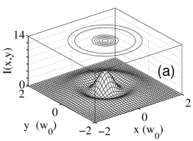
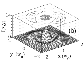
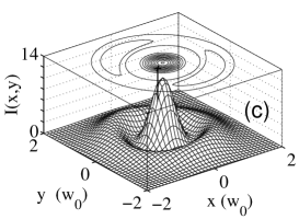
FIG. 1.: Transversal spatial intensity pattern (arbitrary units) of the stationary cavity field for the empty cavity (a) and two atomic positions indicated by the thick vertical line and a cross (b), (c).

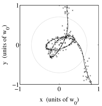
FIG. 2.: Central part of Fig. 1(a) with the simulated atomic trajectory (solid curve), reconstructed atomic positions (crosses), and fitted atomic path (dashed curve). The atom enters with a velocity of $12\,$cm/s and the total trajectory takes $~{}5300\,\kappa^{-1}=0.56\,$ms. The dashed circle indicates the dark ring of the pumped cavity mode $u_{10}$. The waist of the TEM₀₀ mode is ${\mathrm{w}_{0}}=29\,\mu$m.

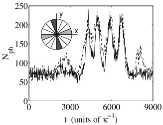
FIG. 3.: Simulated photon flux (number of photons $N_{\rm ph}$ per 100 $\kappa^{-1}$) measured at two out of 8 photodetector pairs as a function of time (units of $\kappa^{-1}$). The inset depicts the arrangement of the detectors on the cavity output, shaded areas correspond to the plotted curves.

REFERENCES

- [1] H. Mabuchi, Q.A. Turchette, M.S. Chapman, H.J. and Kimble, 1996, Opt. Lett. 21, 1393 (1996).
- [2] P. Münstermann, T. Fischer, P.W.H. Pinkse, and G. Rempe, Opt. Commun. 159, 63 (1999).
- [3] J.J. Childs, K. An, M.S. Otteson, R.R. Dasari, and M.S. Feld, Phys. Rev. Lett. 77, 2901 (1996).
- [4] C.J. Hood, M.S. Chapman, T.W. Lynn, and H.J. Kimble, Phys. Rev. Lett. 80, 4157 (1998).
- [5] P. Münstermann, T. Fischer, P. Maunz, P.W.H. Pinkse, and G. Rempe, Phys. Rev. Lett. 82, 3791 (1999).
- [6] P.W.H. Pinkse, T. Fischer, P. Maunz, and G. Rempe, Nature 404, 365 (2000).
- [7] C.J. Hood, T.W. Lynn, A.C. Doherty, A.S. Parkins, and H.J. Kimble, Science 287, 1447 (2000).
- [8] A.C. Doherty, A.S. Parkins, S.M. Tan, and D.F. Walls, Phys. Rev. A 56, 833 (1997).
- [9] P. Horak, G. Hechenblaikner, K.M. Gheri, H. Stecher, and H. Ritsch, Phys. Rev. Lett. 79, 4974 (1997).
- [10] P.W.H. Pinkse, T. Fischer, P. Maunz, T. Puppe, and G. Rempe, J. Mod. Opt. 47, 2769 (2000).
- [11] M. Gangl and H. Ritsch, Eur. Phys. J. D 8, 29 (2000).
- [12] A.C. Doherty et. al, Phys. Rev. A 63, 013401 (2000).
- [13] A.E. Siegman, Lasers (University science books, Mill Valley, CA 1986).
- [14] P. Domokos, P. Horak, and H. Ritsch, J. Phys. B: At. Mol. Opt. Phys. 34, 187 (2001).
- [15] T. Fischer, P. Maunz, T. Puppe, P.W.H. Pinkse, and G. Rempe, submitted to New Journal of Physics. Here, the Langevin equations are solved for an ensemble of atoms by defining an effective polarization, which has great similarities with the effective mode approach.
- [16] M. Gangl and H. Ritsch, Phys. Rev. A 61, 043405 (2000).