Information capacity formula of quantum optical channels

Abstract

The applications of the general formulae of channel capacity developed in the quantum information theory to evaluation of information transmission capacity of optical channel are interesting subjects. In this review paper, we will point out that the formulation based on only classical-quantum channel mapping model may be inadequate when one takes into account a power constraint for noisy channel. To define the power constraint well, we should explicitly consider how quantum states are conveyed through a transmission channel. Basing on such consideration, we calculate a capacity formula for an attenuated noisy optical channel with genreral Gaussian state input; this gives certain progress beyond the example in our former paper [13].

1 Introduction

During about twenty years, the information theory for quantum channel has been devised[3]. It is called quantum information theory. The most fundamental result in it is the formula of channel capacity, which might be an interesting subject for optical communication issue; if one wants to know the ultimate capability of information transmission, one has to know the channel capacity.

Here we introduce short survey of a channel model and its capacity theory [9]. Let ${\{|\alpha_{m}\rangle}\}$, $m=1,2$ be binary letter states, whose state overlap is $\kappa=\langle\alpha_{1}|\alpha_{2}\rangle$. By $n$-th extension, we choose $M$ codeword states $\{|\psi_{1}\rangle,\cdots,|\psi_{M}\rangle\}$ $(M\leq 2^{n})$ from the $2^{n}$ possible sequences of length $n$, and use them with respective a priori probabilities $\{\pi_{1},\cdots,\pi_{M}\}$, where $|\psi_{i}\rangle=|\alpha_{m_{1}}(i)\rangle\otimes|\alpha_{m_{2}}(i)\rangle\ |\otimes\alpha_{m_{3}}(i)\rangle\otimes\cdots\otimes|\alpha_{m_{n}}(i)\rangle$. We can regard a codeword state as one signal state. Since the codeword states are linearly independent, they span the $M$ dimensional Hilbert space. Then the optimization problem of quantum decoding is reduced to the detection problem for $M$-ary no coded quantum signals. The above statements are the definition of the quantum coding and decoding for Shannon information. Here, the decoding means abstract representation of optical receivers, which are described by so called positive operator valued measure(POVM). The decoding processes can be classified into two classes in general. One of them is decoding based on ”individual separate measurement”. It means that each bit of codeword is measured and a received codeword is decoded by the data processing based on $n$ measured variables. However, the super additivity is not allowed by decoding based on the individual separate measurement[18]. This decoding operator (or detection operator) is described as follows:

$$\hat{\mit\Pi}_{i}=\otimes_{k=1}^{n}\hat{{\mit\Pi}_{k}}^{(i)}$$ (1)

where $\hat{{\mit\Pi}_{k}}^{(i)}$ is the optimum detection operator for letter states. The other is decoding based on entangled or collective measurement, which is called ”entangled decoding”. In the latter case, the codeword state is regarded as single state and a set of $M$ detection operators for $M$-ary no coded quantum states is applied to decide them. Therefore, one can obtain only $M$ values of detection for $M$ codewords in the decoding process. In this model, there is a bound for capacity, so called Holevo bound. His general formula involves also the mixed state case. The detailed discussion is given in the later sections. Then, for pure state case, Hausladen, Jozsa, Schumacher, Westmoreland, and Wooters[8] proved that the Holevo bound for the information transmission by pure state is really channel capacity. That is, the zero error channel capacity $C$ is defined by $\lim_{n\to\infty}{C_{n}}/{n}$ and it is given by the maximization of von Neumann entropy with respect to a priori probability for an ensemble of signal states.

Recently, Holevo[11], and Schumacher-Westmoreland[19] proved that the Holevo bound is also the channel capacity in the general case (mixed state case). Finally, Holevo gave the formula for the continuous alphabet[12]. As a result, the capability of information transmission increases by design of coding and decoding for $n$th extension. Then a fundamental property, super additivity of channel capacity by extended codes, ${C}_{n}$+ ${C}_{m}$ $\leq$ ${C}_{n+m}$, was found.

In this paper, we survey the general scheme of the theory of channel capacity, and show how to apply them to optical communication process. Finally, the general capacity formula for optical channel with energy loss and back ground noise is given, which corresponds to Shannon formula: $C=\log(1+{S}/{N})$.

In Section 2, we present a quantum model of optical communication, ”attenuated noisy channel”. In preparation for calculating the capacity of such a channel, we survey the results about the channel coding theorem in Sections 3 and 4: In Section 3, we consider the ”classical-quantum channel model”, which is a generalization of attenuated noisy channel, and give the general formula of its capacity. To calculate the channel capacity, we need to solve an optimization problem included in the general capacity formula (see the formulation (28)). In Section 4 we calculate the channel capacity for quantum Gaussian channel, solving the optimization problem. Modifying this calculation, we obtain the capacity of the attenuated noisy channel in Section 5, where the formulae (55) and (58) are main results of this paper. In Section 6 we discuss a discretization of quantum continuous channel.

2 Quantum Model of Optical Communication

We start with presenting a quantum model of optical communication, which is the main subject of our interest. In our model, one mode Bosonic states, which the transmitter outputs, are conveyed through an attenuation channel with classical noise. We can formulate this model as follows.
(i) transmitted Bosonic states
Let ${\hat{a}}$ be an annihilation operator on a Hilbert space ${\cal{H}}$. We take as an input alphabet ${\cal{A}}$ the complex plane ${\mathbb{C}}$ or nonnegative integer ${\mathbb{Z}}_{0}^{+}$, and assume that the transmitter sends a Bosonic state $\tilde{\rho}(\mu)$ corresponding to a letter $\mu\in{\cal{A}}$. In particular our concern is concentrated on two examples: (a) $\tilde{\rho}(\mu)={\cal{D}}(\mu)\tilde{\rho(0)}$ with a squeezed state $\tilde{\rho}(0)$ and the unitary displacement operator ${\cal{D}}(\mu)=\exp(\mu{\hat{a}}^{\dagger}-\bar{\mu}{\hat{a}})$, (b) $\tilde{\rho}(n)$ are number states $|n{\rangle}{\langle}n|$ ($n\in{\mathbb{Z}}_{0}^{+}$).
(ii) linear attenuator with classical noise
The linear attenuator with coefficient $k\leq 1$ and Gaussian noise with variance $N_{c}$ is described by the transformation

$${\hat{a}}^{\prime}=k{\hat{a}}+\sqrt{1-k^{2}}{\hat{a}}_{0}+\xi,$$ (2)

in the Heisenberg picture. In the equation (2), ${\hat{a}}_{0}$ is an annihilation operator in another mode in the Hilbert space ${\cal{H}}_{0}$ of an ”environment” and $\xi$ is a complex random variable with zero mean and variance $N_{c}$. We assume that the environment is initially in the vacuum state. We denote by $\Gamma$ the corresponding transformation of states in the Shrödinger picture: ${\rm Tr}\tilde{\rho}(\mu){\hat{a}}^{\prime}={\rm Tr}\Gamma[\tilde{\rho}(\mu)]{\hat{a}}$.
(iii) detection process
Consider the code of size $M$, $\{u_{1},u_{2},...,u_{M}\}$, consisting of codewords of length $n$, $u_{i}=(\mu_{i_{1}},...,\mu_{i_{n}})$, where $\mu_{i_{j}}$ is selected from the continuous input alphabet ${\cal{A}}={\mathbb{C}}$ or the discrete one ${\cal{A}}={\mathbb{Z}}_{0}^{+}$. Then the codeword $u_{i}$ is related to a product state $\rho(\mu_{i_{1}})\otimes\cdots\otimes\rho(\mu_{i_{n}})\in{\cal{H}}\otimes\cdots\otimes{\cal{H}}\equiv{\cal{H}}^{\otimes n}$, where $\rho(\mu_{i_{j}})=T[\tilde{\rho}(\mu_{i_{j}})]$. This correspondence gives a channel mapping stated in Section 3. A detection process is given by a detection operator ${\hat{\Pi}}_{i}$, which is a positive operator-valued measure (POVM) on ${\cal{H}}^{\otimes n}$ [10] defined as

$$\begin{split}{\hat{\Pi}}_{i}&\geq 0,\quad\forall i,\\ \sum_{i=1}^{M}{\hat{\Pi}}_{i}&={\hat{I}}.\end{split}$$ (3)

The POVM represents a measurement process and decision for a signal to be $u_{i}$ based on the measurement result. Using POVM, the conditional probability of the output $u_{j}$, given the input was $u_{i}$, is obtained as,

$$P(u_{j}|u_{i})={\rm Tr}\rho_{u_{i}}{\hat{\Pi}}_{j}.$$ (4)

How to define information quantities for such a channel, is shown in the next section using a more general formulation.

3 Coding Theorem of Quantum Channel for Shannon Information

In this section we survey the coding theorem for classical-quantum channels, where Shannon information is conveyed by quantum states.

3.1 Finite alphabet system

3.1.1 Holevo-Schumacher-Westmoreland theorem

Let ${\cal{H}}$ be a Hilbert space. The classical-quantum channel (coding channel) with discrete alphabet ${\cal{A}}=\{1,..,a\}$ consists of the mapping $i\to\rho_{i}$ from the input alphabet to the set of density operators in ${\cal{H}}$. The input is described by an a priori probability distribution $\pi=\{\pi_{i}\}$ on ${\cal{A}}$. A quantum detection process (decoding channel) is described by POVM ${\hat{\Pi}}=\{{\hat{\Pi}}_{j}\}$ on ${\cal{H}}$. Like Eq. (4) the conditional probability of the output $j$, given the input was $i$, is obtained as,

$$P(j|i)={\rm Tr}\rho_{i}{\hat{\Pi}}_{j},$$ (5)

and the Shannon’s mutual information is given by

$$I_{1}(\pi,{\hat{\Pi}})=\sum_{j}\sum_{i}\pi_{i}P(j|i)\log\left(\frac{P(j|i)}{\sum_{k}\pi_{k}P(j|k)}\right).$$ (6)

Moreover let us consider the product channel in the tensor product Hilbert space ${\cal{H}}^{\otimes n}={\cal{H}}\otimes\cdots\otimes{\cal{H}}$ with the input alphabet ${\cal{A}}^{n}$ consisting of words $u=(i_{1},...,i_{n})$ of length $n$, with density operator

$$\rho_{u}=\rho_{i_{1}}\otimes\cdots\otimes\rho_{i_{n}}.$$ (7)

If $\pi$ is a probability distribution on ${\cal{A}}^{n}$ and ${\hat{\Pi}}$ is a POVM on ${\cal{H}}^{\otimes n}$, we can define the information quantity $I_{n}(\pi,{\hat{\Pi}})$ by a formula similar to (6). Now let us define

$$C_{n}=\sup_{\pi,{\hat{\Pi}}}I_{n}(\pi,{\hat{\Pi}}).$$ (8)

Then we have the property of super additivity

$$C_{n}+C_{m}\leq C_{n+m},$$ (9)

and hence the following limit exists:

$$C=\lim_{n\to\infty}C_{n}/n.$$ (10)

This limit gives a definition of capacity of the initial channel. Here it should be emphasized that in the definition of this quantity we employ an entangled measurement. The use of such measurement causes the superadditivity, which is characteristic of quantum system. In contrast, in a semi classical case, we consider individual separate measurement of the form (1), and carry out error correction based on data processing of measured value. Such a detection strategy never produces the super additivity, but only achieves $C_{1}$.

Using the von Neumann entropy, which is defined as $H(\rho)=-{\rm Tr}\rho\log\rho$ for a density operator $\rho$, we can obtain a simple formula of the capacity:
Theorem[11, 19]:
The capacity of arbitrary signal states $\rho_{i}$, having finite entropy $H(\rho_{i})$, is given by

$$C=\lim_{n\to\infty}{C_{n}}/{n}=\max_{\pi}\Delta H(\pi),$$ (11)

where

$$\Delta H(\pi)=H\left(\sum_{i\in{\cal{A}}}\pi_{i}\rho_{i}\right)-\sum_{i\in{\cal{A}}}\pi_{i}H(\rho_{i}).$$ (12)

In general the computation of the quantity $C$ is very difficult, but, fortunately, if the signal states $\rho_{i}$ have a certain symmetry, the analytical solution can be obtained: Let us consider signal states given as

$$\rho_{i}={\hat{V}}^{i-1}\rho_{1}{\hat{V}}^{\dagger i-1}$$ (13)

where ${\hat{V}}^{\dagger}{\hat{V}}={\hat{V}}{\hat{V}}^{\dagger}={\hat{V}}^{M}={\hat{I}}$. Then it is shown [15] that the capacity is achieved by a uniform distribution on a priori probabilities. In particular, when $\rho_{1}$ is a pure state represented as $\rho_{1}=|\psi{\rangle}{\langle}\psi|$, the capacity is calculated as,

$$C=-\sum_{j=1}^{M}\lambda_{j}\log\lambda_{j},$$ (14)

where $\lambda_{j}$ is

$$\lambda_{j}=\frac{1}{M}\sum_{k=1}^{M}{\langle}\psi|{\hat{V}}^{k-1}|\psi{\rangle}\exp\left(-\frac{2j(k-1)\pi i}{M}\right).$$ (15)

3.1.2 $C_{1}$ and Accessible information

As described in Sec. 3.1.1, most essential property of quantum theory for capacity is the super additivity. For research of coding scheme achieving the capacity, we have to clarify properties of the super additivity. As a first step, we consider accessible information, which is defined to be

$$I_{{\rm ac},n}(\pi)=\sup_{{\hat{\Pi}}}I_{n}(\pi,{\hat{\Pi}}),$$ (16)

for fixed a priori distribution $\pi$. A necessary condition for quantum measurement ${\hat{\Pi}}$ achieving the accessible information ${I_{{\rm ac},1}}(\pi)$ was given as follows[10]:

$$\hat{\mit\Pi}_{i}\left({\cal{F}}_{i}-{\cal{F}}_{j}\right)\hat{\mit\Pi}_{j}=0,\forall i,j,$$ (17)

where

$${\cal{F}}_{j}=\displaystyle\sum_{l}\pi_{l}\log\left[\frac{P(j|l)}{\sum_{k}\pi_{k}P(j|k)}\right]{\rho}_{l}.$$ (18)

Since the above equation provides only a necessary condition for detection operators, we cannot, in general, solve the problems. From another point of view, Davies proved theorems[4] of conditions for optimum detection operators which give accessible information. His theorems require that one has to take into account a number of detection operator $J$ corresponding to a size of detection scheme to get an accessible information. That is, $d\leq J\leq d^{2}$, where $d$ is the dimension of Hilbert space of letter states.

Now let us consider $C_{1}$. Although to derive $C_{1}$ is very difficult, Davies’s theorems play an important role to search it actually. Based on these theories, Levitin[16], Fuchs and Caves[5], and Fuchs and Peres[6] gave some examples of $C_{1}$ as almost final result, and they clarified an importance of this problem in a quantum information theory. On the other hand, Ban[2] and Osaki[17] proved that if the signal states are group covariant, then the square root measurements or minimax solutions in quantum detection theory satisfy Holevo’s necessary condition for information criterion, and finally Osaki numerically[17] and Ban analytically [1] derived ${C}_{\rm 1}$ of the binary pure states taking all parameters into account. The final result: ${C}_{\rm 1}$ is so simple as follows:

$$C_{1}=1-H(P_{\rm e}(2))$$ (19)

where $H(P_{\rm e}(2))$ is entropy for error probability, $P_{\rm e}(2)$ is the minimum error probability in the detection problem for binary states,

$$P_{\rm e}(2)=\left[1-(1-{\kappa}^{2})^{\frac{1}{2}}\right]/2$$ (20)

where $\kappa$ is the inner product between two pure states.

Let us turn the problem into the system with linearly dependent state. If there are three states in $2$ dimensional Hilbert space, then they are linearly dependent. When they have equal angle each other, the channel capacity of letter states is $C_{1}=0.6698$, where $C_{1}$ is given by $\pi_{1}=\pi_{2}=1/2$, and $\pi_{3}=0$. However, we have no exact solution for other cases.

3.2 Infinite alphabet system

Let us turn to the infinite alphabet system; we present a general formula of capacity for a quantum continuous channel according to [13].

Take as the input alphabet ${{\cal{A}}}$ an arbitrary Borel subset in a finite-dimensional Euclidean space ${\cal E}$. Then the quantum continuous channel is described by a weakly continuous mapping ${\mu\to\rho(\mu)}$ from the input alphabet ${\cal{A}}$ to the set of density operators in ${\cal H}$, where we assume that the states $\rho(\mu)$ have a finite von Neumann entropy $H(\rho(\mu))=-{\rm Tr}\rho(\mu)\log\rho(\mu)$, moreover

$$\sum_{\mu\in{\cal{A}}}H(\rho(\mu))<\infty.$$

Like the discrete case, we treat the product memoryless channel in the Hilbert space ${\cal H}^{\otimes n}={\cal H}\otimes\cdots\otimes{\cal H}$ ($n$ copies). Then the signal $u_{i}=(\mu_{i_{1}},...,\mu_{i_{n}})$ is related to a density operator $\rho(\mu_{i_{1}})\otimes\cdots\otimes\rho(\mu_{i_{n}})$. In a similar way as the classical case, we impose the power constraint

$$f(\mu_{i_{1}})+\cdots+f(\mu_{i_{n}})\leq nE$$ (21)

on the signals $u_{i}=(\mu_{i_{1}},...,\mu_{i_{n}})$, where $f$ is a continuous positive function on ${\cal E}$. In particular, we denote by ${\cal{P}}_{1}$ a set of probability distributions $\pi$ on ${\cal{A}}$ satisfying

$$\int_{{\cal{A}}}f(x)\pi(dx)\leq E.$$ (22)

Without the constraint we cannot obtain anything but meaningless results, that is, arbitrary high transmission rates can be achieved with arbitrary low error probability with essentially no coding.

The theory of capacity of continuous channel was established by Holevo. Let us sketch the outline of the theory according to [12]. We consider discretization of the channel by taking a priori distributions with discrete support

$$\pi(d\mu)=\sum_{i}\pi_{i}\delta_{\mu_{i}}(d\mu),$$ (23)

where $\{\mu_{i}\}$ is arbitrary countable collection of points and

$$\delta_{\mu}(B)\equiv\left\{\begin{array}[]{rl}1&\mbox{if $\mu\in B$,}\\ 0&\mbox{if $\mu\notin B$.}\end{array}\right.$$ (26)

Then the capacity $C$ is defined as follows.

$$C = \sup_{\pi\in{\cal{P}}^{\prime}_{1}}\Delta H(\pi),$$ (27a)

$$\Delta H(\pi) \equiv H\left(\int_{\cal{A}}\rho_{x}\pi(dx)\right)-\int_{\cal{A}}H(\rho_{x})\pi(dx),$$ (27b)

where ${\cal{P}}^{\prime}_{1}$ is a set of a priori distributions with discrete support satisfying input constraint (22). Holevo proved [12] that all rates below the channel capacity are achievable, and that under some assumptions the channel capacity $C$ is equal to

$$\sup_{\pi\in{\cal{P}}_{1}}\Delta H(\pi).$$ (28)

So far we have described the theory for channel capacity. As a result, the channel coding theorem has been proved for quantum channel which corresponds to quantum measurement process. This theorem provides interesting results. That is, the channel capacity is exactly equal to the Holevo bound which is defined without the model of quantum measurement process, while the capacity is defined for channel model of the quantum measurement process as described in the equations (6)-(10). So if one wants to calculate only channel capacity, one needs not the physical channel model. In other word, the capacity is given only by the ensemble of prepared states or density operators in front of the measurement. Thus, sometimes, in mathematical papers the channel is defined by a mapping from classical alphabet to quantum states or density operators; it is called classical-quantum channel. However, in order to evaluate the capacity of the attenuated noisy channel described in Section 2, we should consider a slightly different channel model, which is described in the next subsection.

3.3 Channel model for describing a power constraint

@

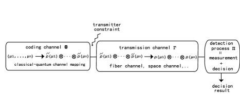
Figure 1: channel model with transmitter constraint

We present channel model consisting of three components as shown in Figure 1:
(1) coding channel: In the coding channel codewords $(\mu_{1},...,\mu_{n})$ are related to quantum states $\tilde{\rho}(\mu_{1})\otimes\cdots\otimes\tilde{\rho}(\mu_{n})$ respectively. Thus the coding channel is described as classical-quantum channel mapping $\Phi:(\mu_{1},...,\mu_{n})\to\tilde{\rho}(\mu_{1})\otimes\cdots\otimes\tilde{\rho}(\mu_{n})$.
(2) transmission channel: Through the transmission channel quantum states $\tilde{\rho}(\mu_{1})\otimes\cdots\otimes\tilde{\rho}(\mu_{n})$ are conveyed, and transformed to quantum states $\rho(\mu_{1})\otimes\cdots\otimes\rho(\mu_{n})$ respectively. Thus the transmission channel is described by completely positive map $\Gamma:\tilde{\rho}(\mu_{1})\otimes\cdots\otimes\tilde{\rho}(\mu_{n})\to\rho(\mu_{1})\otimes\cdots\otimes\rho(\mu_{n})$. (3) detection process.
This model gives a generalization of the attenuated noisy channel.

When we consider only (discrete) channel without power constraint, we can apply the general capacity formula (11) directly to the above model by regarding $\bar{\Phi}^{(n)}=\Gamma^{(n)}\circ\Phi^{(n)}$ as the classical-quantum channel mapping. On the other hand, for a continuous channel, we should consider a constraint on the average power of signals $\tilde{\rho}(\mu_{1})\otimes\cdots\otimes\tilde{\rho}(\mu_{n})$ that the transmitter outputs; such a constraint is called transmitter constraint in the following. Then we have no way to describe the power constraint function $f$ in (21) and (22) by using only $\bar{\Phi}^{(n)}$. In other words we cannot formulate the optimization in (27) only by $\bar{\Phi}^{(0)}$, while we can represent $\Delta H(\pi)$ as a function of $\pi$ and $\bar{\Phi}^{(0)}$. This is the reason why we should explicitly distinguish coding channel $\Phi^{(n)}$ from transmission channel $\Gamma^{(n)}$ in our model. Although use of the power constraint on the energy of input signals $(\mu_{1},...,\mu_{n})$ does not produce such a problem, it is not suitable for evaluation of the capacity of the attenuated noisy channel.

In the attenuated noisy channel the transmission map $\Gamma^{(n)}$ is parametrized by $k$ and $N_{c}$, which are defined in Section 2. As a result, its channel capacity is given as a function of $k$, $N_{c}$, and $\Phi^{(0)}(0)=\tilde{\rho}(0)$ in Section 5.

4 Channel Capacity Formula for quantum Gaussian States

In this section we calcuate the channel capacity, based on the channel mapping model $\mu\to\rho(\mu)$ with input constraint according to [13]. In particular we treat the case where $\rho(\mu)$ are quantum Gaussaian states. The results will be applied to calculation of capacity for the attenuated noisy channel in Section 5.

4.1 Quantum Gaussian state

We introduce a Gaussian density operator, which is defined to be a density operator with a characteristic function of the form,

$${{\rm Tr}}\rho V(z)=\exp\left[im^{t}z-\frac{1}{2}z^{t}\alpha z\right],$$ (29)

where $z$ is a column $2s$-dimensional vector $[x_{1},...,x_{s};y_{1},..,y_{s}]^{t}$ and

$$V(z)=\exp i\sum_{j=1}^{s}[x_{j}q_{j}+y_{j}p_{j}].$$ (30)

In the characteristic function, $m$ is a column $2s$-vector and $\alpha$ is a real symmetric $2s\times 2s$ matrix, satisfying

$$m={\rm Tr}\rho R,\quad\alpha-\frac{i}{2}\Delta={\rm Tr}R\rho R^{t},$$ (31)

where $R=[q_{1},..,q_{s};p_{1},...,p_{s}]$ and

$$\Delta=\left[\begin{array}[]{cc}O&\hbar I\\ -\hbar I&O\end{array}\right],$$ (32)

with identity matrix $I$ and zero matrix $O$.

4.2 Calculation of capacity

The mapping from classical parameter to quantum Gaussian state is, in mathematical paper, called quantum Gaussian channel, which forms an important class of the continuous classical-quantum channel described in Section 3.2. Holevo and coworkers provided the general formula of capacity of this channel. Take as input alphabet ${\cal{A}}$ the complex plane ${\mathbb{C}}$, and as the density operator $\rho(0)$ a Gaussian one with mean $0$. Then the quantum Gaussian channel is described by the mapping $\mu\to\rho(\mu)$, where $\rho(\mu)={\cal{D}}(\mu)\rho(0)$ with the displacement operator ${\cal{D}}(\mu)$. Here we restrict ourselves to the case where we impose the input constraint. The input constraint is given by putting $f(\mu)=\hbar\omega|\mu|^{2}$ in (21) and (22).

To carry out calculation of capacity for such a channel, the following two properties of quantum Gaussian channel are essentially used [13]:
(i) the optimum a priori distribution $\pi$ in (27) is Gaussian, and the mixture $\rho_{\pi}=\int\rho(\mu)\pi(d\mu)$ is Gaussian again. Let correlation matrices of a priori distribution $\pi$ and density operators $\rho$ and $\rho_{\pi}$ be $\beta$, $\alpha$ and $\gamma$ respectively. Then the relation $\gamma=\alpha+\beta$ holds between them.
(ii) von Neumann entropy of Gaussian density operator $\rho$ with a correlation matrix $\alpha$ is calculated as

$$H(\rho)=\frac{1}{2}{\rm Sp}G(-(\Delta^{-1}\alpha)^{2}),$$ (33)

where $G(x^{2})=(x+1/2)\log(x+1/2)-(x-1/2)\log(x-1/2)$. In particular, for one mode Gaussian state the von Neumann entropy is given by

$$H(\rho)=G\left(\frac{\alpha^{qq}\alpha^{pp}-(\alpha^{qp})^{2}}{\hbar^{2}}\right).$$ (34)

Thus the capacity of the quantum Gaussian channel can be written as

$$C=\max_{\beta\in B_{1}}\frac{1}{2}{\rm Sp}G(-[\Delta^{-1}(\alpha+\beta)]^{2})-\frac{1}{2}{\rm Sp}G(-(\Delta^{-1}\alpha)^{2}),$$ (35)

where $B_{1}$ is the convex set of real positive matrices $\beta$, satisfying

$${\rm Sp}\varepsilon\beta\leq E,$$ (36)

where

$$\varepsilon=\left[\begin{array}[]{cc}\varepsilon_{1,1}&O\\ O&1/2I\end{array}\right],$$ (37)

with $\varepsilon_{1,1}={\rm diag}[\omega_{1}^{2}/2,...,\omega_{s}^{2}/2]$, and $s\times s$ zero and identity matrices $O$, $I$.

In the formula (35) the maximization with respect to a priori distribution $\beta$ is left unsolved. Holevo showed [13] the explicit calculation of (35) for one mode quantum Gaussian channel with input constraint. The results are
[A] If the inequality

$$\left[\frac{1}{2}\left(\omega\alpha^{qq}-\frac{\alpha^{pp}}{\omega}\right)\right]^{2}+(\alpha^{qp})^{2}\leq(\frac{E}{\omega})^{2}$$ (38)

holds, then we have

$$\begin{split}C=&G\left(\frac{1}{\hbar^{2}\omega^{2}}\left[E+\frac{1}{2}(\omega^{2}\alpha^{qq}+\alpha^{pp})\right]^{2}\right)\\ &-G\left(\frac{\alpha^{qq}\alpha^{pp}-(\alpha^{qp})^{2}}{\hbar^{2}}\right),\end{split}$$ (39)

where $G(d^{2})=(d+1/2)\log(d+1/2)-(d-1/2)\log(d-1/2)$. By putting $N_{s}=E/\hbar\omega$ and $N={\rm Tr}\rho(0){\hat{a}}^{\dagger}{\hat{a}}=(\omega^{2}\alpha^{qq}+\alpha^{pp})/2\hbar\omega-1/2$, the first term in (39) can be written as

$$(N+N_{s}+1)\log(N+N_{s}+1)-(N+N_{s})\log(N+N_{s}).$$ (40)

When the inequality (38) holds, the mixture $\rho_{\pi}=\int\rho(\mu)\pi(d\mu)$ with the optimum a priori distribution $\pi$ is always equal to the Bose-Einstein distribution with mean number of quanta $N+N_{s}$. Moreover, assuming that $\rho(0)$ is a coherent state, we can also simplify the second term in Eq. (39) and obtain the capacity as

$$\begin{split}C=&(N+N_{s}+1)\log(N+N_{s}+1)-(N+N_{s})\log(N+N_{s})\\ &-(N+1)\log(N+1)+N\log N\\ =&\log\left(1+\frac{N_{s}}{N+1}\right)+(N+N_{s})\log\left(1+\frac{1}{N+N_{s}}\right)\\ &-N\log\left(1+\frac{1}{N}\right).\end{split}$$ (41)

[B] If the inequality (38) does not hold, we have

$$\begin{split}C=&G\left(\frac{1}{\hbar^{2}\omega^{2}}\left\{\left[E+\frac{1}{2}(\omega^{2}\alpha^{qq}+\alpha^{pp})\right]^{2}\right.\right.\\ &\left.\left.-\left[\sqrt{(\omega^{2}\alpha^{qq}-\alpha^{pp})^{2}/4+\omega^{2}(\alpha^{qp})^{2}}-E\right]^{2}\right\}\right)\\ &-G\left(\frac{\alpha^{qq}\alpha^{pp}-(\alpha^{qp})^{2}}{\hbar^{2}}\right).\end{split}$$ (42)

Note that the capacity under output constraint can be obtained by some modifications of the above discussion (see [13]).

5 Application to attenuated noisy channel

The attenuated noisy channel corresponds to optical fiber channel or space channel in optical communication system. In this section, we show the capacity formulae when the communication process has such an attenuated noisy channel.

5.1 Gaussian state

In this subsection we calculate the capacity for the attenuated noisy channel formulated in Sec 2. As a first step, we make some preparations for applying the results in Section 4.2 to this calculation.
(i) construction of the mapping $\mu\to\rho(\mu)$
Since squeezed state is the most general Gaussian state, we treat squeezed state as an example of Gaussian state. The squeezed state $\tilde{\rho}(0)={\cal{S}}(\gamma)|0\rangle$ is described as a pure Gaussian state with correlation matrix

$$\tilde{\alpha}=\left[\begin{array}[]{cc}\tilde{\alpha}^{qq}&\tilde{\alpha}^{qp}\\ \tilde{\alpha}^{qp}&\tilde{\alpha}^{pp}\end{array}\right],$$ (43)

with elements

$$\tilde{\alpha}^{qq} = \frac{\hbar}{2\omega}[\cosh 2\gamma-\sinh 2\gamma\cos\theta]$$ (44)

$$\tilde{\alpha}^{pp} = \frac{\hbar\omega}{2}[\cosh 2\gamma+\sinh 2\gamma\cos\theta]$$ (45)

$$\tilde{\alpha}^{qp} = \frac{\hbar}{2}\sinh 2\gamma\sin\theta.$$ (46)

Then the output state $\rho(\mu)=T[\tilde{\rho}(\mu)]$ has the characteristic function [14]

$${\rm Tr}{\rho}(\mu)V(z)={\rm Tr}\tilde{\rho}(\mu)V(kz)\cdot\exp\left[-\frac{\hbar}{2}\lambda(k,N_{c})z^{t}z\right],$$ (47)

where

$$\lambda(k,N_{c})=\left(\frac{1-k^{2}}{2}+N_{c}\right).$$ (48)

This indicates that $\rho(\mu)={\cal{D}}(k\mu)\rho^{\prime}_{0}{\cal{D}}(k\mu)^{\dagger}$, where $\rho^{\prime}_{0}$ is the Gaussian state with the correlation matrix $\alpha=k^{2}\tilde{\alpha}+\hbar\lambda(k,N_{c}){\hat{I}}$ and the mean 0.
(ii) transmitter constraint
As shown in Section 3.3, instead of input or output constraint given in Section 4.2, we need to introduce a somewhat different constraint for reasonable evaluation of the effect of squeezing. That is, we impose a transmitter constraint

$${\rm Sp}\varepsilon(\tilde{\alpha}+\beta)\leq\hbar\omega\left(N_{tr}+\frac{1}{2}\right),$$ (49)

where $\beta$ is a correlation matrix of a priori probability distribution.

Thus the capacity with the attenuation channel can be written as

$$C=\max_{\beta\in B^{\prime}_{1}}\frac{1}{2}{\rm Sp}G(-[\Delta^{-1}(\alpha+\beta)]^{2})-\frac{1}{2}{\rm Sp}G(-(\Delta^{-1}\alpha)^{2}),$$ (50)

where $B^{\prime}_{1}$ is the convex set of real positive matrices $\beta$, satisfying

$${\rm Sp}\varepsilon\beta\leq k^{2}\left[\hbar\omega\left(N_{tr}+\frac{1}{2}\right)-{\rm Sp}\varepsilon\tilde{\alpha}\right].$$ (51)

We can obtain the explicit formula of the capacity by replacing the energy bound $E$ in (38), (39) and (42) with $k^{2}[\hbar\omega\left(N_{tr}+1/2\right)-{\rm Sp}\varepsilon\tilde{\alpha}]$. In the following we calculate the value of the capacity when $\omega=1$, $\tilde{\alpha}^{qp}=0$, $\tilde{\alpha}^{qq}\geq\tilde{\alpha}^{pp}$ and $\tilde{\alpha}^{qq}\tilde{\alpha}^{pp}=\hbar^{2}/4$ hold. By these substitutions, the inequality (38) becomes

$$\max\{\tilde{\alpha}^{qq},\tilde{\alpha}^{pp}\}\leq\hbar(N_{tr}+1/2),$$ (52)

and we have

$$\begin{split}E+{\rm Sp}\varepsilon\alpha=&\hbar k^{2}(N_{tr}+1/2)+\hbar\lambda(k,N_{c})\\ =&\hbar\left(k^{2}N_{tr}+N_{c}+\frac{1}{2}\right).\end{split}$$ (53)

and

$$\begin{split}\alpha^{qq}\alpha^{pp}=&(k^{2}\tilde{\alpha}^{qq}+\hbar\lambda(k,N_{c}))(k^{2}\tilde{\alpha}^{pp}+\hbar\lambda(k,N_{c}))\\ =&\hbar^{2}[\frac{k^{4}}{4}+k^{2}\lambda(k,N_{c})(2N_{sq}+1)+\lambda(k,N_{c})^{2}]\\ =&\hbar^{2}\left[\left(N_{c}+\frac{1}{2}\right)^{2}+k^{2}N_{sq}[(1-k^{2})+2N_{c}]\right],\end{split}$$ (54)

where $N_{sq}$ is mean number of quanta for a transmitted squeezed state $\tilde{\rho}(0)$, $N_{sq}={\rm Tr}\tilde{\rho}(0){\hat{a}}^{\dagger}{\hat{a}}$. From this the capacity is calculated as follows.
[A] If the inequality (52) holds, we obtain

$$\begin{split}C=&(k^{2}N_{tr}+N_{c}+1)\log(k^{2}N_{tr}+N_{c}+1)\\ &-(k^{2}N_{tr}+N_{c})\log(k^{2}N_{tr}+N_{c})\\ &-G\left(\left[N_{c}+\frac{1}{2}\right]^{2}+k^{2}N_{sq}[(1-k^{2})+2N_{c}]\right).\end{split}$$ (55)

When we transmit coherent states, that is $N_{sq}=0$, the second term in (55) is simplified and the capacity is given by

$$\begin{split}C=&(k^{2}N_{tr}+N_{c}+1)\log(k^{2}N_{tr}+N_{c}+1)\\ &-(k^{2}N_{tr}+N_{c})\log(k^{2}N_{tr}+N_{c})\\ &-(N_{c}+1)\log(N_{c}+1)+N_{c}\log N_{c}.\end{split}$$ (56)

As $G$ in (55) is a monotonously increasing function of $d^{2}$, we can find that the capacity given by (55) is maximized when there is no squeezing $N_{sq}=0$ or when there is no noise and attenuation ($k=1$ and $N_{c}=0$). That is, squeezing necessarily decreases the capacity of attenuated noisy channel.
[B] When the inequality (52) does not hold, using

$$\begin{split}|\alpha^{qq}-\alpha^{pp}|&/2-E\\ =&k^{2}|\tilde{\alpha}^{qq}-\tilde{\alpha}^{pp}|/2-\hbar k^{2}(N_{tr}+1/2)+k^{2}{\rm Sp}\tilde{\alpha}/2\\ =&k^{2}\max\{\tilde{\alpha}^{qq},\tilde{\alpha}^{pp}\}-\hbar k^{2}(N_{tr}+1/2),\end{split}$$ (57)

we obtain

$$\begin{split}C=&G\left(k^{2}[2N_{tr}+1]\left[\lambda(k,N_{c})+k^{2}\frac{\max\{\tilde{\alpha}^{qq},\tilde{\alpha}^{pp}\}}{\hbar}\right]\right.\\ &\quad\quad\quad\left.+\lambda(k,N_{c})^{2}-k^{4}\frac{\max\{\tilde{\alpha}^{qq},\tilde{\alpha}^{pp}\}^{2}}{\hbar^{2}}\right)\\ &-G\left(\left[N_{c}+\frac{1}{2}\right]^{2}+k^{2}N_{sq}[(1-k^{2})+2N_{c}]\right).\end{split}$$ (58)

We would like to call these equations (55) and (58) ”quantum Shannon formula” based on Holevo Theorem, because these correspond to classical Shannon formula $C=\log(1+S/N)$.

@

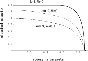
Figure 2: capacity for the attenuated noisy channel

In Figure 2 we present graphs of the capacity with respect to squeezing parameter $\gamma$, when $(k,N_{c})=(1,0)$, $(k,N_{c})=(0.9,0)$ and $(k,N_{c})=(0.9,0.1)$. These graphs show that the capacity for the non-attenuated noiseless channel does not change if squeezing is not too large, while that for attenuated noisy channel is necessarily decreased by any squeezing.

5.2 Number state

If we employ photon number state as the transmitter state, then alphabets are discrete number : $n$. The density operator is described by

$$\rho=\sum_{n}P(n)|n{\rangle}{\langle}n|$$ (59)

In the case of no attenuation process, the maximum entropy is given when

$$P(n)=\frac{1}{1+<n>}\left(\frac{<n>}{1+<n>}\right)^{n}$$ (60)

which is called Bose-Einstein distribution. $<n>$ is average photon number. So the capacity becomes

$$C=\log(1+<n>)+<n>\log(1+\frac{1}{<n>})$$ (61)

For such a photon signal, the channel models of attenuation and amplification processes were discussed by Shimoda, Takahashi, and Townes[20]. The channel model of the noiseless attenuation process is described by binomial distribution as follows:

$$P(n_{y}|n_{x})=\frac{{n_{x}}!}{{n_{y}}!(n_{x}-n_{y})!}k^{n_{y}}(1-k)^{n_{x}-n_{y}}$$ (62)

where $n_{x}$ and $n_{y}$ are input and output photon numbers, respectively. This means that if the input state is certain number state $|n_{x}{\rangle}{\langle}n_{x}|$, then the output is described by

$$\rho_{n_{x}}=\sum_{n_{y}}\frac{{n_{x}}!}{{n_{y}}!(n_{x}-n_{y})!}k^{n_{y}}(1-k)^{n_{x}-n_{y}}|n_{y}{\rangle}{\langle}n_{y}|$$ (63)

If the probability distribution in the input is $P(n_{x})$, then the output density operator becomes

$$\rho_{out}=\sum_{n_{y}}\sum_{n_{x}}P(n_{x})P(n_{y}|n_{x})|n_{y}{\rangle}{\langle}n_{y}|$$ (64)

So the channel capacity is

$$C=\max_{P(n_{x})}\{H(\rho_{out})-\sum P(n_{x})H(\rho_{n_{x}})\}$$ (65)

We have no solution in this case. However, if we assume that the input distribution is Bose-Einstein distribution, the output distribution is also Bose-Einstein. Then, the Holevo-Yuen-Ozawa bound[22] bound becomes for $<n_{y}>\gg 1$

$$\Delta H=\frac{1}{2}(\log<n_{y}>-\log(2\pi)+1+\gamma)$$ (66)

for $<n_{y}>\ll 1$

$$\Delta H=(1-\gamma)<n_{y}>$$ (67)

where $\gamma$ is Euler constant(0.5772…).

6 Information theoretical meaning of ultimate channel capacity– Binary discretization

In this section we turn our attention to the idea of discretization [21], which is introduced by the equation (23) to treat the continuous channel analytically. The discretization means deriving discrete channels from the original continuous channel by restricting the number of letters used in the information transmission to a finite one. The properties of the original continuous channel can be determined by the behavior of all such derived discrete channels. The main purpose of this section is to show that the discretization for the quantum continuous channel has properties inherent in the quantum system. To this purpose, we recall the Gordon’s suggestion[7] that the binary quantum counter can extract essentially all the information incorporated in a weak light wave. Basing on this suggestion, we infer that the binary discretization, restricting the number of letters to only two, realizes asymptotically the capacity in the quantum case, while the binary discretization necessarily causes some loss of information in the classical case. In the following we shall verify this inference by investigating the binary discretization of the noiseless coherent state channel. We shall calculate the capacity given by the optimum binary discretization, and compare it with the capacity of the original continuous channel. Further we shall also consider the binary discretization for the maximum mutual information; this binary discretization is closely related with the binary model presented in the Gordon’s suggestion.

Now let us demonstrate the binary discretization of the coherent state channel, input signals are coherent states $\{|\alpha\rangle\}$ ($\alpha\in{{\mathbb{C}}}$) and the corresponding a priori distribution $\pi$ is constrained by

$$\int_{{\mathbb{C}}}|\alpha|^{2}\pi(d^{2}\alpha)\leq m.$$ (68)

The coherent state channel is a basic example of the quantum Gaussian channel, and its capacity is given by putting $N_{s}=m$ and $N=0$ in (41) as,

$$C_{BE}=(m+1)\log(m+1)-m\log m.$$ (69)

Let us find the optimum binary discretization for the capacity of the coherent state channel, solving the optimization problem:

$$C^{(2)}=\sup_{\{\alpha,\beta\}}\sup_{Q}H(\{\alpha,\beta\},\{Q,1-Q\}).$$ (70)

Here the suprema are taken over all binary set of inputs, $\{\alpha,\beta\}$, and all probability assignments $Q,1-Q$ satisfying the constraint

$$Q|\alpha|^{2}+(1-Q)|\beta|^{2}\leq m,$$ (71)

and $H(\{\alpha,\beta\},\{Q,1-Q\})$ is the capacity of binary channel with input signals $\{|\alpha\rangle,|\beta\rangle\}$ and the corresponding a priori probabilities $\{Q,1-Q\}$.

We can calculate the quantity $C^{(2)}$ as

$$C^{(2)}=-\left[\frac{1-e^{-2m}}{2}\log(\frac{1-e^{-2m}}{2})+\frac{1+e^{-2m}}{2}\log(\frac{1+e^{-2m}}{2})\right].$$ (72)

Here the optimum binary discretization is given by the symmetric binary signals $\{|\alpha\rangle,|-\alpha\rangle\}.$

@

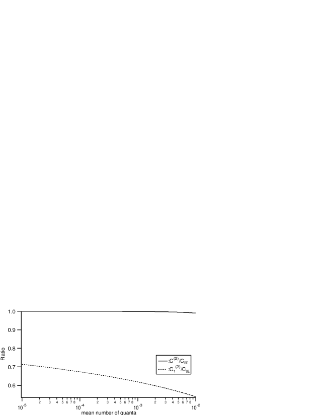
Figure 3: $C^{(2)}/C_{BE}$ and $C^{(2)}_{1}/C_{BE}$ with respect to mean number of quanta $m$

In Figure 3 the value of $C^{(2)}/C_{BE}$ is plotted with respect to the energy constraint $m$. The figure shows that the binary discretization realizes approximately the capacity $C_{BE}$ in a weak photon case ($m<10^{-2}$). Indeed, by applying $e^{-x}\approx 1-x$ and $\log(1-x)\approx-x$ to Eqs. (69) and (72) and neglecting the term of $m^{2}$, the following approximation holds,

$$C_{BE}\approx C^{(2)}\approx-m\log m+m\quad\quad\mbox{for }m\ll 1.$$ (73)

These results show that the coherent state channel can be simulated by the binary discrete channel in a weak photon case.

On the other hand, the classical continuous channel can not be simulated by any discrete channel[Cover:91]. In particular the binary discretization does not realize the capacity. To achieve the capacity, we must solve a more complicated optimization problem. The problem, related with the sphere packing, is still one of main topics in the classical information theory.

We shall consider another optimization, which is concerned with the maximum mutual information and formulated as follows,

$$C_{1}^{(2)}=\sup_{\{\alpha,\beta\}}\sup_{Q}\sup_{\{\hat{\Pi}_{\alpha},\hat{\Pi}_{\beta}\}}I_{d}(\{\alpha,\beta\},\{Q,1-Q\},\{\hat{\Pi}_{\alpha},\hat{\Pi}_{\beta}\}).$$ (74)

Here $I_{d}$ is the mutual information of the binary channel with input signals $\{|\alpha\rangle,|\beta\rangle\}$, the corresponding a priori probabilities $\{Q,1-Q\}$ and the signal detection process given by the positive operator-valued measure (POVM) $\{\hat{\Pi}_{\alpha},\hat{\Pi}_{\beta}\}$. The optimum POVM for two input letters consists of two detection operators [4], and hence we can restrict the number of the detection operators in Eq. (74) to two without loss of generality.

Let us solve the optimization problem. The right-hand side of Eq. (74) can be divided into two parts as follows,

$$C_{1}^{(2)}=\sup_{\{\alpha,\beta\}}\sup_{Q}I_{a}(\{\alpha,\beta\},Q)$$ (75)

$$I_{a}(\{\alpha,\beta\},Q)=\sup_{\{\hat{\Pi}_{1},\hat{\Pi}_{2}\}}I_{d}(\{\alpha,\beta\},\{Q,1-Q\},\{\hat{\Pi}_{1},\hat{\Pi}_{2}\}).$$ (76)

The accessible information is known [1] to be calculated as

$$I_{a}=I_{a}(\{\alpha,\beta\},Q)=H(Q)-H(f(\{\alpha,\beta\},Q)).$$ (77)

In this equation

$$H(Q)=-Q\log Q-(1-Q)\log(1-Q),$$ (78)

$$f=f(\{\alpha,\beta\},Q)=\frac{1}{2}\left(1-\sqrt{1-4\kappa^{2}Q(1-Q)}\right),$$ (79)

where

$$\kappa^{2}=|\langle\alpha|\beta\rangle|^{2}=\exp[-|\alpha-\beta|^{2}].$$ (80)

On the contrary to $C^{(2)}$, the quantity $C^{(2)}_{1}$ can be only obtained approximately: the optimum a priori distribution is given by

$$Q_{opt}(m)\approx\frac{-m\log m-m}{3},$$ (81)

and the optimum binary signals are $\{|\alpha{\rangle},|\beta{\rangle}\}$ satisfying $\beta=k\alpha$ $(-1\leq k\leq 0)$ and

$$|\alpha|^{2} = \frac{1-Q_{opt}(m)}{Q_{opt}(m)}m,$$ (82a)

$$|\beta|^{2} = \frac{Q_{opt}(m)}{1-Q_{opt}(m)}m.$$ (82b)

Then The value of $C_{1}^{(2)}$ is given by $I_{a}(Q_{opt}(m))$.

In Fig 3 the value of $C_{1}^{(2)}/C_{BE}$ is plotted with respect to the energy constraint $m$. The ratio $C_{1}^{(2)}/C_{BE}$ converges to 1 when $m\to 0$. This substantiates the validity of the Gordon’s suggestion in theory. However the convergence speed is very slow. For example $C_{1}^{(2)}/C_{BE}$ is 0.82 for $m=10^{-10}$, and then the capacity takes a very small value: $C_{BE}\approx 2.4\times 10^{-9}$. This shows the Gordon’s suggestion is not correct in practice. We can further obtain the following approximation of $C_{1}^{(2)}$, the value of which is larger than the capacity $\log(m+1)$ but is less than the capacities $C^{(2)}$, $C_{BE}$:

$$\begin{split}\log(m+1)&\leq C_{1}^{(2)}\approx-m\log m-m\\ &\leq C^{(2)}\approx C_{BE}\approx-m\log m+m\\ &\quad\quad\quad\mbox{ for }m\ll 1.\end{split}$$ (83)

Strictly speaking, $C_{1}^{(2)}$ should be compared to the maximum mutual information $C_{1}$ of the original quantum continuous channel. It is conjectured $C_{1}^{(2)}$ gives a good approximation of $C_{1}$, but we have no way of calculating $C_{1}$ for the quantum continuous channel.

7 Conclusion

In this review paper, applications of the general formulae for capacity in the quantum information theory to optical communication processes have been introduced. As a special result, we would like to emphasize that capacity formula was calculated for attenuated noisy channel by using Holevo’s general theory of capacity for continuous alphabet. This formula may provide the capacity formula in optical field which corresponds to Shannon capacity formula for Gaussian noise model in long distance microwave communication system.

References

- [1] M. Ban, K. Kurokawa, and O. Hirota. Cut-off rate performance of quantum communication channels with symmetric signal states. J. of Opt. B, Quantum Semiclass. Opt., 1:206–218, 1999.
- [2] M. Ban, K. Kurokawa, R. Momose, and O. Hirota. Optimum measurements for discrimination among symmetric quantum states and parameter estimation. Int. J. Theor. Phys, 36:1269–1288, 1997.
- [3] C. H. Bennett and P. W. Shor. Quantum information theory. IEEE Trans. on Information Theory, 44(6):2724–2742, 1998.
- [4] Davies. Information and quantum measurement. IEEE. Trans. Inform. Theory, 24:596–599, 1978.
- [5] C. A. Fuchs and C. M. Caves. Ensemble-dependent bounds for accessible information in quantum mechanics. Phys. Rev. Lett., 73:3047–3050, 1994.
- [6] C. A. Fuchs and A. Peres. Quantum state disturbance versus information gain: Uncertainty relations for quantum information. Phys. Rev. A, 53:2038–2045, 1996.
- [7] J. P. Gordon. Quantum effect in communications systems. IRE Proc., 50:1898–1908, 1962.
- [8] P. Hausladen, R. Joza, B. Schumacher, M. Westmoreland, and W. Wootters. Phys. Rev. A, 54:1869, 1996.
- [9] O. Hirota. A foundation of quantum channels with super additiveness for shannon information. Applicable Algebra in Eng. Communication and Computing, 10(4/5):401–427, 2000.
- [10] A. S. Holevo. Statistical detection theory for quantum systems. J. of Multivariable analysis, 3:337–394, 1973.
- [11] A. S. Holevo. The capacity of quantum communication channel with general signal states. IEEE Trans. Inform. Theory, 44:269–273, 1998.
- [12] A. S. Holevo. Coding theorems for quantum channels. Tamagawa University Research Review, 4(1), 1998.
- [13] A. S. Holevo, M. Sohma, and O. Hirota. Capacity of quantum gaussian channels. Phys. Rev. A, 59:1820–1828, 1999.
- [14] A. S. Holevo and R. F. Werner. Evaluating capacities of bosonic gaussian channels. Phys. Rev. A, 63:032312, 2001.
- [15] K. Kato, M. Osaki, and O.Hirota. Derivation of classical capacity of quantum channel for discrete information source. Physics Letters A, 251:157–163, 1999.
- [16] L. B. Levitin. Optimal quantum measurements for two pure and mixed states. Plenum Press, New York, ed by Belavkin, Hirota, and Hudson, 1995.
- [17] M. Osaki, M. Ban, and O. Hirota. J. of Modern Optics, 45:269–282, 1998.
- [18] M. Sasaki, K. Kato, M. Izutu, and O. Hirota. Quantum channels showing superadditivity in classical capacity. Phys. Rev. A, 58:146–158, 1998.
- [19] B. Schumacher and M. D. Westmoreland. Sending classical information via noisy quantum channel. Phys. Rev. A, 56(1):131–138, 1997.
- [20] K. Shimoda, H. Takahashi, and C.H.Townes. Fluctuations in amplification of quanta with application to maser amplifiers. J. Phys. Soc. Japan, 12(6):686, 1957.
- [21] M. Sohma and O. Hirota. Binary discretization for quantum continuous channels. Physical Review A, 62(5):052312–1–4, 2000.
- [22] H. P. Yuen and M. Ozawa. Ultimate information carrying limit of quantum systems. Phys. Rev. Lett., 70:363, 1993.