Opposite Arrows of Time Can Reconcile Relativity and Nonlocality

Abstract

We present a quantum model for the motion of $N$ point particles, implying nonlocal (i.e., superluminal) influences of external fields on the trajectories, that is nonetheless fully relativistic. In contrast to other models that have been proposed, this one involves no additional space-time structure as would be provided by a (possibly dynamical) foliation of space-time. This is achieved through the interplay of opposite microcausal and macrocausal (i.e., thermodynamic) arrows of time.
PACS numbers 03.65.Ud; 03.65.Ta; 03.30.+p

1 Introduction

We challenge in this paper a conclusion that is almost universally accepted: that quantum phenomena, relativity, and realism are incompatible. We show that, just as in the case of the no-hidden-variables theorems, this conclusion is hasty. And, as in the hidden variables case, we do so with a counterexample.

We present a relativistic toy model for nonlocal quantum phenomena that avoids the usual quantum subjectivity, or fundamental appeal to an observer, and describes instead, in a rather natural way, an objective motion of particles in Minkowski space. In contrast to that of [3], see below, our model invokes only the structure at hand: relativistic structure provided by the Lorentz metric and quantum structure provided by a wave function. It shares the conceptual framework—and forms a natural generalization—of Bohmian mechanics, a realistic quantum theory that accounts for all nonrelativistic quantum phenomena [4]. The key ingredient is a mechanism for a kind of mild backwards causation, allowing only a very special sort of advanced effects, that is provably paradox-free.

Unfortunately, the model considered here, unlike that of [3], does not provide any obvious, distinguished probability measure on the set of its possible particle paths, on which many of its detailed predictions are likely to be based. It is thus difficult to assess the extent to which the model is consistent with violations of Bell’s inequality [1]. However, in the nonrelativistic limit of small velocities (and slow changes in the wave function), the behavior of our model coincides with that of the usual Bohm–Dirac model [2] and is thus consistent with the $|\psi|^{2}$ distribution, and hence with violations of Bell’s inequality, in every frame in which the velocities are slow.

2 Spirit of the Model

The backwards causation arises from a time-asymmetric equation of motion for $N$ particles that involves advanced data about the other particles’ world lines. The asymmetry of this law defines an intrinsic arrow of time, which is not present in well-known theories like Newtonian mechanics or Wheeler–Feynman electrodynamics, and which we call the microcausal arrow of time, as opposed (and, indeed, opposite) to the usual, thermodynamic or macrocausal arrow of time.

In a recent paper [6], L. S. Schulman investigated the possibility of opposite thermodynamic arrows of time in different regions of the universe: that in some distant galaxy, entropy might decrease with (our) time, “eggs uncrack,” and inhabitants, if present, feel the arrow of time to be just opposite to what we feel. He studied this question in terms of statistical mechanics, and, on the ground of computer simulations, came to the conclusion that this is quite possible, apparent causal paradoxes notwithstanding. We also consider two opposite arrows of time, but not belonging to different regions of space-time, and not as a study in statistical mechanics, but as a possible explanation of quantum nonlocality. Instead of having the thermodynamic arrow of time vary within one universe, we consider the situation in which two conceptually different arrows of time, the microcausal and the macrocausal arrow, are everywhere opposite throughout the entire universe.

It has been suggested [3] that in order to account for quantum nonlocality, one employ—contrary to the spirit of relativity—a time-foliation, i.e., a foliation of space-time into 3-dimensional spacelike hypersurfaces, which serve to define a temporal order for spacelike separated points, or one might say simultaneity-at-a-distance, and hence simultaneity surfaces along which nonlocal effects propagate. This foliation is intended to be understood, not as a gauge (i.e., as one among many points of view a physicist may choose), but as an additional element of space-time structure existing objectively out there in the universe, defining in effect a notion of true simultaneity. In [3], the time-foliation is itself a dynamical variable subject to an evolution law. In contrast, the model we present here does not invoke a distinguished foliation.

In our model, the formula for the velocity of a particle at space-time point $p$ involves, in a Lorentz-invariant manner, the points where the world lines of the other particles intersect—not any “simultaneity surface” containing $p$ but rather—the future light cone of $p$, as well as the velocities of the particles at these points. As a consequence, it is easy to compute the past world lines from the future world lines, but it is not at all obvious how to compute the future from the past—except by testing all the uncountably many possibilities. One can say that the behavior of a particle at time $t$ has causes that lie in the future of $t$, so that on the microscopic level of individual particles and their world lines, the arrow of time of causation, as defined by the dynamics, points towards the past. We call this the microcausal arrow of time and denote it by $C$; it defines a notion of “$\mbox{future}_{C}$” = past, and of “$\mbox{past}_{C}$” = future. Thus the velocity of a particle depends on where the other particles intersect the $\mbox{past}_{C}$ light cone of that particle (effects are “retarded_C”). This microcausal arrow of time is also an arrow of determinism: knowledge of the world lines prior_C to a certain time determines the $\mbox{future}_{C}$, whereas there is no reason to believe the converse, that the $\mbox{future}_{C}$ determines the $\mbox{past}_{C}$.

Now consider the set of solutions of the law of motion as given, and consider those solutions which at a certain time $T$ in the distant $\mbox{future}_{C}$ reside in a certain macrostate with low entropy. We are interested in their behavior for times prior_C to $T$. One should expect that entropy decreases in the direction of $C$ until it reaches its minimum at $T$. So the thermodynamic arrow of time $\Theta$, as defined by the direction of entropy increase, is opposite to $C$ (see Fig. 1).

Figure 1: Boundary conditions are imposed on the $\mbox{future}_{C}=\mbox{past}_{\Theta}$ end of time. (The time direction is vertical.)

The arrow of time that inhabitants of this imaginary world would perceive as natural is the one corresponding to eggs cracking rather than uncracking, that is, the thermodynamic one. So when the inhabitants speak of the future, they mean $\mbox{future}_{\Theta}=\mbox{past}_{C}$. That is why we called $\mbox{past}_{C}$ the future in the beginning. It is $\Theta$ that corresponds to macroscopic causality.

The law of motion is Lorentz-invariant, and since it involves retarded_C but not advanced_C influences, it is local with respect to $C$, i.e. what is happening at a space-time point $p$ depends only on what happened within (and on) the $\mbox{past}_{C}$ light cone of $p$. With respect to $\Theta$, however, the law of motion is nonlocal, as the trajectory of a particle at $p$ depends on where and how the other particles cross the $\mbox{future}_{\Theta}$ light cone of $p$ (see Fig. 2), which again might be influenced by interventions of macroscopic experimenters at spacelike separation from $p$. So this law of motion provides an example of a theory that entails nonlocality (superluminal influences) while remaining fully Lorentz-invariant.

Figure 2: The 4-velocity of a particle at a space-time point $p$ depends on where the world lines of the other particles cross the $\mbox{past}_{C}$ light cone of $p$, and on the 4-velocities at these points.

It is important here to appreciate that the thermodynamic arrow of time arises not from any microscopic time asymmetry, but from boundary conditions of the universe. That is a moral of Boltzmann’s analysis of the emergence of the thermodynamic arrow of time from a time symmetric microscopic dynamics, where no microscopic time arrow is available as a basis of macroscopic asymmetry. As a consequence, the microscopic asymmetry present in our model should not affect the thermodynamic arrow $\Theta$ at all, and we should be free to choose the direction of $\Theta$ as either the same as or opposite to $C$, by imposing low-entropy boundary conditions at either the distant past_C or future_C when setting up the model. The advantage of having them opposite is that this allows our model to display nonlocal behavior. Had we chosen $\Theta$ to be in the same direction as $C$, then the model would have been local—because then what happens at $p$ would depend only on what had happened in the past light cone of $p$.

3 Equations of the Model

Now let us turn to the details of the model. It is similar to Bohmian mechanics [4], in the sense that velocities are determined by a wave function. In our case, the wave function is an $N$ particle Dirac spinor field, i.e., a mapping $\psi:(\mbox{space-time})^{N}\to(\mathbb{C}^{4})^{\otimes N}$. We consider entanglement, but without interaction. The wave function is supposed to be a solution of the multi-time Dirac equation

$$\mathbf{1}\otimes\cdots\otimes\underbrace{\gamma^{\mu}}_{i\mathrm{th\>\>place}}\otimes\cdots\otimes\mathbf{1}\>(i\hbar\partial_{i,\mu}+eA_{\mu}(x_{i}))\>\psi=m\psi$$

where summation is understood for $\mu$ but not for $i$, $m$ is the mass parameter, $e$ the charge parameter, $\gamma^{\mu}$ are the Dirac matrices, $A_{\mu}$ is an arbitrary given 1-form (the external electromagnetic vector potential), and $i$ runs from 1 through $N$ enumerating the particles.

For any space-time point $p$ and any parametrized timelike curve $x^{\mu}(s)$, let $s_{\mathrm{ret}}(p)$ denote the value of $s$ such that $x^{\mu}(s)$ lies on the $\mbox{past}_{C}$ light cone of $p$. Our law of motion demands of the world lines $x^{\mu}_{i}(s_{i})$ of the $N$ particles that (a) they be timelike and (b) for every particle $i$ and parameter value $s_{i}$,

$$\frac{dx^{\mu_{i}}_{i}}{ds_{i}}\>\bigg{\|}\>\overline{\psi}\,(\gamma^{\mu_{1}}\otimes\cdots\otimes\gamma^{\mu_{N}})\,\psi\prod_{j\neq i}\frac{dx^{\nu_{j}}_{j}}{ds_{j}}\big{(}s_{\mathrm{ret},j}(p_{i})\big{)}\eta_{\mu_{j}\nu_{j}}\,,$$ (1)

where $\|$ means “is parallel to” (i.e. is a multiple of), $p_{i}=x_{i}(s_{i})$, $s_{\mathrm{ret},j}$ refers to the $x_{j}$ world line, $\overline{\psi}=\psi^{\dagger}\gamma^{0}\otimes\cdots\otimes\gamma^{0}$, $\eta=\mbox{diag}(1,-1,-1,-1)$ is the Minkowski metric, and $\psi$ and $\overline{\psi}$ are evaluated at $\left(x_{1}\left(s_{\mathrm{ret},1}(p_{i})\right),\ldots,x_{N}\left(s_{\mathrm{ret},N}(p_{i})\right)\right)$.

Here is what the law says. Suppose that space-time point $p_{i}$ is on the world line of particle $i$. Then the velocity of particle $i$ at $p_{i}$ is given as follows: Find the points of intersection $p_{j}$ of the world lines of the other particles with the $\mbox{past}_{C}$ light cone of $p_{i}$, and let $u^{\nu}_{j}=dx^{\nu}_{j}/ds_{j}$ be the 4-velocities at these points. (It does not matter whether or not $u$ is normalized, $u^{\nu}u_{\nu}=1$.) Evaluate the wave function at $(p_{1},\ldots,p_{N})$ to obtain an element $\psi$ of $(\mathbb{C}^{4})^{\otimes N}$, and compute also $\overline{\psi}$. Use these to form the tensor $J^{\mu_{1}\ldots\mu_{N}}=\overline{\psi}\gamma^{\mu_{1}}\otimes\cdots\otimes\gamma^{\mu_{N}}\psi$. $J$ is an element of $T_{p_{1}}M\otimes\cdots\otimes T_{p_{N}}M$, where $M$ stands for the space-time manifold and $T_{p}$ denotes the tangent space at the point $p$. Now for all $j\neq i$, transvect $J$ with $u^{\nu_{j}}_{j}\eta_{\mu_{j}\nu_{j}}$. This yields an element $j_{i}^{\mu_{i}}$ of $T_{p_{i}}M$, defining a 1-dimensional subspace $\mathbb{R}j_{i}^{\mu_{i}}$ of $T_{p_{i}}M$. The world line of particle $i$ must be tangent to that subspace. (One easily checks that this prescription is purely geometrical: it provides a condition on the collection of space-time paths that does not depend on how they are parametrized. The velocity is not defined if $\psi(p_{1},\ldots,p_{N})=0$—and only in that case, as we will see below.)

How does one arrive at this law? To begin with, there is an obvious extension of Bohmian mechanics to a single Dirac particle [2]. Let $\psi:(\mbox{space-time})\to\mathbb{C}^{4}$ obey the Dirac equation, let $j^{\mu}=\overline{\psi}\,\gamma^{\mu}\,\psi$ be the usual Dirac probability current, and let the integral curves of the 4-vector field $j^{\mu}$ be the possible world lines of the particle, one of which is chosen at random. The world lines are timelike, and therefore intersect every spacelike hyperplane precisely once. If this point of intersection is $|\psi|^{2}$ distributed in one frame at one time, it is $|\psi|^{2}$ distributed in every frame at every time. That is because the Dirac equation implies that $j^{\mu}$ is a conserved current, $\partial_{\mu}j^{\mu}=0$, and because in every frame $|\psi|^{2}=j^{0}$. For $N=1$, our law of motion reproduces this single-particle law.

This Bohm–Dirac law of motion possesses an immediate many-particle analogue if one is willing to dispense with covariance [2]: using the simplest tensor quadratic in $\psi$, $J^{\mu_{1}\ldots\mu_{N}}=\overline{\psi}\,\gamma^{\mu_{1}}\otimes\cdots\otimes\gamma^{\mu_{N}}\,\psi$, one can write

$$\frac{dx^{\mu_{i}}_{i}(s)}{ds}\>\bigg{\|}\>J^{0\ldots\mu_{i}\ldots 0}(p_{1},\ldots,p_{N})$$ (2)

for the velocities, where $p_{1},\ldots,p_{N}$ are simultaneous (with respect to one preferred Lorentz frame) and $s$ is again an arbitrary curve parameter. This motion also conserves the probability density $\rho=|\psi|^{2}=J^{0\ldots 0}$. It can be generalized [3] to arbitrary spacelike hypersurfaces (rather than the parallel hyperplanes corresponding to a Lorentz frame). The hypersurfaces then play a twofold role: first, the multi-time field $J$ is evaluated at $N$ space-time points $p_{1},\ldots,p_{N}$ which are taken to lie on the same hypersurface. Second, the unit normal vectors on the hypersurface are used for contracting all but one of the indices of $J^{\mu_{1}\ldots\mu_{N}}$ to arrive at a 4-vector [3]; that is how the 0-components arise in (2). So (1) is merely a modification of known “Bohmian” equations, using a simple strategy for avoiding the use of distinguished spacelike hypersurfaces: use light cones as the hypersurfaces for determining the $N$ space-time points, and use the velocity 4-vectors (of the other particles) for contracting all but one of the indices of $J$. (If vectors normal to the light cone had been used, the model would not have a good nonrelativistic limit; see below.)

“Bohmian” equations of motion usually imply that positions can be taken to always be $|\psi|^{2}$ distributed. That is what makes Bohmian mechanics compatible with the empirical facts of quantum mechanics. In contrast, our velocity formula (1) does not conserve the $|\psi|^{2}$ distribution, and that is why we call it a toy model rather than a serious theory. In the nonrelativistic limit, however, our model coincides with the many-particle Bohm–Dirac law, since the future light cone approaches the $t=\mathrm{const}$ hyperplane, and hence is compatible with a $|\psi|^{2}$ distribution, consistent with quantum mechanics. Note also that, due to Bell’s theorem [1], a necessary condition for compatibility of a law of motion with the $|\psi|^{2}$ distribution is its nonlocality. So a necessary step towards such a law that is relativistic is to come up with a covariant method of providing nonlocality: we develop one such method here.

The question remains as to whether for $\psi\neq 0$, $j_{i}^{\mu}$ is timelike. Actually, it is sometimes lightlike: e.g., for $\psi(p_{1},\ldots,p_{N})=\frac{1}{2}(1,1,1,-1)\otimes\psi^{\prime}$ in the standard representation with $\psi^{\prime}\in(\mathbb{C}^{4})^{\otimes(N-1)}$, one finds that $j_{1}^{\mu}=(1,0,0,1)$. But this is an exceptional case like $\psi=0$. To see that $j_{i}^{\mu}$ is either timelike or lightlike, note that a vector is nonzero-timelike-or-lightlike if and only if its scalar product with every timelike vector is nonzero. So pick a nonzero timelike vector, call it $u_{i}^{\nu_{i}}$, and compute the scalar product

$$\lambda:=j_{i}^{\mu_{i}}u_{i}^{\nu_{i}}\eta_{\mu_{i}\nu_{i}}=\overline{\psi}\,(\gamma^{\mu_{1}}\otimes\cdots\otimes\gamma^{\mu_{N}})\,\psi\>\prod_{j}u_{j}^{\nu_{j}}\eta_{\mu_{j}\nu_{j}}\,.$$

Without changing the absolute value of $\lambda$, we can make sure all $u_{j}$s are future-pointing (i.e. $u_{j}^{0}>0$), replacing $u_{j}$ by $-u_{j}$ if necessary. Through a suitable choice of $N$ Lorentz transformations in the spaces $T_{p_{1}}M,\ldots,T_{p_{N}}M$, we can replace all $u_{j}$s by $(1,0,0,0)$ while also replacing $\psi$ by a transformed spinor $\psi^{\prime}$. Thus $\pm\lambda=\overline{\psi^{\prime}}\,(\gamma^{0}\otimes\cdots\otimes\gamma^{0})\,\psi^{\prime}=(\psi^{\prime})^{\dagger}\psi^{\prime}>0$ unless $\psi^{\prime}=0$, i.e., unless $\psi=0$.

4 Properties of the Model

The model is of course very restricted in the sense that we do not allow for interaction between the particles. While it is difficult to find global solutions to this law of motion, it is quite obvious how to obtain a solution from initial_C (=final_Θ) boundary counditions: for computing the velocities of all particles at any time $t=t_{0}$, data are needed about velocities of the particles at several earlier_C (=later_Θ) instants of time (see Fig. 3), and all such data are available given the world lines prior_C to (=after_Θ) $t_{0}$. While propagation in our model from microcausal past to microcausal future is far from routine, it is thus ordinary enough to make it seem reasonable that there should exist a unique continuation of a given past_C to the future_C that obeys the law in that future, even if the specified past_C does not. This of course does not prove, even heuristically, the existence of global solutions, existing for all times, past, present, and future, but for our purposes this does not matter so much. For our purposes, i.e., for arguing for the existence of relevant solutions, it is sufficient to consider the specification of the past_C up to a certain time in the spirit of an initial (or final) boundary condition, from which evolution takes place.

Figure 3: For computing velocities at $t=t_{0}$, information about several space-time points, lying at different times, is relevant: where the crossing points (dots) through the light cones are, and what the velocities are at these points.

We note that our approach has little if any overlap with the proposals of Huw Price [5], who argues that backwards causation can “solve the puzzles of quantum mechanics.” Whereas Price seeks to exploit backwards causation to avoid nonlocality, we use it to achieve nonlocality in a Lorentz invariant way. Moreover, while our model involves advanced effects on particle trajectories, we do not propose any advanced effects on the wave function, as does Price [5, p.132].

We have reason to believe that in our model, (macro) causes precede (macro) effects. To be sure, why causality proceeds in one direction alone is not easy to understand, even without a micro arrow. The usual understanding grounds this in low entropy “initial” conditions, and the same considerations should apply even when there is a micro arrow, even when this arrow points (in a reasonable sense) in the opposite direction. Consequently, macrocausality, which is what usual causal reasoning involves, should follow the thermodynamic arrow of time.

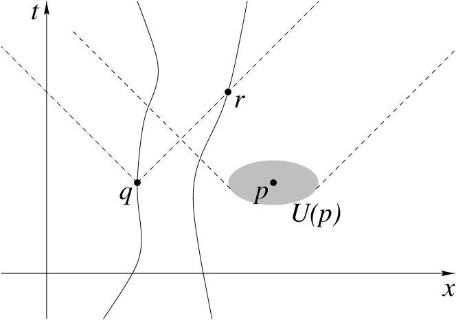
Figure 4: Changing the external potential in the space-time region $U(p)$ affects the wave function only in the absolute future_Θ of $U(p)$. But this means that $\psi(q,r)$ is changed, so that the velocity at $q$ is likely to be affected.

To see how this interplay between micro- and macro-causality plays out in our model, consider two electromagnetic potentials $A_{\mu}$ and $A_{\mu}^{\prime}$ that differ only in a small space-time region $U(p)$ around the point $p$ (see Fig. 4). Solving the multi-time Dirac equation for the same initial_Θ wave function gives two functions $\psi,\psi^{\prime}$ which differ only for those $N$-tuples $(p_{1},\ldots,p_{N})$ of space-time points for which at least one $p_{i}$ lies inside or on the $\mbox{future}_{\Theta}$ light cone of some $\widetilde{p}\in U(p)$. We can regard effects on the wave function as always after_Θ the external cause. Not so for the world lines; in general, effects of $A_{\mu}^{\prime}(p)$ will be found everywhere: in the future, past and present of $p$. More precisely, given a solution $S$ (an $N$-tuple of paths) of the law of motion for $\psi$, there will be no corresponding solution $S^{\prime}$ of the law of motion for $\psi^{\prime}$ such that $S$ and $S^{\prime}$ agree in the past of $U(p)$, or in the future of $U(p)$. So on the particle level, causation is effectively in both time directions. Note that this cannot possibly lead to causal paradoxes since there is no room for paradoxes in the Dirac equation and our law of motion.

This is essentially because there is no feedback mechanism which could lead to causal loops. Instead, the Dirac equation may be solved in the ordinary way from past to future, starting out from an initial_Θ wave function, and the equation of motion can subsequently be solved from initial_C conditions. Thus, insofar as the microscopic dynamics is concerned, there is no way a paradox could possibly arise. This proves consistency even for a universe governed as a whole by our law of motion. In this respect, the situation is much different with Wheeler–Feynman electrodynamics, tachyons, and theories involving closed timelike curves, since they all have microcausal feedback, so that even the existence of solutions is dubious for given initial data.

One last remark concerning the question, touched upon earlier, of whether macroscopic backwards causation is possible in our model (i.e., whether observable events in the future can cause observable effects in the past): the nonlocal backwards microcausal mechanism in our model is based on quantum entanglement, which is now widely regarded as giving rise to a rather fragile sort of nonlocality, revealed through violations of Bell’s inequality, that does not support the sort of causal relationship between observable events that can be used for signalling. (For our model, however, things are trickier than usual since no-signalling results are grounded on the $|\psi|^{2}$ distribution.)

In the nonrelativistic limit $c\to\infty$, the unusual causal mechanism of our model is replaced by a more conventional one: as mentioned earlier, the future light cone (and the past light cone, as well) approaches the $t=t_{0}$ hypersurface, so instead of having to find the points where the other world lines cross the future light cone, one needs to know the points where the other world lines cross the $t=t_{0}$ hypersurface (which in the nonrelativistic limit does not depend on the choice of reference frame). This means that the configuration of the particle system at time $t_{0}$ determines directly all the velocities and thus the evolution of the configuration into the future (or the past, as well). Thus the nonrelativistic limit of our model is causally routine, and our model can be regarded as illustrating how a simple small deviation from this normal picture, imperceptible in the nonrelativistic domain, can provide a relativistic account of nonlocality. In fact, it is easy to see that in the nonrelativistic limit of small velocities and slow changes in the wave function, our model coincides with the usual Bohm–Dirac model [2], so that it is then compatible with a $|\psi|^{2}$ distribution of positions and thus with the Bell–EPRB correlations.

5 Conclusions

We have proposed that in our relativistic universe quantum nonlocality originates in a microcausal arrow of time opposite to the thermodynamic one. We recognize that this proposal is rather speculative. However, we believe it is a possibility worth considering.

Acknowledgements. We are grateful for the hospitality of the Institut des Hautes Études Scientifiques (I.H.E.S.), Bures-sur-Yvette, France, where the idea for this paper was conceived. The paper has profited from questions raised by the referees.

References

- [1] J.S. Bell: Speakable and unspeakable in quantum mechanics (Cambridge University Press, 1987).
- [2] D. Bohm and B.J. Hiley: The Undivided Universe: An Ontological Interpretation of Quantum Theory (Routledge, Chapman and Hall, London, 1993) page 274.
- [3] D. Dürr, S. Goldstein, K. Münch-Berndl, and N. Zanghì: Phys. Rev. A 60, 2729 (1999) arXiv: quant-ph/9801070.
- [4] D. Dürr, S. Goldstein, and N. Zanghì: “Bohmian Mechanics as the Foundation of Quantum Mechanics,” in Bohmian Mechanics and Quantum Theory: An Appraisal, ed. by J.T. Cushing, A. Fine, S. Goldstein (Kluwer Academic, Dordrecht, 1996) arXiv: quant-ph/9511016.
- [5] H. Price: Time’s Arrow and Archimedes’ Point (Oxford University Press, 1996).
- [6] L.S. Schulman: Phys. Rev. Lett. 83, 5419 (1999) arXiv: cond-mat/9911101.