Abstract

We present a theoretical analysis of inequivalent classes of interference experiments with non-abelian anyons using an idealized Mach-Zender type interferometer. Because of the non-abelian nature of the braid group action one has to distinguish the different possibilities in which the experiment can be repeated, which lead to different interference patterns. We show that each setup will, after repeated measurement, lead to a situation where the two-particle (or multi-particle) state gets locked into an eigenstate of some well defined operator. Also the probability to end up in such an eigenstate is calculated. Some representative examples are worked out in detail.

I Introduction

Physics in lower dimensions is not always simpler. A nontrivial instance in two dimensions is the possibility of anyons, i.e. excitations which exhibit statistics properties which transcend the conventional possibilities of bosons and fermions [1]. It is striking that such exotic theoretical possibilities appear to be realized in nature. With the experimental advances in condensed matter physics related to the fractional Quantum Hall effect, quasi-particles have been discovered that appear to exhibit anyonic behavior.

There is also a more mundane interest in the two dimensional physics of anyons in the emerging field of quantum computation. In quantum computation, as the number of qubits grows, the problem of beating decoherence becomes a major threat: the larger the quantum system to be manipulated gets, the more it interacts with the (noisy) environment, causing the quantum state to collapse. In order to compensate the inaccuracies caused by decoherence, the idea of fault-tolerance and error-correction has become an important subject, and quantum codes were devised where single qubit-information is encoded into multiple qubits [2]. If errors in the physical qubits can be corrected in time, the stored quantum information remains intact, or at least the decoherence time of the encoded qubit is increased. The progress achieved in the theory of quantum error codes however is mainly mathematical in nature. Current experimental realizations of this idea of qubit-encoding do not yet share the optimism of the theorists and are still far from being decoherence free.

It may therefore be profitable to go back to some basic physics and search for intrinsically decoherence free quantum states. Promising candidates are “global quantum states” carrying quantum information that is not ‘stored’ locally, in single spins for instance, but in a robust collective property of a multi-particle system – a topological feature for example. Such a global characteristic of the state cannot be destroyed by local interactions, especially not by those with the noisy environment. As anyons exhibit such a global, topological robustness as a basic property, it seems anyons are especially suited for this kind of the quantum computer game, which goes by names as topological quantum computation [3] and geometrical quantum computation [4].

Anyons for quantum computation can be divided in two groups: the (conventional) abelian anyons which are manipulated by mere geometric (abelian) phases, as in [4, 5], and, most promising, the so-called non-abelian anyons (which are strictly speaking a generalization of the abelian anyons). Non-abelian anyons may carry non-trivial internal degrees of freedom which can have non-abelian topological interactions which allow (in principle) for a rather clean manipulation of entangled states. These non-abelian anyons may serve as intrinsically fault-tolerant decoherence free qubits[3, 6, 7, 8]. One might think of non-abelian anyons in particular media with for example broken symmetries which support quasi-particle excitations with anyonic properties as in model systems like the so-called discrete gauge theories [9, 10, 11].

A sometimes underestimated issue but necessary requirement for quantum computation is the ability to perform a measurement of the quantum state. In [6, 7, 8], the so-called fusion properties of the non-abelian anyons are used to perform a quantum measurement. But a perhaps more general applicable way to approach measurements, is to look at interference experiments with the quasi-particles, both for non-abelian anyons, as suggested by [3], and abelian anyons, [12]. Interference experiments with non-abelian anyons are generalizations of the Aharonov-Bohm effect, and have been studied in the past [13, 14]; however, these papers focussed primarily on determining the cross-section via the initial probability distribution, and neglected the change in the quantum state of the target particle. For topological quantum computation, the quantum state of the target particle, i.e., the qubit one likes to measure, obviously is important.

Motivated by these considerations, we have analyzed certain types of idealized interference experiments which one could perform with non-abelian anyons, thereby taking into account the changes in the quantum states of the quasi-particles. This leads to a critical study of the non-abelian generalization of the Aharonov-Bohm effect and how it could be measured by a Mach-Zender type device . It turns out that there are essentially different possibilities to perform the repeated experiment leading to very different interference patterns.

The paper is organized as follows, after a brief introduction to non-abelian anyons and the braid group we discuss in section II the general setup of experiments with the Mach-Zender interferometer. In section III we use this setup to analyze the different classes of anyonic experiments that could be performed and show to what kinds of interference patterns they may lead. We distinguish the so-called one-to-one, many-to-one and many-to-many experiments. The observable patterns may be very distinct, because after a sufficient number of repetitions the system will get locked into a particular eigenstate or subspace of some well determined operator which depends on the type of experiment. The proof of this locking is relegated to the appendix. The probabilities of finding certain patterns is also calculated. At the end of the paper we have summarized the results for the various classes in a comprehensive way in Table IV.

A Non-abelian anyons and the braid group

If we physically move two particles around each other and return both to their original position, this corresponds to a closed path in the two-particle configuration space. In three or more dimensions this closed loop will be contractible to a point, which means that the monodromy operator describing the net effect on the two-particle Hilbert-space will just be the identity operator. If we take two identical (indistinguishable) particles one may also consider the exchange operator defined as the square root of the monodromy operator, which consequently can only have two distinct eigenvalues namely plus or minus one corresponding to bosons and fermions respectively. It is well known that in two dimensions the situation is fundamentally different; the loop is no longer contractible so that the (unitary) monodromy operator can generate an arbitrary phase. Similarly the exchange operator $R$ may yield any phase on a state with two identical particles which are therefore denoted as anyons. For such particles the anti-clockwise exchange operator ${\cal R}$ and the clockwise exchange ${\cal R}^{-1}$ have to be distinguished.

On an algebraic level this leads to a considerable generalization because it allows also the possibility of nontrivial braidings between different types of particles. In short, the simple representation theory of the symmetric group $S_{n}$ (of permutations) has to be replaced by the representation theory of the braid group $B_{n}$ which is in principle an infinite group. The one dimensional unitary representations of $B_{n}$ are labeled by an arbitrary phase, but its higher dimensional unitary irreducible representations are far more complicated. In general the n-particle Hilbert space can be decomposed in subspaces that will carry irreducible representations of this braid group $B_{n}$ and if such representations turn out to be higher dimensional we call the particles involved, non-abelian anyons.

The braid group $B_{n}$ is generated by $n-1$ elements $\tau_{i}$ and their inverses. The $\tau_{i}$ obey the Yang–Baxter equations, also known as the braid relations, which are:

$$\tau_{i}\tau_{i+1}\tau_{i}=\tau_{i+1}\tau_{i}\tau_{i+1}\quad\quad i=1,\ldots,n-2$$ (1)

$$\tau_{i}\tau_{j}=\tau_{j}\tau_{i}\quad\quad|i-j|\geq 2$$ (2)

The correspondence between the Yang–Baxter equations and braids of strings of rope is best described pictorially, as in Fig. 1.

FIG. 1.: A pictorial representation of the Yang-Baxter equations $\tau_{i}\tau_{i+1}\tau_{i}=\tau_{i+1}\tau_{i}\tau_{i+1}$ and $\tau_{i}\tau_{j}=\tau_{j}\tau_{i}$ with $|i-j|\geq 2$ for $i=1$ and $j=3$; the similarity with braids of strings of ropes is crystal-clear.

The way in which non-abelian anyons are usually described, is by endowing the particles with some internal degrees of freedom, the non trivial braid statistics of these particles can than be implemented by coupling these new internal degrees of freedom to a non-abelian Chern-Simons (or statistical) gauge field which mediates the appropriate type of topological interactions.

As different braidings need not commute, it becomes important to be able to distinguish between them. A convenient way to accomplish this is to order the system in the following way: map all particles in the two-dimensional plane on some fixed line and number the particles (we will take the line to be horizontal and we number r from right to left, starting with one). If particles $i$ and $i+1$ pass each other on the virtual line, we have to apply the appropriate exchange operator: ${\cal R}_{i}$ if the exchange is anti-clockwise, ${\cal R}^{-1}_{i}$ if clockwise (not that after the exchange the original particle $i$ now is particle $i+1$ and vice versa). Every braid can be decomposed as a product of these braids of adjacent particles, ${\cal R}_{i}$ and ${\cal R}^{-1}_{i}$; also known as the braid operators, ${\cal R}_{i}$ and ${\cal R}^{-1}_{i}$ clearly satisfy the braid relations (1), (2). An example is shown in Fig. 2.

FIG. 2.: An example on ordering a system with anyons and classifying braids. We assign a number to all six particles and map them on a (horizontal) line. The shown braid, which moves particle 3 around some of the other particles and back to its original position, can now be unambiguously decomposed in adjacent particle exchanges; read from right to left this particular braid is given by: ${\cal R}_{2}^{-2}{\cal R}_{3}{\cal R}_{4}{\cal R}_{5}^{2}{\cal R}_{4}^{-1}{\cal R}_{3}$.

Associated with each particle is an internal space, and identical particles carry identical internal spaces. Typically, and this probably is the main feature of non-abelian anyons, the internal states of different particles may become entangled through braiding: this interaction of the non-abelian anyons is of a topological nature, independent of the distance between the anyons, and it is a global property of the system, unperturbable by local interactions. The total system’s, multi-particle, possibly entangled, internal state denoted by $|\psi\rangle$ lies in the tensor product of the internal spaces of the individual particles. In such tensor products we use the same ordering of particles as introduced above, in that particles which are left (right) on the virtual line should appear left (right) in the tensor product. For instance, imagine a system with one particle of type $A$ (with internal space $V^{A}$) and two particles of type $B$ (with internal spaces $V^{B}$) which lie left of particle $A$. The three-particle internal state $|\psi\rangle$ is then an element of $V^{B}\otimes V^{B}\otimes V^{A}$.

The exchange caused by braid operators is made explicitly in the tensor product as well, i.e.: ${\cal R},{\cal R}^{-1}:V^{B}\otimes V^{A}\to V^{A}\otimes V^{B}$. We can think of ${\cal R}$ and ${\cal R}^{-1}$ as combination of some matrix and an operator $\sigma$, where $\sigma$ only swaps the two vector spaces. The matrix components of ${\cal R}$ and ${\cal R}^{-1}$ depend only on the types of the two particles that is operated upon. The square of ${\cal R}$, the monodromy operator ${\cal R}^{2}$, obviously does no net swapping and can be regarded as a unitary matrix, of which the explicit matrix-components depend on the particles on which it operates.

For the work we are about to present the knowledge of the braidmatrices is assumed a priori. It is clearly of great importance to understand the way one gets to this knowledge from an underlying algebraic structure. For two-dimensional physics there turns out to be an important generalization of ordinary group theory – the theory of quantum groups and Hopf algebra’s – which provides the natural descriptions of non-abelian anyons, in that it generates natural representations of the braid operator $R$ on the tensor product of its representations. For the Fractional Quantum Hall Effect for example, this programme has been carried out quite explicitly [15, 16]. This has evolved into a rapidly expanding field of research on its own, we will however not make explicit use of this machinery in the following.

II The setup of experiments with the Mach-Zender interferometer

We introduce the setup of our thought experiments using the Mach-Zender interferometer in this section. We will first treat an ordinary interference experiment, then move to the Aharonov-Bohm experiment, and generalize it further to the non-abelian anyon experiment. We will see that for non-abelian anyons, there is a nontrivial difference between the interference pattern and the probability distribution.

A Ordinary interference

We are interested in describing interference experiments with non-abelian anyons, which basically means that we investigate non-abelian generalizations of the Aharonov-Bohm effect. We should realize that it is not the topological interactions leading to the well known (phase) factors that cause the interference, for these interactions will only be able to modify existing interference patterns. So, the starting point is a basic device that produces ordinary interference effects, as such a device, we may for example choose the Mach-Zender interferometer. We will introduce some terminology that we like to use in the following sections without further reference.

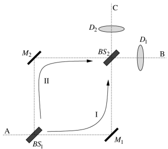
FIG. 3.: The setup of the Mach-Zender interferometer for ordinary interference experiments. At point A a particle may be injected in the device, where it will encounter beam splitter $BS_{1}$. It may traverse two different paths (thereby passing either mirror $M_{1}$ or $M_{2}$): the counterclockwise path I and pick up the phase factor $e^{i\theta_{\text{I}}}$, or the clockwise path II and acquire $e^{i\theta_{\text{II}}}$. The particle is not restricted to one path exclusively: it is allowed to travel both paths at the same time. Beam splitter $BS_{2}$ unites both paths, which now interfere with each other, and the particle emerges at one of two possible exits, B or C, which will be observed by a detector, $D_{1}$ or $D_{2}$.

The Mach-Zender interferometer, as depicted in Fig. 3, is a two dimensional device, built of two lossless beam splitters $BS_{1}$ and $BS_{2}$, two 100% reflecting mirrors $M_{1}$ and $M_{2}$, and two detectors $D_{1}$ and $D_{2}$. A particle enters the apparatus at point A on the left, where it encounters a beam splitter $BS_{1}$. The beam splitter will direct the particle along the counterclockwise path I and/or the clockwise path II. Both paths include a 100% reflecting mirror, $M_{1}$ or $M_{2}$, and both paths end up at beam splitter $BS_{2}$. The particle may now emerge from the apparatus at either point $B$ and be registered by detector $D_{1}$ or at point $C$ and be observed by detector $D_{2}$.

Ordinary interference is caused by the difference in relative phase of particles traveling along path I or path II, which is due to a difference in path length. We assume that we can adjust the apparatus in such a way that we can tune the difference in path length between paths I and II with high precision. We also have to include the transmission and reflection coefficients $t_{i},r_{i},t^{\prime}_{i},r^{\prime}_{i}$ of the beam splitters $BS_{i}$, see Fig. 4, because these complex factors also affect the relative phase. Since we assume the beam splitters to be perfect, its coefficients form a unitary matrix and we have that [17, 18]:

$$r_{i}^{*}=r_{i}^{\prime},\quad\quad t_{i}^{*}=-t^{\prime}_{i},\quad\quad|r_{i}|+|t_{i}|^{2}=1.$$ (3)

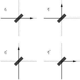
FIG. 4.: The coefficients $t_{i}$, $r_{i}$, $t^{\prime}_{i}$, $r^{\prime}_{i}$ determine the lossless beam splitter $BS_{i}$ (where $i=1,2$); $t_{i}$ indicates transmission for incoming beams from the left, $r_{i}$ stands for reflection when incident from the left, $t^{\prime}_{i}$ and $r^{\prime}_{i}$ denote transmission and reflection when incident from below.

We will not explicitly need the lengths of paths I and II, only the relative phases that the particle will acquire when traversing path I or II. We will indicate the associated phase factors by $e^{i\theta_{\text{I}}}$ and $e^{i\theta_{\text{II}}}$. The amplitude $A[D_{1}]$ of the particle’s wave packet component at detector $D_{1}$ is the sum of the contributions of both paths with the appropriate factors:

$$A[D_{1}]=t_{1}r^{\prime}_{2}e^{i\theta_{\text{I}}}+r_{1}t_{2}e^{i\theta_{\text{II}}},$$ (4)

and for $A[D_{2}]$:

$$A[D_{2}]=t_{1}t^{\prime}_{2}e^{i\theta_{\text{I}}}+r_{1}r_{2}e^{i\theta_{\text{II}}}.$$ (5)

The probabilities $P[D_{1}]$ and $P[D_{2}]$ that indicate the probability for the particle to be detected at $D_{1}$ or $D_{2}$ are the absolute squares of the amplitudes $A[D_{1}]$ and $A[D_{2}]$:

$$P[D_{1}]=|t_{1}r^{\prime}_{2}|^{2}+|r_{1}t_{2}|^{2}+2\,\text{Re}\!\left(t_{1}r^{\prime}_{2}r^{*}_{1}t^{*}_{2}e^{i(\theta_{\text{I}}-\theta_{\text{II}})}\right),$$ (6)

$$P[D_{2}] = |t_{1}t^{\prime}_{2}|^{2}+|r_{1}r_{2}|^{2}+2\,\text{Re}\!\left(t_{1}t^{\prime}_{2}r^{*}_{1}r^{*}_{2}e^{i(\theta_{\text{I}}-\theta_{\text{II}})}\right)$$ (7)

$$= |t_{1}t^{\prime}_{2}|^{2}+|r_{1}r_{2}|^{2}-2\,\text{Re}\!\left(t_{1}t^{*}_{2}r^{*}_{1}r^{\prime}_{2}e^{i(\theta_{\text{I}}-\theta_{\text{II}})}\right),$$ (8)

where we used (3) to go from (7) to (8). Adding eqs. (6) and (8) confirms that the total probability is of course preserved:

$$P[D_{1}]+P[D_{2}]=1.$$ (9)

In a real experimental setup, the particles that are directed at the apparatus will not all acquire precisely the same phase factors $e^{i\theta_{\text{I}}}$ or $e^{i\theta_{\text{II}}}$, for instance because of a slight difference in the momenta of the incoming particles. Therefore, we introduce a variable $q$ and a density function $\rho(q)$ to incorporate all such factors that influence the relative phase factors (which are due to the experimental setup). When calculating probabilities, we have to integrate over the, now $q$ dependent, phase factors $e^{i\theta_{\text{I}}(q)}$, $e^{i\theta_{\text{II}}(q)}$:

$$\int e^{i[\theta_{\text{I}}(q)-\theta_{\text{II}}(q)]}\rho(q)dq\equiv Qe^{i\theta},$$ (10)

where $Q$ is real and between zero and one, and $\theta$ is some sort of average phase difference. After integration over $q$, the probabilities of eqs. (6) and (8) then become:

$$P[D_{1}]=|t_{1}r^{\prime}_{2}|^{2}+|r_{1}t_{2}|^{2}+2Q\,\text{Re}\!\left(t_{1}r^{\prime}_{2}r^{*}_{1}t^{*}_{2}e^{i\theta}\right),$$ (11)

$$P[D_{2}]=|t_{1}t^{\prime}_{2}|^{2}+|r_{1}r_{2}|^{2}-2Q\,\text{Re}\!\left(t_{1}r^{\prime}_{2}r^{*}_{1}t^{*}_{2}e^{i\theta}\right).$$ (12)

We will use $e^{i\theta_{\text{I}}}$ and $e^{i\theta_{\text{II}}}$ in our notation for amplitudes, and $Q$ and $e^{i\theta}$ for probabilities, without further mentioning the implied $q$-integration.

So far, we have only talked about probabilities for single particles to be injected and observed. Obviously, we want to repeat many of such single particle ‘runs’ and call the result the interference pattern. In other words, the interference pattern $I[D_{1}]$ is the number of times $\#[D_{1}]$ that a particle is injected in the apparatus and observed by detector $D_{1}$ divided by the total number $n$ of injected particles, and likewise for $I[D_{2}]$:

$$I[D_{1}]=\frac{\#[D_{1}]}{n},\quad\quad I[D_{2}]=\frac{\#[D_{2}]}{n},$$ (13)

$$\#[D_{1}]+\#[D_{2}]=n.$$ (14)

If we repeat the experiment for a large number of particles, i.e. perform many runs under the same conditions, we expect by definition that the observed interference patterns become equal to the probability distributions:

$$\lim_{n\to\infty}I[D_{1}]=P[D_{1}],\quad\quad\lim_{n\to\infty}I[D_{2}]=P[D_{2}].$$ (15)

On several occasions we will give examples, where for definiteness we have chosen the following values for the coefficients and factors that completely determine the Mach-Zender apparatus:

$\displaystyle r_{j}=r^{\prime}_{j}=\frac{1}{\sqrt{2}},\quad\quad t_{j}=-t^{\prime}_{j}=i\frac{1}{\sqrt{2}},\quad\quad(j=1,2)$

$$Q=1,\quad\quad\theta=\arccos(\frac{4}{5}).$$ (16)

These values were chosen such that, when substituted in eqs. (11) and (12), the probabilities $P[D_{1}]$ and $P[D_{2}]$ become nice, but still representative, numbers:

$$P[D_{1}]=\frac{9}{10}\quad\quad P[D_{2}]=\frac{1}{10}.$$ (17)

So, in this particular example, it is by far more likely to detect the emerging particle at detector $D_{1}$; only 10% of the incident particles is observed at detector $D_{2}$.

B The Aharonov-Bohm effect: the topological phase factor

We will now discuss the Aharonov-Bohm version of the Mach-Zender interferometer. The Aharonov-Bohm effect is the most logical step in going from ordinary interference experiments to interference experiments with non-abelian anyons, as it is both a well understood extension of ordinary interference and at the same time features a topological aspect.

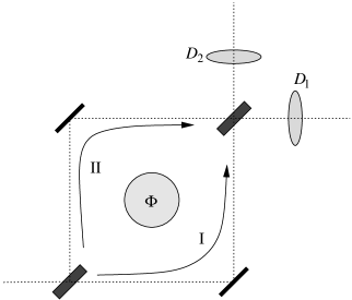
FIG. 5.: The Aharonov-Bohm effect in the setup of the Mach-Zender interferometer: the presence of $\Phi$ contributes to additional topological phase factors. Following path I gives rise to the factor $e^{i\lambda_{\text{I}}}$, and traversing path II yields $e^{i\lambda_{\text{II}}}$. The incoming particle still emerges at either detector $D_{1}$ or $D_{2}$, but the probabilities for either exit have been altered. The interference pattern now depends explicitly on the difference of the relative phases $e^{i\lambda}=e^{i(\lambda_{\text{I}}-\lambda_{\text{II}})}$.

The Mach-Zender apparatus is extended with a physical object $\Phi$ that we put at its center, as depicted in Fig. 5, and we assume that this object has a topological interaction with the injected particles. The incoming particle now acquires an additional phase factor which only depends on the topology of the path (where from a topological point of view $\Phi$ is a puncture of the two-dimensional plane). Paths I and II are topologically distinct and contribute the additional phase factors $e^{i\lambda_{\text{I}}}$ and $e^{i\lambda_{\text{II}}}$. The amplitude $A_{\text{AB}}[D_{1}]$ of the particle’s wave packet component at detector $D_{1}$ for the Aharonov-Bohm effect obviously includes these phase factors:

$$A_{\text{AB}}[D_{1}]=t_{1}r^{\prime}_{2}e^{i\theta_{\text{I}}}e^{i\lambda_{\text{I}}}+r_{1}t_{2}e^{i\theta_{\text{II}}}e^{i\lambda_{\text{II}}},$$ (18)

and likewise for the amplitude $A_{\text{AB}}[D_{2}]$ of the component at detector $D_{2}$.

The probabilities $P_{\text{AB}}[D_{i}]$ to observe a particle at either detector depend on the (gauge invariant) phase difference $e^{i(\lambda_{\text{I}}-\lambda_{\text{II}})}\equiv e^{i\lambda}$, which is the topological phase factor that a particle picks up when it circumvents $\Phi$ in a counterclockwise way. The probabilities $P_{\text{AB}}[D_{i}]$ are:

$$P_{\text{AB}}[D_{1}]=|t_{1}r^{\prime}_{2}|^{2}+|r_{1}t_{2}|^{2}+2Q\,\text{Re}\!\left(t_{1}r^{\prime}_{2}r^{*}_{1}t^{*}_{2}e^{i\theta}e^{i\lambda}\right),$$ (19)

$$P_{\text{AB}}[D_{2}]=|t_{1}t^{\prime}_{2}|^{2}+|r_{1}r_{2}|^{2}-2Q\,\text{Re}\!\left(t_{1}r^{\prime}_{2}r^{*}_{1}t^{*}_{2}e^{i\theta}e^{i\lambda}\right).$$ (20)

As expected, the particle still emerges from the apparatus with unit probability:

$$P_{\text{AB}}[D_{1}]+P_{\text{AB}}[D_{2}]=1.$$ (21)

We will use the above expressions for $P_{\text{AB}}[D_{i}]$ later on, where we also want to explicitly include the dependence on $e^{i\lambda}$. For this purpose we introduce $P_{e^{i\lambda}}[D_{i}]$, which is defined as:

$$P_{e^{i\lambda}}[D_{i}]\equiv P_{\text{AB}}[D_{i}].$$ (22)

The single particle run can be repeated for many particles, which gives rise to the interference patterns $I_{\text{AB}}[D_{i}]$ similar to those of eq. (13). And again, when the number $n$ of particles grows, the interference patterns approach the probability distributions:

$$\lim_{n\to\infty}I_{\text{AB}}[D_{1}]=P_{\text{AB}}[D_{1}]=P_{e^{i\lambda}}[D_{1}],$$ (23)

$$\lim_{n\to\infty}I_{\text{AB}}[D_{2}]=P_{\text{AB}}[D_{2}]=P_{e^{i\lambda}}[D_{2}].$$ (24)

This is about all there is to say about the Aharonov-Bohm interference experiment apart from an example that demonstrates how $e^{i\lambda}$ changes the interference pattern. Let us substitute $e^{i\lambda}=-1$ and the values from (16) into (19) and (20); this yields:

$$P_{\text{AB}}[D_{1}]=\frac{1}{10}\quad\quad P_{\text{AB}}[D_{2}]=\frac{9}{10},$$ (25)

where the particle is now with 90% chance detected by detector $D_{2}$ in contrast with the values of the probabilities in the example of the ordinary interference experiment given by (17).

C The setup with non-abelian anyons

The setup for - what up to now should be considered thought experiments with non-abelian anyons using the Mach-Zender interferometer, is very similar to the Aharonov-Bohm effect. The incoming particle will be a non-abelian anyon and the object $\Phi$ at the center of the apparatus will be replaced by another particle which is also a non-abelian anyon. So, it is no longer a single particle problem (one particle scattering of an invariant external object $\Phi$), but a two particle problem (one particle scattering of another one, both being non-abelian anyons). We will designate the incident non-abelian anyon as particle $B$ and the non-abelian anyon fixed at the apparatus’ center as particle $A$. The idea of the experiment remains the same as for the conventional interference experiments: we inject the particle $B$, in the Mach-Zender apparatus and detect it again with one of the two detectors $D_{1}$ and $D_{2}$, also see Fig. 6.

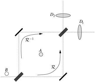
FIG. 6.: The setup for interference experiments with non-abelian anyons using the Mach-Zender interferometer. At the center of the apparatus resides a non-abelian anyon, particle $A$. The non-abelian anyon incident from the left is particle $B$. The non-abelian anyons have a topological interaction; if particle $B$ traverses the counterclockwise path this corresponds to the braid operator ${\cal R}$ acting on the two-particle internal state, the clockwise path yields the inverse operation ${\cal R}^{-1}$. The probabilities to emerge at detector $D_{1}$ and $D_{2}$ will explicitly depend on the expectation value of the monodromy operator ${\cal R}^{2}$.

In calculating the amplitudes and probabilities for the non-abelian anyon experiment we have to include the two-particle internal state $|\psi\rangle$, which is an element of the tensor product of the internal spaces $V^{B}$ and $V^{A}$ of particles $B$ and $A$:

$$|\psi\rangle\in V^{B}\otimes V^{A}$$ (26)

. The topological phase factors in the Aharonov-Bohm effect will be replaced by braid operators acting on the state $|\psi\rangle$. If particle $B$ follows path I within the apparatus it picks up a counterclockwise braid on the two-particle internal state: ${\cal R}|\psi\rangle$; if particle $B$ would traverse path II this would correspond to a clockwise braid: ${\cal R}^{-1}|\psi\rangle$.

Let us write down the amplitudes $A_{\text{NA}}[D_{i}]$ for the interference experiment with non-abelian anyons:

$$A_{\text{NA}}[D_{1}]=t_{1}r^{\prime}_{2}e^{i\theta_{\text{I}}}{\cal R}|\psi\rangle+r_{1}t_{2}e^{i\theta_{\text{II}}}{\cal R}^{-1}|\psi\rangle,$$ (27)

$$A_{\text{NA}}[D_{2}]=t_{1}t^{\prime}_{2}e^{i\theta_{\text{I}}}{\cal R}|\psi\rangle+r_{1}r_{2}e^{i\theta_{\text{II}}}{\cal R}^{-1}|\psi\rangle.$$ (28)

In calculating the probability distributions $P_{\text{NA}}[D_{i}]$, we use that the braid operators are unitary and $|\psi\rangle$ is properly normalized:

$$P_{\text{NA}}[D_{1}]=|t_{1}r^{\prime}_{2}|^{2}+|r_{1}t_{2}|^{2}+2Q\,\text{Re}\!\left(t_{1}r^{\prime}_{2}r^{*}_{1}t^{*}_{2}e^{i\theta}\langle\psi|{\cal R}^{2}|\psi\rangle\right),$$ (29)

$$P_{\text{NA}}[D_{2}]=|t_{1}t^{\prime}_{2}|^{2}+|r_{1}r_{2}|^{2}-2Q\,\text{Re}\!\left(t_{1}r^{\prime}_{2}r^{*}_{1}t^{*}_{2}e^{i\theta}\langle\psi|{\cal R}^{2}|\psi\rangle\right).$$ (30)

Compared with the probabilities $P_{\text{AB}}[D_{i}]$ for the Aharonov-Bohm effect, equations (19) and (20), the topological phase factor $e^{i\lambda}$ has been replaced by the expectation value $\langle\psi|{\cal R}^{2}|\psi\rangle$ of the monodromy operator ${\cal R}^{2}$ in (29) and (30).

We can re-write the probabilities $P_{\text{NA}}[D_{i}]$ when we use that the monodromy operator is unitary and thus has eigenvalues of the form $e^{i\lambda}$. If we introduce the projection operators $E_{\lambda}$ which project onto the eigenspace of $e^{i\lambda}$, we have that:

$${\cal R}^{2}=\sum_{\lambda}e^{i\lambda}E_{\lambda},\quad\quad p_{\lambda}\equiv\langle\psi|E_{\lambda}|\psi\rangle,$$ (31)

$$\langle\psi|{\cal R}^{2}|\psi\rangle=\sum_{\lambda}p_{\lambda}e^{i\lambda},\quad\quad\sum_{\lambda}E_{\lambda}=\openone,\quad\quad\sum_{\lambda}p_{\lambda}=1,$$ (32)

where we indicated the real-valued expectation value of $E_{\lambda}$ by $p_{\lambda}$. With eq. (22) in mind, the probability distribution of (29) can now be cast in the following form:

$$P_{\text{NA}}[D_{1}] = |t_{1}r^{\prime}_{2}|^{2}+|r_{1}t_{2}|^{2}+2Q\,\text{Re}\!\,\Bigl{(}t_{1}r^{\prime}_{2}r^{*}_{1}t^{*}_{2}e^{i\theta}\sum_{\lambda}p_{\lambda}e^{i\lambda}\Bigr{)}$$ (33)

$$= \sum_{\lambda}p_{\lambda}\Bigl{[}|t_{1}r^{\prime}_{2}|^{2}+|r_{1}t_{2}|^{2}+2Q\,\text{Re}\!\left(t_{1}r^{\prime}_{2}r^{*}_{1}t^{*}_{2}e^{i\theta}e^{i\lambda}\right)\Bigr{]}$$ (34)

$$= \sum_{\lambda}p_{\lambda}P_{e^{i\lambda}}[D_{1}].$$ (35)

This equation is nice because it gets rid of the uninteresting coefficients $r_{i}$,$Q$, etc; it states that the probability to observe particle $B$ at detector $D_{1}$ is a sum over probabilities of the Aharonov-Bohm version of the experiment, where the eigenvalues $e^{i\lambda}$ of the monodromy operator ${\cal R}^{2}$ play the role of the topological phase factor. The weight $p_{\lambda}$ in the sum is precisely the same weight as in the decomposition of (32) of $\langle\psi|{\cal R}^{2}|\psi\rangle$ into eigenvalues $e^{i\lambda}$. Of course, there is a similar decomposition for $P_{\text{NA}}[D_{2}]$, so we can write for $P_{\text{NA}}[D_{i}]$:

$$P_{\text{NA}}[D_{i}]=\sum_{\lambda}p_{\lambda}P_{e^{i\lambda}}[D_{i}],$$ (36)

and the total probability still equals unity:

$$P_{\text{NA}}[D_{1}]+P_{\text{NA}}[D_{2}]=\sum_{j,\lambda}p_{\lambda}P_{e^{i\lambda}}[D_{j}]=1.$$ (37)

Clearly, the values of the probabilities $P_{\text{NA}}[D_{i}]$ depend on the two-particle internal state $|\psi\rangle$, via the weights $p_{\lambda}$. Let us give an example to illustrate this. We plug the coefficients of the Mach-Zender apparatus given by (16) into eq. (36), and assume that the monodromy operator ${\cal R}^{2}$ has two eigenvalues: $\!+1,-1$ (eq. (97) shows a specific example of such a matrix ${\cal R}^{2}$). In the following table, we have given $P_{\text{NA}}[D_{i}]$ for three internal states, each of which is characterized by the $p_{\lambda}$; we also included the expectation value $\langle\psi|{\cal R}^{2}|\psi\rangle$.

			Probability distributions
.$p_{1}$	$p_{-1}$	$\langle\psi|{\cal R}^{2}|\psi\rangle$	$P_{\text{NA}}[D_{1}]$	$P_{\text{NA}}[D_{2}]$
.$\frac{1}{2}$	$\frac{1}{2}$	$0$	$\frac{1}{2}$	$\frac{1}{2}$
.$1$	$0$	$1$	$\frac{9}{10}$	$\frac{1}{10}$
.$0$	$1$	$-1$	$\frac{1}{10}$	$\frac{9}{10}$

It is worth mentioning that one is not restricted to the Mach-Zender interferometer to make the decomposition of the probabilities, like in expression (36). This is not so strange, since any dependence on the Mach-Zender apparatus, i.e., the coefficients $r_{i}$,$Q$ etc., is absent in (36). For instance, for double slit or plain scattering interference experiments with non-abelian anyons one can write down a similar decomposition. However, it is not conventional to do so; one usually keeps the expectation value of ${\cal R}^{2}$ explicit in one’s expressions.

D From probabilities to interference patterns

The interference experiment with non-abelian anyons is obviously a generalization of the Aharonov-Bohm experiment, by replacing the phase factor $e^{i\lambda}$ by a unitary operator ${\cal R}^{2}$, which has eigenvalues of the form $e^{i\lambda}$. But the picture of the interference experiment with non-abelian anyons is not complete yet, and requires further analysis. We have to consider the question of interference patterns, which for the case of non-abelian anyons we avoided so far.

What one wants is, to predict what one would observe in a realistic experiment. The interference pattern is the number of particles the detectors count if the experiment is repeated with many particles. For the ordinary interference and the Aharonov-Bohm experiments, is was perfectly legitimate to identify the interference patterns with the probability distributions, since by definition these are equal when the same experiment is repeated many times. Is this also true for the experiment with non-abelian anyons? The answer to this question turns out to be: not necessarily. The problem lies in the definition: in order to be the same one needs to repeat exactly the same experiment. For the non-abelian anyons experiment, this would imply that for each consecutive run, both particle $A$ and $B$ would have to be discarded, to be replaced by new particles $A$ and $B$, as is also shown in Fig. 7.

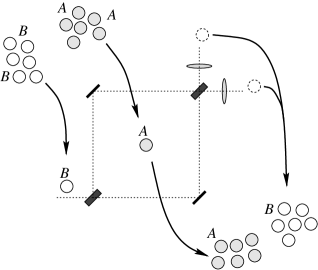
FIG. 7.: The many-to-many experiment. To be able to measure the initial probability distribution as the interference patterns requires that exactly the same run be repeated often. This means that after each observation of particle $B$ at either detector both particles $A$ and $B$ have to be replaced by new ones having the same initial internal state. The old particles cannot be re-used because the detection of particle $B$ at $D_{i}$ causes a change in the internal state. This way to repeat the runs is called the many-to-many experiment as it involves many particles $B$ and many particles $A$.

Why do we need a new particle $A$ and the same particle $B$ each time, why not use the old particles? The answer is, the two-particle internal state $|\psi\rangle$ not only affects the probabilities to observe particle $B$ at either detector, but is also altered itself by the detection, becoming a new, different state $|\psi^{\prime}\rangle$! It is obvious that an experiment with the internal state $|\psi\rangle$ gives another result than an experiment with internal state $|\psi^{\prime}\rangle$; so indeed, if we want to find the calculated probabilities as the observed interference pattern, we need a large supply of particles $A$ and $B$, all with the same internal states $|\psi\rangle$. Then we have that:

$$\lim_{n\to\infty}I^{\text{m-m}}_{\text{NA}}[D_{i}]=\lim_{n\to\infty}\frac{\#[D_{i}]}{n}=P_{\text{NA}}[D_{i}],$$ (38)

where $I^{\text{m-m}}_{\text{NA}}[D_{i}]$ indicate the interference patterns for the experiment with non-abelian anyons that is repeated with many particles $B$ directed to many particles $A$. We will refer to this type of experiment as a many-to-many (m-m) experiment.

However, we may decide to repeat the experiment in a different way, i.e., not using a new $A$ and $B$ each time, but then we will have to include the change in the internal state. The change in the two-particle internal state from $|\psi\rangle$ to $|\psi^{\prime}\rangle$ itself is also worth examining, and observable as well; if we want to observe the effect of this change of $|\psi\rangle$, it is necessary that we repeat the experiment while keeping at least one of the two old particles $A$ and $B$. We will discuss two such ways to repeat the experiment. First we will describe an experiment in which we keep using the same particle $A$ and particle $B$ for all consecutive runs, we call this the one-to-one experiment. The second way to repeat the experiment, is to keep only particle $A$ and replace each particle $B$ by a new one for each run; we will call this type of experiment many-to-one.

The reason that the two-particle internal state $|\psi\rangle$ gets changed, is because the detection of particle $B$ is a quantum mechanical measurement; there are two components of the two-particle wave packet, one associated with detector $D_{1}$, the other with $D_{2}$, and the measurement process projects out one of these components. The amplitudes $A_{\text{NA}}[D_{i}]$, (27) and (28), describe these components: the $D_{1}$ component is $t_{1}r^{\prime}_{2}e^{i\theta_{\text{I}}}{\cal R}|\psi\rangle+r_{1}t_{2}e^{i\theta_{\text{II}}}{\cal R}^{-1}|\psi\rangle$ and the $D_{2}$ component is $t_{1}t^{\prime}_{2}e^{i\theta_{\text{I}}}{\cal R}|\psi\rangle+r_{1}r_{2}e^{i\theta_{\text{II}}}{\cal R}^{-1}|\psi\rangle$. If particle $B$ is detected by $D_{1}$ the two-particle internal state $|\psi\rangle$ changes to $|\psi^{\prime}\rangle$, which is the normalized $D_{1}$ component:

$$|\psi^{\prime}\rangle=\frac{1}{\sqrt{K}}\left(t_{1}r^{\prime}_{2}e^{i\theta_{\text{I}}}{\cal R}|\psi\rangle+r_{1}t_{2}e^{i\theta_{\text{II}}}{\cal R}^{-1}|\psi\rangle\right),$$ (39)

where the real factor $K$ is the normalization constant. There is a similar expression for the case particle $B$ is detected by detector $D_{2}$.

A priori, we may not assume that we know the precise values of $t_{i}$, $r_{i}$, $r^{\prime}_{i}$, $e^{i\theta_{\text{I}}}$, $e^{i\theta_{\text{II}}}$ in the above expression (39); it is also doubtful whether we know $|\psi\rangle$ beforehand, but even if we do, we know little of the new state $|\psi^{\prime}\rangle$. The best we can say is that $|\psi^{\prime}\rangle$ will be an entangled state, i.e., it cannot be factorized as a simple tensor product $|x\rangle\otimes|y\rangle$, $|x\rangle\in V^{A}$, $|y\rangle\in V^{B}$; this is because $|\psi^{\prime}\rangle$ is, see eq. (39), some linear combination of ${\cal R}$ and ${\cal R}^{-1}$ acting on $|\psi\rangle$, and for non-trivial ${\cal R}$ and ${\cal R}^{-1}$ this action usually results in entanglement, independent of whether the initial state $|\psi\rangle$ was entangled. However, as we will see in the one-to-one and the many-to-one experiment, it turns out that we can work with this expression for $|\psi^{\prime}\rangle$ and eventually, after observing many incident particles at the detectors, we can even determine $|\psi^{\prime}\rangle$ with precision.

III The inequivalent classes of interference experiments

In this section we want to consider the various possibilities for the interference experiments in detail. We start with the one-to-one experiment followed by the many-to-one experiment (we already discussed the many-to-many experiment in the previous section). We conclude by summarizing the different results in a Table IV .

A The one-to-one experiment

The one-to-one experiment requires only one particle $A$ and one particle $B$. What we will show in this subsection, is that after repeating the one-to-one experiment a sufficient number of times, the system will get locked into an eigenstate of the monodromy operator ${\cal R}^{2}$ with a probability determined by the initial state. We inject particle $B$ at the left of the Mach-Zender apparatus, with particle $A$ at its center, and detect particle $B$ at detector $D_{1}$ or $D_{2}$, and we repeat this procedure using the same particles $B$ and $A$. This of course requires, that we route particle $B$ back to its original position - the entrance point at the left of the apparatus. We assume that we can extend the Mach-Zender device with some additional mirrors that take care of this, as depicted in Fig. 8. As we move non-abelian anyons around, we should be aware that this may include some action of the braid operators; as we move particle $B$ back, we exchange it with particle $A$ in a counterclockwise way, which means that an additional braid operation ${\cal R}$ acts on the two-particle internal state $|\psi^{\prime}\rangle$.

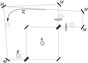
FIG. 8.: The setup for the one-to-one experiment, which uses only one particle $B$ and one particle $A$. Additional (intelligent) mirrors $M$ have been placed around the Mach-Zender device to route particle $B$ back to its original position after it has been detected by $D_{1}$ or $D_{2}$, where it will be injected again in the apparatus. As particle $B$ is returned, it passes particle $A$ in a counterclockwise fashion, which means the braid operator ${\cal R}$ should act on the two-particle internal state. Particle $A$ remains all the time unperturbed at the center of the apparatus. With each detection of particle $B$, the two-particle internal state may change.

Let us take a closer look at the one-to-one experiment, paying special attention to the internal state. We start with an initial two-particle internal state $|\psi\rangle\equiv|\psi_{0}\rangle$, and insert particle $B$ in the apparatus. We then observe particle $B$ at one of the detectors $D_{i}$. The probability to emerge at detector $D_{i}$ is of course given by (29): $P_{\text{NA}}[D_{i}]=P_{\text{NA}}[D_{i}]_{|\psi_{0}\rangle}$, to show explicitly the dependence on the internal state $|\psi_{0}\rangle$. Since the probability for each detector will in general be non-zero, there are two possible outcomes for the first run: particle $B$ is detected at $D_{1}$ or at $D_{2}$. If it is at detector $D_{1}$ and we return particle $B$ to its initial position, the new two-particle internal state $|\psi_{1}\rangle$ (we will use $|\psi_{j}\rangle$ to indicate the internal state after the $j$th run) will be:

$$|\psi_{1}\rangle = {\cal R}\frac{1}{\sqrt{K}}\left(t_{1}r^{\prime}_{2}e^{i\theta_{\text{I}}}{\cal R}|\psi\rangle+r_{1}t_{2}e^{i\theta_{\text{II}}}{\cal R}^{-1}|\psi\rangle\right)$$ (40)

$$= \frac{1}{\sqrt{K}}\left(t_{1}r^{\prime}_{2}e^{i\theta_{\text{I}}}{\cal R}^{2}+r_{1}t_{2}e^{i\theta_{\text{II}}}\openone\right)|\psi_{0}\rangle.$$ (41)

If we would find particle $B$ at detector $D_{2}$, the new state $|\psi_{1}\rangle$ would be:

$$|\psi_{1}\rangle=\frac{1}{\sqrt{K^{\prime}}}\left(t_{1}t^{\prime}_{2}e^{i\theta_{\text{I}}}{\cal R}^{2}+r_{1}r_{2}e^{i\theta_{\text{II}}}\openone\right)|\psi_{0}\rangle,$$ (42)

where $K^{\prime}$ is a normalization constant that will in general be different from $K$.

We can easily continue this for a second run. The probability to observe particle $B$ at detector $D_{i}$ at the second run is given by $P_{\text{NA}}[D_{i}]_{|\psi_{1}\rangle}$, where we note that $|\psi_{1}\rangle$, albeit implicitly, depends on the outcome of the first run. Of course, there are two possible outcomes for the second run, and the resulting internal state $|\psi_{2}\rangle$ will depend on the outcomes of the first and second run. We could follow this procedure for a large number of runs, say $n$. However, this means we would have to work with an internal state $|\psi_{n}\rangle$ depending on the outcomes of all $n$ runs, meaning there would be $2^{n}$ possible outcomes to consider! Although this would probably lead to the correct answer, the number $2^{n}$ grows so incredibly fast, that this way is not advisable, and indeed we will follow another path to the answer.

We are basically interested in two things after we repeated the experiment for $n$ runs: firstly the interference pattern, i.e., how many times $\#[D_{i}]$ out of the total $n$ we observed the incident particle at detector $D_{i}$, and secondly, what we can say about the internal state $|\psi_{n}\rangle$ given the interference pattern.

The interference pattern has something to do with the probabilities $P_{\text{NA}}[D_{i}]_{|\psi_{j}\rangle}$, $j=1,2,\ldots,n$. Since $|\psi_{1}\rangle$ is different from $|\psi_{0}\rangle$, which is in the general case true and independent of the outcome of the first run, we can write down the following inequality concerning their probability distributions:

$$P_{\text{NA}}[D_{i}]_{|\psi_{1}\rangle}\neq P_{\text{NA}}[D_{i}]_{|\psi_{0}\rangle}.$$ (43)

One can wonder if such an inequality holds also for the $j$th and $(j+1)$th run. This would mean that the probabilities keep fluctuating from run to run and the resulting interference pattern would become random, and thereby also independent on the initial internal state $|\psi_{0}\rangle$. However, it turns out that this is not so, and after a large number of runs the inequality of (43) converges to an equality:

$$P_{\text{NA}}[D_{i}]_{|\psi_{n+1}\rangle}=P_{\text{NA}}[D_{i}]_{|\psi_{n}\rangle}\quad\text{for }n\to\infty.$$ (44)

The equality in (44) is automatically satisfied if $|\psi_{n+1}\rangle$ and $|\psi_{n}\rangle$ would differ only by a phase factor, i.e.:

$$|\psi_{n+1}\rangle=e^{i\alpha}|\psi_{n}\rangle\quad\text{for arbitrary }e^{i\alpha}.$$ (45)

There is a class of internal states that obey eq. (45): the eigenstates of the monodromy operator ${\cal R}^{2}$. If $|\psi_{n}\rangle$ would be an eigenstate of ${\cal R}^{2}$ with eigenvalue $e^{i\lambda}$ then, after the $(n+1)$th run, the internal state $|\psi_{n+1}\rangle$ would be, according to (41) if the outcome of the $n$th run had been observation at detector $D_{1}$:

$$|\psi_{n+1}\rangle=e^{i\alpha}|\psi_{n}\rangle,\quad e^{i\alpha}=\frac{1}{\sqrt{K}}\left(t_{1}r^{\prime}_{2}e^{i\theta_{\text{I}}}e^{i\lambda}+r_{1}t_{2}e^{i\theta_{\text{II}}}\right).$$ (46)

If at the $(n+1)$th run, particle $B$ was found at detector $D_{2}$, the new internal state would have been, using (42):

$$|\psi_{n+1}\rangle=e^{i\alpha^{\prime}}|\psi_{n}\rangle,\quad e^{i\alpha^{\prime}}=\frac{1}{\sqrt{K^{\prime}}}\left(t_{1}t^{\prime}_{2}e^{i\theta_{\text{I}}}e^{i\lambda}+r_{1}r_{2}e^{i\theta_{\text{II}}}\right).$$ (47)

The probability distributions $P_{\text{NA}}[D_{i}]_{|\psi_{n}\rangle}$ indeed turn out to converge to a fixed value that is associated with an eigenvalue $e^{i\lambda}$ of the monodromy operator, when the number of runs $n$ becomes large, i.e.:

$$\lim_{n\to\infty}P_{\text{NA}}[D_{1}]_{|\psi_{n}\rangle}=|t_{1}r^{\prime}_{2}|^{2}+|r_{1}t_{2}|^{2}+2Q\,\text{Re}\!\left(t_{1}r^{\prime}_{2}r^{*}_{1}t^{*}_{2}e^{i\theta}e^{i\lambda}\right).$$ (48)

In eq. (48) we still used the notation that includes the Mach-Zender apparatus’ coefficients; let us write (48) in the preferred device independent notation:

$$\lim_{n\to\infty}P_{\text{NA}}[D_{i}]_{|\psi_{n}\rangle}=P_{e^{i\lambda}}[D_{i}].$$ (49)

It is not only the probability distributions that converge, for the internal state $|\psi_{n}\rangle$ also becomes fixed: as the eigenstate of ${\cal R}^{2}$ that carries the eigenvalue $e^{i\lambda}$, in other words:

$$\lim_{n\to\infty}\langle\psi_{n}|{\cal R}^{2}|\psi_{n}\rangle=e^{i\lambda}$$ (50)

So, we conclude that the internal state is locked into an eigenstate of ${\cal R}^{2}$; the only change subsequent runs of the experiment can accomplish, is an uninteresting overall phase factor $e^{i\alpha}$, as follows from (46) and (47).

But ${\cal R}^{2}$ has in general more than one eigenvalue. What can we say about which eigenvalue $e^{i\lambda}$ will come out, i.e., to which eigenvalue and eigenstate do $P_{NA}[D_{i}]_{|\psi_{n}\rangle}$ and $|\psi_{n}\rangle$ will converge? This is where the initial internal state $|\psi\rangle=|\psi_{0}\rangle$ comes in; if the expectation value of ${\cal R}^{2}$ and $|\psi\rangle$ is given by:

$$\langle\psi|{\cal R}^{2}|\psi\rangle=\sum_{\lambda}p_{\lambda}e^{i\lambda},$$ (51)

then the probability that the two particle system gets locked in the eigenstate of $e^{i\lambda}$ is given by $p_{\lambda}$.

We will now consider the actual interference pattern $I^{\text{o-o}}_{\text{NA}}[D_{i}]$ of the one-to-one (o-o) experiment with non-abelian anyons and argue that it equals the fixed probability distribution of (49). Let us assume that projection, i.e., locking, is not achieved until the $m$th run. Then the outcomes of the first $m$ runs were governed by other probabilities than of eq. (49) and the interference pattern, i.e., the collection of outcomes at the time of the $m$th run, will not look like (49). However, after the $m$th run, we can repeat the experiment for an additional $n$ runs, where $n$ can be much greater than $m$; all these subsequent outcomes will obey (49) and, since $n\gg m$, completely dominate the interference pattern, rendering the first $m$ contributions negligible:

$$\lim_{n\to\infty}I^{\text{o-o}}_{\text{NA}}[D_{i}]=P_{e^{i\lambda}}[D_{i}].$$ (52)

Not only does the monodromy operator ${\cal R}^{2}$ in general have multiple distinct eigenvalues, these eigenvalues can be degenerate as well. This degeneracy has no effect on the resulting interference pattern, which remains of the form of (52). However, the internal state does not become projected onto a particular eigenstate, but rather onto the eigenspace of eigenvalue $e^{i\lambda}$:

$$\lim_{n\to\infty}|\psi_{n}\rangle=\frac{E_{\lambda}|\psi\rangle}{\sqrt{\langle\psi|E_{\lambda}|\psi\rangle}},$$ (53)

where the square root in the denominator is there to normalize the state; $E_{\lambda}$ is the projection operator projecting onto the eigenspace of $e^{i\lambda}$. The probability $p_{\lambda}$ can also be given in terms of the projection operator $E_{\lambda}$:

$$p_{\lambda}=\langle\psi|E_{\lambda}|\psi\rangle.$$ (54)

We have showed that eigenstates of the monodromy operator are fixed states, and said that all initial internal states eventually become locked. The complete (nontrivial) proof of this convergence of arbitrary initial states is rather lengthy, and we have relegated it to the Appendix.

Projection is achieved after a large but finite number of runs. How do we know when we have reached such a projected, fixed, state? This, we determine from the interference patterns: if we can identify the interference pattern $I_{\text{NA}}^{\text{o-o}}[D_{i}]$ with extreme certainty with one and only one $P_{e^{i\lambda}}[D_{i}]$, we know the state is projected onto the eigenspace of $e^{i\lambda}$. The harder it is to distinguish the $P_{e^{i\lambda}}[D_{i}]$ for different $e^{i\lambda}$, the longer (more runs) it takes before projection will be realized.

Let us conclude the one-to-one experiment with an example, with the same values (16) for the coefficients of the Mach-Zender interferometer, and a monodromy matrix ${\cal R}^{2}$ with eigenvalues $\pm 1$, as we used before. In the following table we give the interference patterns $I^{\text{o-o}}_{\text{NA}}[D_{i}]$ and their probability to come out of the experiment for four different initial internal states (which are characterized by $p_{1}$ and $p_{=-1}$). So, in this example, there are two possible observable interference patterns: either we observe nine out of ten times particle $B$ at detector $D_{1}$ and one out of ten at detector $D_{2}$ or the other way around (see the Table). Of the two situations we may end up with, we can only calculate the probabilities, as it should in this quantum mechanical setting.

.$p_{1}$	$p_{-1}$	$I^{\text{o-o}}_{\text{NA}}[D_{1}]$	$I^{\text{o-o}}_{\text{NA}}[D_{2}]$	Probability
.$\frac{1}{2}$	$\frac{1}{2}$	$\frac{9}{10}$	$\frac{1}{10}$	$\frac{1}{2}$
.		$\frac{1}{10}$	$\frac{9}{10}$	$\frac{1}{2}$
.$1$	$0$	$\frac{9}{10}$	$\frac{1}{10}$	$1$
.$0$	$1$	$\frac{1}{10}$	$\frac{9}{10}$	$1$
.$\frac{3}{8}$	$\frac{5}{8}$	$\frac{9}{10}$	$\frac{1}{10}$	$\frac{3}{8}$
.		$\frac{1}{10}$	$\frac{9}{10}$	$\frac{5}{8}$

B The many-to-one experiment: probe one particle with many others

In the many-to-one experiment, the experiment is repeated with the same particle $A$ but with a new particle $B$ each time. This will lead to a different result, for now the system will get locked into an eigenstate of a different operator called $U$, which will be defined below.

The setup of the Mach-Zender apparatus in this case no longer requires the extension with mirrors as needed for the one-to-one experiment, but it does require a large supply, i.e., a ‘bag’ with many identical particles $B$ in it, on the left of the apparatus, see Fig. 9. We will be using the notation/convention for braids of these multiple particles as we introduced in section I (i.e. writing particles left in the experiment left in the tensor product, ${\cal R}_{i}$ interchanging particles $i$ and $(i+1)$ anticlockwise, numbering form right to left beginning with one). The total system’s initial internal state $|\psi\rangle$ is an element of the tensor product of the internal spaces $V^{B}$ of the $B$ particles and $V^{A}$ of the $A$ particle:

$$|\psi\rangle\in V^{B}\otimes\cdots\otimes V^{B}\otimes V^{B}\otimes V^{B}\otimes V^{A}.$$ (55)

Once a $B$ particle has been used, it has become uninteresting but we will not discard it completely, merely collect such $B$ particles somewhere on the right of the apparatus.

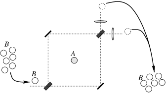
FIG. 9.: The many-to-one experiment: the same particle $A$ remains continuously at the center of the apparatus during the experiment, but particle $B$ gets replaced by a new one after detection. All $B$ particles initially carry the same internal state. The multi-particle internal state changes with each observation of the current particle $B$ at detector $D_{1}$ or $D_{2}$ and may become highly entangled.

For reasons of simplicity and to give a full solution, we will subject the internal state $|\psi\rangle$ to the following conditions: the initial internal state $|\psi\rangle$ should factorize completely, i.e., the initial internal state should be unentangled, and furthermore, the $B$ particles should have trivial braiding:

$${\cal R}_{i}|\psi\rangle={\cal R}^{-1}_{i}|\psi\rangle=\sigma_{i}|\psi\rangle=|\psi\rangle\quad\quad\forall\,i\geq 2,$$ (56)

where $\sigma_{i}$ is the operator that only swaps particle $i$ and $(i+1)$ without affecting their internal state. Applying both conditions to the internal state $|\psi\rangle$, implies that $|\psi\rangle$ can be written in the following form:

$$|\psi\rangle=y^{i_{n}}\ldots y^{i_{2}}y^{i_{1}}x^{\alpha}|e_{i_{n}}\rangle\ldots|e_{i_{2}}\rangle|e_{i_{1}}\rangle|f_{\alpha}\rangle,$$ (57)

where $\{|e_{i_{j}}\rangle\}$is a basis for the internal space $V^{B}$ of the $j$th particle $B$, and $\{|f_{\alpha}\rangle\}$ a basis for $V^{A}$.

Let us start the first run of the thought experiment: we insert the first particle $B$ in the Mach-Zender interferometer and observe it again at either detector $D_{1}$ or $D_{2}$. The probabilities $P_{\text{NA}}[D_{i}]$ for detector $D_{i}$ are of course given by (35), (36), and depend on the expectation value $\langle\psi_{0}|{\cal R}^{2}_{1}|\psi_{0}\rangle$ of the monodromy operator ${\cal R}^{2}_{1}$ which acts on particle $A$ and the first particle $B$, with respect to the initial internal state $|\psi_{0}\rangle\equiv|\psi\rangle$. Let us assume we observe the first incident particle at detector $D_{1}$, then the new, changed, internal state, which we indicate by $|\psi_{1}\rangle$, is given by:

$$|\psi_{1}\rangle=\frac{1}{\sqrt{K}}\left(t_{1}r^{\prime}_{2}e^{i\theta_{\text{I}}}{\cal R}_{1}+r_{1}t_{2}e^{i\theta_{\text{II}}}{\cal R}^{-1}_{1}\right)|\psi_{0}\rangle.$$ (58)

Because the first particle $B$ is now to the right of particle $A$, the new internal state $|\psi_{1}\rangle$ is strictly speaking an element of a different vector space than that of $|\psi_{0}\rangle$:

$$|\psi_{1}\rangle\in V^{B}\otimes\cdots\otimes V^{B}\otimes V^{B}\otimes V^{A}\otimes V^{B}.$$ (59)

Furthermore, the first particle $B$ and particle $A$ are now entangled, so the internal state $|\psi_{1}\rangle$ cannot be completely factorized anymore:

$$|\psi_{1}\rangle=y^{i_{n}}\ldots y^{i_{2}}z^{\alpha i_{1}}|e_{i_{n}}\rangle\ldots|e_{i_{2}}\rangle|f_{\alpha}\rangle|e_{i_{1}}\rangle,$$ (60)

where the components $z^{\alpha i_{1}}$ are determined by the coefficients of (58) and the components $x^{\alpha}$ and $y^{i}$. The second up to the $n$th $B$ particle, still have trivial braiding, which we can generalize to the $j$th run of the experiment by the statement:

$${\cal R}_{i}|\psi_{j}\rangle=|\psi_{j}\rangle,\quad\quad i>j+1.$$ (61)

So far for the first run.

For the second run, the next particle $B$ is injected in the Mach-Zender apparatus, and the probabilities to observe it at detector $D_{i}$ are now governed by the expectation value $\langle\psi_{1}|{\cal R}_{2}^{2}|\psi_{1}\rangle$ of the current internal state $|\psi_{1}\rangle$ and the monodromy operator ${\cal R}_{2}^{2}$ that operates on particle $A$ and the second particle $B$. This expectation value will in general be different from the expectation value of the first run: $\langle\psi_{1}|{\cal R}_{2}^{2}|\psi_{1}\rangle\neq\langle\psi_{0}|{\cal R}_{1}^{2}|\psi_{0}\rangle$, and thus the probabilities for the first and second run will be different. But, just as in the case of the one-to-one experiment, the probabilities and thus the expectation values will converge to a final, fixed, value:

$$\langle\psi_{n+1}|{\cal R}_{n+2}^{2}|\psi_{n+1}\rangle=\langle\psi_{n}|{\cal R}_{n+1}^{2}|\psi_{n}\rangle,\quad\quad n\to\infty.$$ (62)

We would like to know which states obey this equality (62) and what the expectation value will be. These will not be eigenstates and eigenvalues of a monodromy operator, as for the one-to-one experiment, but something related.

Let us now start solving equation (62) if we assume that the $(n+1)$th particle $B$ has been observed at detector $D_{1}$, and use that we know $|\psi_{n+1}\rangle$ in terms of $|\psi_{n}\rangle$, as in (58):

$$\langle\psi_{n+1}|{\cal R}_{n+2}^{2}|\psi_{n+1}\rangle = \frac{1}{K}\biggl{(}\,|t_{1}r^{\prime}_{2}|^{2}\langle\psi_{n}|{\cal R}^{-1}_{n+1}{\cal R}^{2}_{n+2}{\cal R}_{n+1}|\psi_{n}\rangle+t_{1}r^{\prime}_{2}r_{1}^{*}t_{2}^{*}e^{i(\theta_{\text{I}}-\theta_{\text{II}})}\langle\psi_{n}|{\cal R}_{n+1}{\cal R}^{2}_{n+2}{\cal R}_{n+1}|\psi_{n}\rangle$$ (64)

$$\quad\quad+|r_{1}t_{2}|^{2}\langle\psi_{n}|{\cal R}_{n+1}{\cal R}^{2}_{n+2}{\cal R}^{-1}_{n+1}|\psi_{n}\rangle+t_{1}^{*}r^{\prime*}_{2}r_{1}t_{2}e^{-i(\theta_{\text{I}}-\theta_{\text{II}})}\langle\psi_{n}|{\cal R}^{-1}_{n+1}{\cal R}^{2}_{n+2}{\cal R}^{-1}_{n+1}|\psi_{n}\rangle\biggr{)}$$

$$= \langle\psi_{n}|{\cal R}_{n+1}^{2}|\psi_{n}\rangle,$$ (65)

where the normalization constant $K$ is given by:

$$K=|t_{1}r^{\prime}_{2}|^{2}+|r_{1}t_{2}|^{2}+2\,\text{Re}\!\left(t_{1}r^{\prime}_{2}r_{1}^{*}t_{2}^{*}e^{i(\theta_{\text{I}}-\theta_{\text{II}})}\langle\psi_{n}|{\cal R}_{n+1}^{2}|\psi_{n}\rangle\right).$$ (66)

These two expressions, (64), (66), may look horrid (and we can write down another pair for the case that outcome of the $(n+1)$th run is observation at detector $D_{2}$), but they are not that bad if we apply the braid relations to them, i.e., use the fact that the ${\cal R}_{n}$ satisfy the Yang-Baxter relations. Using (61) as well, two of the four expectation values in (64) simplify to:

$$\langle\psi_{n}|{\cal R}^{-1}_{n+1}{\cal R}^{2}_{n+2}{\cal R}_{n+1}|\psi_{n}\rangle = \langle\psi_{n}|{\cal R}_{n+2}{\cal R}^{2}_{n+1}{\cal R}^{-1}_{n+2}|\psi_{n}\rangle$$ (67)

$$= \langle\psi_{n}|{\cal R}^{2}_{n+1}|\psi_{n}\rangle$$ (68)

$$\equiv \kappa,$$ (69)

$$\langle\psi_{n}|{\cal R}_{n+1}{\cal R}^{2}_{n+2}{\cal R}^{-1}_{n+1}|\psi_{n}\rangle = \langle\psi_{n}|{\cal R}^{-1}_{n+2}{\cal R}^{2}_{n+1}{\cal R}_{n+2}|\psi_{n}\rangle$$ (70)

$$= \langle\psi_{n}|{\cal R}^{2}_{n+1}|\psi_{n}\rangle$$ (71)

$$= \kappa,$$ (72)

where we introduced $\kappa$ to indicate the expectation value $\langle\psi_{n}|{\cal R}^{2}_{n+1}|\psi_{n}\rangle$. Equation (64) will be solved if $|\psi_{n}\rangle$ is such that:

$$\langle\psi_{n}|{\cal R}_{n+1}{\cal R}^{2}_{n+2}{\cal R}_{n+1}|\psi_{n}\rangle=\kappa^{2},$$ (73)

$$\langle\psi_{n}|{\cal R}^{-1}_{n+1}{\cal R}^{2}_{n+2}{\cal R}^{-1}_{n+1}|\psi_{n}\rangle=\kappa\kappa^{*}.$$ (74)

Let us rewrite these expectation values too, by applying then Yang-Baxter equation and eq. (61) once more:

$$\langle\psi_{n}|{\cal R}_{n+1}{\cal R}^{2}_{n+2}{\cal R}_{n+1}|\psi_{n}\rangle=\langle\psi_{n}|{\cal R}_{n+1}^{2}\sigma_{n+2}{\cal R}^{2}_{n+1}\sigma_{n+2}|\psi_{n}\rangle,$$ (75)

$$\langle\psi_{n}|{\cal R}^{-1}_{n+1}{\cal R}^{2}_{n+2}{\cal R}^{-1}_{n+1}|\psi_{n}\rangle=\langle\psi_{n}|{\cal R}_{n+1}^{-2}\sigma_{n+2}{\cal R}^{2}_{n+1}\sigma_{n+2}|\psi_{n}\rangle.$$ (76)

Although ${\cal R}_{n+1}^{2}$ and $\sigma_{n+2}{\cal R}^{2}_{n+1}\sigma_{n+2}$ are distinct operators, their matrix elements $(R^{2})^{i\alpha}_{j\beta}$ are equal:

$$(R^{2})^{i\alpha}_{j\beta}=\langle e^{i}|\langle f^{\alpha}|{\cal R}^{2}|e_{j}\rangle|f_{\beta}\rangle.$$ (77)

We will decompose the right hand side of (75) in a similar way in components relative to the bases $\{|e_{i}\rangle\}$, $\{|f_{\alpha}\rangle\}$ of the vector spaces $V^{B}$ and $V^{A}$. The internal state $|\psi_{n}\rangle$ decomposes as:

$$|\psi_{n}\rangle=y^{i}y^{j}z^{\alpha i_{n}\ldots i_{1}}|e_{i}\rangle|e_{j}\rangle|f_{\alpha}\rangle|e_{i_{n}}\rangle\ldots|e_{i_{1}}\rangle.$$ (78)

Next, we let the combined operators ${\cal R}_{n+1}^{2}$ and $\sigma_{n+2}{\cal R}^{2}_{n+1}\sigma_{n+2}$ act on a basis state (ignoring the $|e_{i_{n}}\rangle\ldots|e_{i_{1}}\rangle$ part) to give:

$${\cal R}_{n+1}^{2}\sigma_{n+2}{\cal R}^{2}_{n+1}\sigma_{n+2}|e_{i}\rangle|e_{j}\rangle|f_{\alpha}\rangle=(R^{2})^{k\beta}_{i\alpha}(R^{2})^{l\gamma}_{j\beta}|e_{k}\rangle|e_{l}\rangle|f_{\gamma}\rangle.$$ (79)

If we also introduce the density matrices $\rho_{A}$ and $\rho_{B}$ of particles $A$ and $B$:

$$(\rho_{A})^{\alpha}_{\beta}=z^{\alpha i_{n}\ldots i_{1}}z_{\beta i_{n}\ldots i_{1}},\quad\quad(\rho_{B})^{i}_{j}=y^{i}y_{j},$$ (80)

then the expectation value of (75) can be written as follows:

$$\langle\psi_{n}|{\cal R}_{n+1}^{2} \sigma_{n+2}{\cal R}^{2}_{n+1}\sigma_{n+2}|\psi_{n}\rangle=$$ (85)

$$=(R^{2})^{k\beta}_{i\alpha}(R^{2})^{l\gamma}_{j\beta}(\rho_{B})^{i}_{k}(\rho_{B})^{j}_{l}(\rho_{A})^{\alpha}_{\gamma}$$

$$=[(\rho_{B})^{j}_{l}(R^{2})^{l\gamma}_{j\beta}][(\rho_{B})^{i}_{k}(R^{2})^{k\beta}_{i\alpha}](\rho_{A})^{\alpha}_{\gamma}$$

$$=U^{\gamma}_{\beta}U^{\beta}_{\alpha}(\rho_{A})^{\alpha}_{\gamma}$$

$$=\text{Tr}(UU\rho_{A}).$$

Here, in the last two steps of eq. (85), we introduced – as announced – an operator $U$ that operates on $V^{A}$ and is defined as the partial trace over the $B$ space of the monodromy operator ${\cal R}^{2}$ and the density matrix of particle $B$:

$$U^{\alpha}_{\beta}=(\rho_{B})^{j}_{i}(R^{2})^{i\alpha}_{j\beta},\quad\quad U_{A}=\text{Tr}_{B}(\rho_{B}{\cal R}^{2}_{BA}).$$ (86)

Let us now reconsider our original problem in terms of the $U$ and $\kappa$. We can express $\kappa$ as the trace over $U$ and the density matrix of particle $A$:

$$\kappa=\text{Tr}(U\rho_{A}).$$ (87)

The condition to satisfy equality (64), as given by (73), becomes in terms of $U$:

$$\text{Tr}(U^{2}\rho_{A})=\kappa^{2}.$$ (88)

Since the trace of an operator and a density matrix can be regarded as the expectation value of that operator, we have that:

$$\langle U^{2}\rangle=\langle U\rangle^{2},$$ (89)

which can only be true if $\kappa$ is an eigenvalue of $U$ and $\rho_{A}$ lies in the eigenspace of the eigenvalue $\kappa$.

Just as in the one-to-one experiment, the probability distributions for the incident particles converge to a fixed distribution associated with the eigenvalue of an operator, and the final distribution determines the interference pattern. Also, the system becomes projected onto the eigenspace of the observed eigenvalue. However, the eigenvalues and eigenstates are no longer given by the monodromy operator ${\cal R}^{2}$ as in the one-to-one experiment; in the many-to-one (m-o) experiment we observe an eigenvalue $\kappa$ of the operator $U$ and have projection onto the eigenspace of that eigenvalue. If we denote the probability distributions by $P^{\text{m-o}}_{\text{NA}}[D_{i}]$, we see that for large $n$ they become equal to the interference patterns $I^{\text{m-o}}_{\text{NA}}[D_{i}]$ :

$$\lim_{n\to\infty}P^{\text{m-o}}_{\text{NA}}[D_{1}]_{|\psi_{n}\rangle} = \lim_{n\to\infty}I^{\text{m-o}}_{\text{NA}}[D_{1}]$$ (90)

$$= |t_{1}r^{\prime}_{2}|^{2}+|r_{1}t_{2}|^{2}+2Q\,\text{Re}\!\left(t_{1}r^{\prime}_{2}r^{*}_{1}t^{*}_{2}e^{i\theta}\kappa\right)$$ (91)

$$\equiv P_{\kappa}[D_{1}],$$ (92)

where we used $P_{\kappa}[D_{1}]$ to indicate the locked probability distribution that is associated with the eigenvalue $\kappa$; of course there are similar expressions for $D_{2}$. As far as the projection of the internal state is concerned, there is strictly speaking only a projection in a subsystem of the total system’s internal state, namely the subsystem describing the internal state of particle $A$, because $U$ acts on $V^{A}$ only. It is the density matrix of particle $A$ that becomes projected onto the associated eigenspace of $\kappa$:

$$\rho_{A}\to\frac{E_{\kappa}\rho_{A}E_{\kappa}}{\text{Tr}(E_{\kappa}\rho_{A})}\quad\quad\text{for }n\to\infty,$$ (93)

where $E_{\kappa}$ is the projection operator of the eigenspace of $\kappa$. Just as the monodromy operator ${\cal R}^{2}$ can have multiple (degenerate) eigenvalues, so can $U$. Each eigenvalue $\kappa$ has a probability $p_{\kappa}$ to be observed in the end; $p_{\kappa}$ is determined by the initial density matrix $\rho_{A}$:

$$p_{\kappa}=\text{Tr}(E_{\kappa}\rho_{A}),\quad\quad(\rho_{A})^{\alpha}_{\beta}=x^{\alpha}x_{\beta}.$$ (94)

Above, we have showed that there exist states for which the probability distributions are locked, and that there is a chance $p_{\kappa}$ to end up in each locked state. The proof of it is almost the same as that of the convergence in the one-to-one experiment and can be found in the Appendix.

To solve the many-to-one experiment we introduced two conditions: the initial internal state should factorize completely and the $B$ particles should have trivial braiding. We believe these conditions are too restrictive: the many-to-one experiment should be possible for arbitrary entangled initial states, subjected only to the condition that the $B$ particles have abelian braiding:

$${\cal R}_{j}|\psi_{k}\rangle=e^{is_{B}}|\psi_{k}\rangle\quad\quad j>k,$$ (95)

where the $s_{B}$ in the phase factor $e^{is_{B}}$ is also known as the spin of the $B$ particles. In this generalized many-to-one experiment, the interference patterns also depend explicitly on $\kappa$:

$$\lim_{n\to\infty}I^{\text{m-o}}_{\text{NA}}[D_{i}]=P_{\kappa}[D_{i}],$$ (96)

but $\kappa$ can no longer be regarded as the eigenvalue of the operator $U$; the definition of $U$ becomes ambiguous, because $U$ is the trace of ${\cal R}^{2}$ and the density matrix $\rho_{B}$ of the $B$ particles, and in this case $\rho_{B}$ is no longer constant. We have not yet succeeded in proving this for the generalized many-to-one experiment, so the claim of (96) with the condition of (95) remains for the moment a conjecture.

Let us now give an example to illustrate the many-to-one experiment, which is borrowed from an example in [19]. We will take the internal space $V^{A}$ of the $A$ particle to be three-dimensional and to have a basis $\{|1\rangle,|2\rangle,|3\rangle\}$. The internal space $V^{B}$ will be two-dimensional and it will have a basis $|+\rangle,|-\rangle$. The monodromy operator ${\cal R}^{2}$ is thus six-dimensional. Relative to the chosen bases, the monodromy operator we will use is, in a basis $\{|+\rangle|1\rangle,|-\rangle|1\rangle,|+\rangle|2\rangle,|-\rangle|2\rangle,|+\rangle|3\rangle,|-\rangle|3\rangle\}$, given by:

$${\cal R}^{2}=\left(\begin{array}[]{ccc}\begin{array}[]{cc}-\frac{1}{2}&\frac{1}{2}\sqrt{3}\\ \frac{1}{2}\sqrt{3}&\frac{1}{2}\end{array}&0&0\\ 0&\begin{array}[]{cc}1&0\\ 0&-1\end{array}&0\\ 0&0&\begin{array}[]{cc}-\frac{1}{2}&-\frac{1}{2}\sqrt{3}\\ -\frac{1}{2}\sqrt{3}&\frac{1}{2}\end{array}\end{array}\right).$$ (97)

This specific ${\cal R}^{2}$ has two eigenvalues: $+1,-1$, which are both three-fold degenerate. Of course, it is a unitary matrix. We choose the incident $B$ particles to be in the state $|+\rangle$, which means that their density matrix in a basis $\{|+\rangle,|-\rangle\}$ is:

$$\rho_{B}=\left(\begin{array}[]{cc}1&0\\ 0&0\end{array}\right).$$ (98)

The matrix of the operator $U$ can be simply obtained by performing the partial trace of ${\cal R}^{2}$ and $\rho_{B}$, in a basis $\{|1\rangle,|2\rangle,|3\rangle\}$:

$$U=\text{Tr}_{B}({\cal R}^{2}\rho_{B})=\left(\begin{array}[]{ccc}-\frac{1}{2}&0&0\\ 0&1&0\\ 0&0&-\frac{1}{2}\end{array}\right).$$ (99)

So, there are two different eigenvalues $\kappa$: $+1$ and $-\frac{1}{2}$. If we now plug in the values for the Mach-Zender apparatus’ coefficients, (16), in the interference patterns $I^{\text{m-o}}_{\text{NA}}[D_{i}]$ associated with each eigenvalue, these interference patterns take the form given in the Table below. One outcome of this example of the many-to-one experiment is equal to the outcome of the ordinary interference experiment and the one-to-one experiment: nine out of ten times the incident particle is found at detector $D_{1}$. The other possible outcome is rather different: three out of ten times is is detected by detector $D_{1}$ and with a 70% chance the $B$ particle is observed at detector $D_{2}$.

.	Interference patterns
Eigenvalue $\kappa$	$I^{\text{m-o}}_{\text{NA}}[D_{1}]$	$I^{\text{m-o}}_{\text{NA}}[D_{2}]$
.$+1$	$\frac{9}{10}$	$\frac{1}{10}$
.$-\frac{1}{2}$	$\frac{3}{10}$	$\frac{7}{10}$

The above example also demonstrates that the eigenvalues of the operator $U$ need not have an absolute value of one. This would have been the case if $U$ were a unitary operator, but $U$ is merely a normal operator, i.e., it commutes with its adjoint:

$$UU^{\dagger}=U^{\dagger}U,$$ (100)

which follows from the unitarity of ${\cal R}^{2}$ and the hermicity of density matrices. Because of the definition of $U$ in terms of the monodromy operator ${\cal R}^{2}$, one can easily deduce that $\kappa$ can be written as a linear combination of eigenvalues $e^{i\lambda}$ of ${\cal R}^{2}$ and that its absolute value cannot exceed one:

$$\kappa=\sum_{\lambda}p_{\lambda}e^{i\lambda},\quad\quad\sum_{\lambda}p_{\lambda}=1,\quad\Rightarrow\quad|\kappa|\leq 1.$$ (101)

C Summary

Let us summarize the results of the three different thought experiments we have described in this paper: the many-to-many, one-to-one, and many-to-one experiments. Table IV gives a compact survey of the results.

TABLE IV.: Summary of the results for the three different thought interference experiments with non-abelian anyons we discussed. Notice that the results are independent of the exact setup of the Mach-Zender interferometer and may be applied to other setups as well. The one-to-one and many-to-one experiment lock the system into an eigenpattern or eigenvalue associated with an operator (either the monodromy operator ${\cal R}^{2}$, or $U$: the partial trace over ${\cal R}^{2}$ and the density matrix of particle $B$) acting on the internal state, and project the internal state onto the eigenspace. The many-to-many experiment merely determines the expectation value of the monodromy operator ${\cal R}^{2}$, and ignores any change in the internal state due to the measurements. Although interference patterns cannot be identified with probability distributions, there is still some conservation of probability: the average of the outcomes of all three different schemes is the same. For ordinary interference experiments or Aharonov-Bohm experiments there is no need to distinguish between the many-to-many, the one-to-one and the many-to-one schemes, as all schemes will yield the same results in these cases, the difference becomes important for non-abelian anyons only.

	type of interference experiment
	many-to-many	one-to-one	many-to-onea
The measured expectation/eigen value,	$\langle\psi|{\cal R}^{2}|\psi\rangle$	$e^{i\lambda}$	$\kappa$
$\langle\psi_{n}|{\cal R}^{2}_{n+1}|\psi_{n}\rangle$ for $n\to\infty$
The diagonalised operator	not relevant	${\cal R}^{2}$	$U=\text{Tr}_{B}({\cal R}^{2}\rho_{B})$
The observed interference pattern,	$\sum_{\lambda}p_{\lambda}P_{e^{i\lambda}}[D_{i}]$	$P_{e^{i\lambda}}[D_{i}]$	$P_{\kappa}[D_{i}]$
$I_{\text{NA}}[D_{i}]=\lim_{n\to\infty}P_{\text{NA}}[D_{i}]_{\langle\psi_{n}|{\cal R}^{2}_{n+1}|\psi_{n}\rangle}$
Change of internal state	not relevant	$|\psi\rangle\to\frac{\displaystyle E_{\lambda}|\psi\rangle}{\displaystyle\sqrt{\langle\psi|E_{\lambda}|\psi\rangle}}$	$\rho_{A}\to\frac{\displaystyle E_{\kappa}\rho_{A}E_{\kappa}}{\displaystyle\text{Tr}_{A}(E_{\kappa}\rho_{A})}$
Probability of eigenvalue/pattern	$1$	$p_{\lambda}=\langle\psi|E_{\lambda}|\psi\rangle$	$p_{\kappa}=\text{Tr}_{A}(E_{\kappa}\rho_{A})$
Average of all outcomes	$\langle\psi|{\cal R}^{2}|\psi\rangle$	$\sum_{\lambda}p_{\lambda}e^{i\lambda}=\langle\psi|{\cal R}^{2}|\psi\rangle$	$\sum_{\kappa}p_{\kappa}\kappa=\langle\psi|{\cal R}^{2}|\psi\rangle$
Aharonov-Bohm pattern $I_{\text{AB}}[D_{i}]$	$P_{e^{i\lambda}}[D_{i}]$	$P_{e^{i\lambda}}[D_{i}]$	$P_{e^{i\lambda}}[D_{i}]$
with ${\cal R}^{2}=e^{i\lambda}\openone$
The plain interference pattern $I[D_{i}]$	$P_{1}[D_{i}]$	$P_{1}[D_{i}]$	$P_{1}[D_{i}]$
with ${\cal R}^{2}=\openone$

The topological interactions of non-abelian anyons are generally agreed upon to be observable in interference experiments. We have demonstrated that such interference experiments are generalizations of interference experiments of the Aharonov-Bohm type. However, whereas in the Aharonov-Bohm versions, the probability distributions are identified with the interference patterns, this cannot be readily carried over to experiments involving non-abelian anyons. There it is crucial to explicitly describe the way in which each run of an experiment is repeated.

In the many-to-many experiment, each new run is conducted with fresh particles $A$ and $B$ carrying the initial internal state $|\psi\rangle$. In this case, by definition, the interference pattern reproduces the probability distribution, and is characterized by the expectation value $\langle\psi|{\cal R}^{2}|\psi\rangle$ of the monodromy operator ${\cal R}^{2}$.

The scheme of the one-to-one experiment uses the same two particles $A$ and $B$ over and over again. The resulting interference pattern now does not depend on $\langle\psi|{\cal R}^{2}|\psi\rangle$, but rather on an eigenvalue $e^{i\lambda}$ of the unitary monodromy operator ${\cal R}^{2}$. Because there is a clear analogy between the eigenvalues $e^{i\lambda}$ and the associated interference patterns $P_{e^{i\lambda}}[D_{i}]$ we could use the term eigenpattern to indicate the eigenvalue-pattern $P_{e^{i\lambda}}[D_{i}]$. So, in the one-to-one experiment we observe an eigenpattern, or in other words we measure an eigenvalue. The measurement of the eigenvalue projects the two-particle internal state onto the eigenspace of $e^{i\lambda}$. The probability to observe a specific eigenpattern is determined by $p_{\lambda}$: the fraction of the internal state $|\psi\rangle$ that carries eigenvalue $e^{i\lambda}$.

The many-to-one experiment describes the way one intuitively (and conventionally) envisages the repetition of an interference experiment with non-abelian anyons: fix particle $A$ inside the interferometer and direct many identically prepared particles $B$ at it. However, the many-to-one turns out mathematically to be the hardest of all three schemes to analyze, as we need to deal with the total system’s internal state each run. If we restrict ourselves to initially unentangled internal states, we can identify the resulting eigenpattern $P_{\kappa}[D_{i}]$ with the eigenvalue $\kappa$ of an operator $U$ that acts on the internal space of particle $A$; the operator $U$ explicitly depends on the internal state of particle $B$, as $U$ is the partial trace over ${\cal R}^{2}$ and $\rho_{B}$. The possible eigenvalues $\kappa$ of $U$ thus also depend on $\rho_{B}$. The projection of the system onto the eigenspace of $\kappa$ effectively only affects the $A$ particle: it is its density matrix $\rho_{A}$ that gets projected.

Interference experiments, including thought experiments, obviously need a device that can create interference; the topological interaction of the non-abelian anyons does not cause interference, it only alters existing interference. We chose to use the Mach-Zender interferometer and explicitly used its determining coefficients $t_{1}$, $r^{\prime}_{2}$, $Q$ etc., in many equations and our examples. In the end however, we switched to a notation that is independent of the exact setup, and only depends on eigenvalues and eigenpatterns. The results in Table IV are thus not restricted to experiments with the Mach-Zender interferometer, but apply to interference experiments in general, for instance double slit experiments.

Although the three schemes yield different results, the probability distribution for the first incident particle is the same for each scheme, and we expect to see some conservation of this initial probability. This is achieved by taking the average of all outcomes. When averaged, the many-to-many, one-to-one, and many-to-one experiments all return the same result which reflects the equal probability for the first run of either experiment.

Being a generalization, the non-abelian anyon experiments should of course cover the Aharonov-Bohm effect and the ordinary interference experiments as well. If we let the monodromy operator act on a trivial internal space, i.e., ${\cal R}^{2}=e^{i\lambda}\openone$ or just ${\cal R}^{2}=e^{i\lambda}$, we retrieve the Aharonov-Bohm effect: the interference pattern for all three schemes will be the same $P_{e^{i\lambda}}[D_{i}]$, and the question of projection becomes irrelevant on the trivial internal space. If we let ${\cal R}^{2}$ act as unity, we recover the ordinary interference experiment, and the three different ways to repeat the experiment obviously yield the same interference patterns. The difference between interference patterns and probability distributions becomes non-trivial only in the case of non-abelian anyons.

Proof of locking

Here in the Appendix, we will give the proof that in the one-to-one and many-to-one experiments, all initial internal states converge to a locked state. We will begin from the point of view of the one-to-one experiment, and we will see later on that the proof for the many-to-one experiment is essentially the same. We will repeat some of the more important equations from sections II and III, and we will state what needs to be proven from the physical point of view. From there on, the proof is purely mathematical, and we will change notation as to clearly discriminate physics from mathematics. The pivot of proof is to construct a new probability distribution function, which has a clear behavior as a function on $n$, and shows that $|\psi_{n}\rangle$ becomes projected for large $n$ with the correct probability.

So, focusing on the one-to-one experiment now, we will first determine an expression for $\langle\psi_{n}|E_{\mu}|\psi_{n}\rangle$ as a function of the outcomes $D_{i_{j}}$ ($j\in\{1,\ldots,n\}$, $i_{j}\in\{1,2\}$) of the performed runs of the experiment. If the two-particle internal state after the $j$th run is $|\psi_{j}\rangle$, then based on the outcome of the $(j+1)$th run, $D_{i_{j+1}}$, the new internal state $|\psi_{j+1}\rangle$ becomes, eqs. (41),(42):

$$|\psi_{j+1}\rangle=\frac{1}{\sqrt{K^{\prime}}}(t_{1}r^{\prime}_{2}e^{i\theta_{\text{I}}}{\cal R}^{2}+r_{1}t_{2}e^{i\theta_{\text{II}}}\openone)|\psi_{j}\rangle,$$ (102)

when the outcome is observation at detector $D_{1}$; if the incident particle emerges at detector $D_{2}$, the new state is given by:

$$|\psi_{j+1}\rangle=\frac{1}{\sqrt{K^{\prime\prime}}}(t_{1}t^{\prime}_{2}e^{i\theta_{\text{I}}}{\cal R}^{2}+r_{1}r_{2}e^{i\theta_{\text{II}}}\openone)|\psi_{j}\rangle.$$ (103)

The dependence on the outcome $D_{i_{j+1}}$ is not explicit yet in the above expressions. However, we can rewrite the parts $(\ldots{\cal R}^{2}+\ldots\openone)$ in terms of $E_{\lambda}$ and $e^{i\lambda}$, if we use that (eqs. (31),(32)):

$\displaystyle{\cal R}^{2}=\sum_{\lambda}e^{i\lambda}E_{\lambda},\quad\quad\openone=\sum_{\lambda}E_{\lambda},$

for then:

$$t_{1}r^{\prime}_{2}e^{i\theta_{\text{I}}}{\cal R}^{2}+r_{1}t_{2}e^{i\theta_{\text{II}}}\openone = \sum_{\lambda}(t_{1}r^{\prime}_{2}e^{i\theta_{\text{I}}}e^{i\lambda}+r_{1}t_{2}e^{i\theta_{\text{II}}})E_{\lambda}$$ (104)

$$\equiv \sum_{\lambda}f_{\lambda}[D_{1}]E_{\lambda}.$$ (105)

Here, we introduced $f_{\lambda}[D_{i}]$ for the sake of abbreviation, but also the dependence on both the eigenvalues $e^{i\lambda}$ and the outcomes $D_{i}$ becomes more clear. If we take the absolute square of $f_{\lambda}[D_{i}]$ (and implicitly integrate over $q$) we recognize the Aharonov-Bohm probability distribution $P_{e^{i\lambda}}[D_{i}]$:

$\displaystyle\big{|}t_{1}r^{\prime}_{2}e^{i\theta_{\text{I}}}e^{i\lambda}+r_{1}t_{2}e^{i\theta_{\text{II}}}\big{|}^{2}=\big{|}f_{\lambda}[D_{1}]\big{|}^{2}=P_{e^{i\lambda}}[D_{1}].$

If we write $|\psi_{n}\rangle$ in terms of $|\psi_{0}\rangle$, according to eqs. (102), (103) and by substituting $f_{\lambda}[D_{i}]$, we obtain a product of $n$ similar factors:

$\displaystyle|\psi_{n}\rangle=\frac{1}{\sqrt{K}}\!\left(\sum_{\lambda_{n}}f_{\lambda_{n}}[D_{i_{n}}]E_{\lambda_{n}}\!\!\right)\!\ldots\!\left(\sum_{\lambda_{1}}f_{\lambda_{1}}[D_{i_{1}}]E_{\lambda_{1}}\!\!\right)\!|\psi_{0}\rangle.$

Most of the projectors $E_{\lambda_{j}}$ cancel each other, if we apply to them the projector algebra:

$\displaystyle E_{\lambda}E_{\mu}=\delta_{\lambda\mu}E_{\lambda}.$

Now, we are ready to express the expectation value $\langle\psi_{n}|E_{\mu}|\psi_{n}\rangle$ with explicit dependence on the outcomes $\{D_{i_{j}}\}$ of the $n$ runs, in the following way:

$$\langle\psi_{n}|E_{\mu}|\psi_{n}\rangle=\frac{1}{K}P_{e^{i\mu}}[D_{i_{1}}]\ldots P_{e^{i\mu}}[D_{i_{n}}]\,\langle\psi_{0}|E_{\mu}|\psi_{0}\rangle.$$ (106)

The normalization constant $K$ is simply given by:

$$K = \sum_{\lambda}P_{e^{i\lambda}}[D_{i_{1}}]\ldots P_{e^{i\lambda}}[D_{i_{n}}]\,\langle\psi_{0}|E_{\lambda}|\psi_{0}\rangle$$ (107)

$$\equiv p_{n}(D_{i_{1}},D_{i_{2}},\ldots,D_{i_{n}}),$$ (108)

but this $K$ turns out to have a physical meaning too: it is equal to the probability $p_{n}(D_{i_{1}},D_{i_{2}},\ldots,D_{i_{n}})$ to observe the particular sequence of $n$ outcomes at the detectors $D_{i_{1}}$, $D_{i_{2}}$, …, $D_{i_{n}}$. With this probability in mind, proving that the state locks means we need to show that for large values of $n$ the following is true for a certain eigenvalue $e^{i\mu}$:

$$\langle\psi_{n}|E_{\mu}|\psi_{n}\rangle \to 1,$$ (109)

$$\langle\psi_{n}|E_{\lambda}|\psi_{n}\rangle \to 0,\quad\quad\forall\lambda\neq\mu,$$ (110)

or equivalently:

$$\langle\psi_{n}|E_{\mu}|\psi_{n}\rangle\gg\langle\psi_{n}|E_{\lambda}|\psi_{n}\rangle,\quad\quad\forall\lambda\neq\mu.$$ (111)

The probability $p_{\mu}$ for this particular eigenvalue $e^{i\mu}$ to come out is determined by the initial state $|\psi_{0}\rangle$:

$$p_{\mu}=\langle\psi_{0}|E_{\mu}|\psi_{0}\rangle.$$ (112)

We will now assume that there are only two distinct eigenvalues $e^{i\lambda_{1}}$ and $e^{i\lambda_{2}}$; later on, we will give a generalization for cases with more than two eigenvalues. As the following part of the proof is purely mathematical, it is convenient to use an abstract notation which does not directly relate to the thought-experimental setup of the interference experiments. Let us introduce the functions $A(i)$, $B(i)$, $p(i_{1},\ldots,i_{n})$ and the constants $\alpha^{2}$, $\beta^{2}$, by making the following identifications:

$$A(i) \equiv P_{e^{i\lambda_{1}}}[D_{i}]$$ (113)

$$B(i) \equiv P_{e^{i\lambda_{2}}}[D_{i}]$$ (114)

$$p(i_{1},\ldots,i_{n}) \equiv p_{n}(D_{i_{1}},\ldots,D_{i_{n}})$$ (115)

$$\alpha^{2} \equiv \langle\psi_{0}|E_{\lambda_{1}}|\psi_{0}\rangle$$ (116)

$$\beta^{2} \equiv \langle\psi_{0}|E_{\lambda_{2}}|\psi_{0}\rangle.$$ (117)

All are non-negative, and can be easily shown to obey the following relations:

$\displaystyle\sum_{i}A(i)=1,\quad\quad\sum_{i}B(i)=1,\quad\quad\alpha^{2}+\beta^{2}=1,$

$\displaystyle p(i_{1},\ldots,i_{n})=\alpha^{2}A(i_{1})\ldots A(i_{n})+\beta^{2}B(i_{1})\ldots B(i_{n}),$

$\displaystyle\sum_{i_{1},\ldots,i_{n}}p(i_{1},\ldots,i_{n})=1.$

Next, and this is the pivot of the proof, we define a new probability distribution function $P_{n}(z)$ of a real-valued variable $z$, which in turn is defined through the relation:

$$e^{z}=\frac{\langle\psi_{n}|E_{\lambda_{1}}|\psi_{n}\rangle}{\langle\psi_{n}|E_{\lambda_{2}}|\psi_{n}\rangle},$$ (118)

i.e., the probability that after the $n$th run the expectation value of $E_{\lambda_{1}}$ is equal to that of $E_{\lambda_{2}}$ times the exponent of $z$. The formal definition of $P_{n}(z)$ involves a Dirac delta-function:

$$P_{n}(z)=\sum_{i_{1},\ldots,i_{n}}p(i_{1},\ldots,i_{n})\,\delta\!\left(z-\ln\frac{\langle\psi_{n}|E_{\lambda_{1}}|\psi_{n}\rangle}{\langle\psi_{n}|E_{\lambda_{2}}|\psi_{n}\rangle}\right).$$ (119)

As a probability distribution $P_{n}(z)$ should be normalized, as it is:

$$\int^{\infty}_{-\infty}P_{n}(z)dz=1.$$ (120)

Convergence, i.e., locking, is achieved when either $\langle\psi_{n}|E_{\lambda_{1}}|\psi_{n}\rangle\gg\langle\psi_{n}|E_{\lambda_{2}}|\psi_{n}\rangle$ or $\langle\psi_{n}|E_{\lambda_{2}}|\psi_{n}\rangle\gg\langle\psi_{n}|E_{\lambda_{1}}|\psi_{n}\rangle$, which means that $P_{n}(z)$ needs to become zero near $z=0$, because the area under $P_{n}(z)$ around $z=0$ stands for the probability that $\langle\psi_{n}|E_{\lambda_{1}}|\psi_{n}\rangle$ is approximately equal to $\langle\psi_{n}|E_{\lambda_{2}}|\psi_{n}\rangle$.

If we use that:

$\displaystyle\ln\frac{\langle\psi_{n}|E_{\lambda_{1}}|\psi_{n}\rangle}{\langle\psi_{n}|E_{\lambda_{2}}|\psi_{n}\rangle}=\ln\frac{\alpha^{2}}{\beta^{2}}+\ln\frac{A(i_{1})\ldots A(i_{n})}{B(i_{1})\ldots B(i_{n})},$

then $P_{n}(z)$ can be conveniently written as the sum of two functions that are scaled by $\alpha^{2}$ and $\beta^{2}$:

$$P_{n}(z)=\alpha^{2}P^{A}_{n}(z-\ln\frac{\alpha^{2}}{\beta^{2}})+\beta^{2}P^{B}_{n}(z-\ln\frac{\alpha^{2}}{\beta^{2}}).$$ (121)

These two functions $P^{A}_{n}(z)$ and $P^{B}_{n}(z)$ are independent of $\alpha^{2}$ and $\beta^{2}$:

$$P^{A}_{n}(z)=\sum_{i_{1},\ldots,i_{n}}A(i_{1})\ldots A(i_{n})\,\delta\!\left(z-\ln\frac{A(i_{1})\ldots A(i_{n})}{B(i_{1})\ldots B(i_{n})}\right),$$ (122)

$$P^{B}_{n}(z)=\sum_{i_{1},\ldots,i_{n}}B(i_{1})\ldots B(i_{n})\,\delta\!\left(z-\ln\frac{A(i_{1})\ldots A(i_{n})}{B(i_{1})\ldots B(i_{n})}\right),$$ (123)

and can both be regarded as probability distribution functions, since:

$$\int^{\infty}_{-\infty}P^{A}_{n}(z)dz=1,\quad\quad\int^{\infty}_{-\infty}P^{B}_{n}(z)dz=1.$$ (124)

Next, we will calculate the expectation values of $z$ and $z^{2}$ with respect to $P^{A}_{n}(z)$ and $P^{B}_{n}(z)$.

The expectation value $\langle z\rangle^{A}_{1}$ of $z$ for $P^{A}_{1}(z)$ is:

$$\langle z\rangle^{A}_{1}=\int^{\infty}_{-\infty}P^{A}_{1}(z)\,z\,dz = \sum_{i}A(i)\ln\frac{A(i)}{B(i)}$$ (125)

$$\equiv m_{A},$$ (126)

where $m_{A}>0$ because $A(i)\neq B(i)$ and:

$\displaystyle a\ln\frac{a}{b}+b\ln\frac{b}{a}=(a-b)(\ln a-\ln b)>0,\quad\quad a\neq b.$

The expectation value of $z^{2}$ is given by:

$$\langle z^{2}\rangle^{A}_{1}=\int^{\infty}_{-\infty}P^{A}_{1}(z)\,z^{2}\,dz = \sum_{i}A(i)\ln^{2}\frac{A(i)}{B(i)}$$ (127)

$$\equiv s_{A}^{2}+m_{A}^{2},$$ (128)

which also defines $s_{A}^{2}$. We can define $m_{B}$ and $s_{B}^{2}$ in a similar way:

$$\langle z\rangle^{B}_{1}=\int^{\infty}_{-\infty}P^{B}_{1}(z)\,z\,dz = \sum_{i}B(i)\ln\frac{A(i)}{B(i)}$$ (129)

$$\equiv -m_{B}<0,$$ (130)

$$\langle z^{2}\rangle^{B}_{1}=\int^{\infty}_{-\infty}P^{A}_{1}(z)\,z^{2}\,dz = \sum_{i}B(i)\ln^{2}\frac{A(i)}{B(i)}$$ (131)

$$\equiv s_{B}^{2}+m_{B}^{2}.$$ (132)

If we now calculate the expectation values $\langle z\rangle^{A}_{n}$, $\langle z^{2}\rangle^{B}_{n}$, etc., for arbitrary $n$ by plugging in eqs. (122) and (123), we find these depend on $n$ in the following way:

$$\langle z\rangle^{A}_{n}=\int^{\infty}_{-\infty}P^{A}_{n}(z)\,z\,dz=n\langle z\rangle^{A}_{1}=nm_{A}.$$ (133)

$$\langle z^{2}\rangle^{A}_{n}=ns_{A}^{2}+n^{2}m^{2}_{A}$$ (134)

$$\langle z\rangle^{B}_{n}=nm_{B},\quad\quad\langle z^{2}\rangle^{B}_{n}=ns_{B}^{2}+n^{2}m^{2}_{B}$$ (135)

The expectation values of $z$ and $z^{2}$ tell a great deal over the general form of $P_{n}^{A}(z)$ and $P^{B}_{n}(z)$, by considering the mean $\mu=\langle z\rangle$ and the variance $\sigma^{2}=\langle z^{2}\rangle-\langle z\rangle^{2}$ of $P_{n}^{A}(z)$ and $P^{B}_{n}(z)$:

$$\mu_{An}=\langle z\rangle^{A}_{n}=n\,m_{A},$$ (136)

$$\sigma^{2}_{An}=\langle z^{2}\rangle^{A}_{n}-\left(\langle z\rangle^{A}_{n}\right)^{2}=n\,s_{A}^{2},$$ (137)

$$\mu_{Bn}=-n\,m_{B},\quad\quad\sigma^{2}_{Bn}=n\,s_{B}^{2}.$$ (138)

Both the mean $\mu$ and the variance $\sigma^{2}$ of $P^{A}_{n}(z)$ and $P^{B}_{n}(z)$ scale linearly with $n$. The standard-with $\sigma$, however, is given by the square root of the variance $\sigma^{2}$, and thus scales with $\sqrt{n}$. This means that if we compare $P^{A}_{1}(z)$ and $P^{A}_{100}(z)$, the mean of $P^{A}_{100}(z)$ is a hundred times greater than that of $P^{A}_{1}(z)$, while the width has only increased by a factor ten. The total area under both $P^{A}_{1}(z)$ and $P^{A}_{100}(z)$ remains equal to one.

So, $P^{A}_{n}(z)$ and $P^{B}_{n}(z)$ are both probability distribution functions, of which the peak ‘runs away’ from the origin when $n$ increases, and these peaks run harder than they broaden. This behavior is in fact sufficient as proof. For let us look at $P_{n}(z)$, eq. (121), which is after all the probability distribution function we are physically interested in, for increasing $n$. The area under $P_{n}(z)$ for large values of $z$ indicates the probability that after $n$ runs $\langle\psi_{n}|E_{\lambda_{1}}|\psi_{n}\rangle=1$; the area under $P_{n}(z)$ for large negative $z$ is the probability that $\langle\psi_{n}|E_{\lambda_{2}}|\psi_{n}\rangle=1$. By now, we know that $P_{n}(z)$ is completely dominated by the $P^{A}_{n}(z)$-part for large $z$ and by the $P^{B}_{n}(z)$-part for large negative $z$, because of the way the means and widths scale with $n$.

Nevertheless, let us specify “large $z$” by choosing a fixed $z^{\prime}>0$,and calculate some $z^{\prime}$-dependent areas under $P_{n}(z)$ when $n$ goes to infinity:

$$\lim_{n\to\infty}\int^{z^{\prime}}_{-z^{\prime}}P_{n}(z)\,dz=0,$$ (139)

$$\lim_{n\to\infty}\int^{\infty}_{z^{\prime}}P_{n}(z)\,dz=\alpha^{2},$$ (140)

$$\lim_{n\to\infty}\int_{-\infty}^{-z^{\prime}}P_{n}(z)\,dz=\beta^{2}.$$ (141)

Clearly, the results of these integrals do not depend on our arbitrary choice of $z^{\prime}$. And so, the projection is proved, i.e., at the end of the experiment the system is locked with complete certainty, including the correct probabilities for each possible outcome, since $\alpha^{2}=p_{\lambda_{1}}$ and $\beta^{2}=p_{\lambda_{2}}$.

The proof for more than two eigenvalues is a simple generalization. For the case of three eigenvalues, $P_{n}$ depends on two variables $z$ and $w$, where $P_{n}(z,w)$ then stands for the probability that at the same time both:

$$e^{z}=\frac{\langle\psi_{n}|E_{\lambda_{1}}|\psi_{n}\rangle}{\langle\psi_{n}|E_{\lambda_{2}}|\psi_{n}\rangle},\quad\quad e^{w}=\frac{\langle\psi_{n}|E_{\lambda_{1}}|\psi_{n}\rangle}{\langle\psi_{n}|E_{\lambda_{3}}|\psi_{n}\rangle}.$$ (142)

$P_{n}(z,w)$ can now be written as a sum of three other scaled probability distribution functions $P^{A}_{n}(z,w)$, $P^{B}_{n}(z,w)$, and (because of the third eigenvalue) $P_{n}^{C}(z,w)$, which all ‘run away’ from the origin with increasing $n$. This procedure can be easily generalized for an arbitrary, but finite, number of eigenvalues.

For the many-to-one experiment, the recipe of the proof is simply: replace the eigenvalues and projector operators by their appropriate counterparts, i.e., replace each $e^{i\lambda}$ by $\kappa$, each $P_{e^{i\lambda}[D_{i}]}$ by $P_{\kappa}[D_{i}]$, and each $E_{\lambda}$ by $E_{\kappa}$. Although $|\psi_{n}\rangle$ in the many-to-one experiment is very different from $|\psi_{n}\rangle$ in the one-to-one experiment, i.e., an element of a very different vectorspace, and the same applies to $E_{\lambda}$ and $E_{\kappa}$, we can nevertheless in the many-to-one experiment come up with an expression similar to (106):

$$\langle\psi_{n}|E_{\kappa}|\psi_{n}\rangle=\frac{1}{K}P_{\kappa}[D_{i_{1}}]\ldots P_{\kappa}[D_{i_{n}}]\,\langle\psi_{0}|E_{\kappa}|\psi_{0}\rangle.$$ (143)

We arrive at (143) by determining $\langle\psi_{j+1}|E_{\kappa}|\psi_{j+1}\rangle$ in terms of $\langle\psi_{j}|E_{\kappa}|\psi_{j}\rangle$, by doing some rewriting of $\langle\psi_{j+1}|{\cal R}^{2}_{j+2}|\psi_{j+1}\rangle$:

$$\langle\psi_{j+1}|{\cal R}^{2}_{j+2}|\psi_{j+1}\rangle = \sum_{\kappa}\kappa\,\langle\psi_{j+1}|E_{\kappa}|\psi_{j+1}\rangle$$ (144)

$$= \frac{1}{K^{\prime}}\sum_{\kappa}\kappa\,P_{\kappa}[D_{i_{j}}]\,\langle\psi_{j}|E_{\kappa}|\psi_{j}\rangle.$$ (145)

From eq. (143) forward, the proof of the one-to-one and many-to-one experiments is exactly the same.

The functions $P^{A}_{n}(z)$ and $P^{B}_{n}(z)$ have other interesting properties as well, for instance $P^{A}_{n}(z)=e^{z}P^{B}_{n}(z)$, but also $P^{A}_{2}=P^{A}_{1}\circ P^{A}_{1}$ while $P_{2}\neq P_{1}\circ P_{1}$. Furthermore the sums over $i$, where $i$ could be 1 or 2 corresponding to detector $D_{1}$ or $D_{2}$, can easily be generalized to more detectors, i.e., sums where $i$ can take on more values, and can also be replaced by integrals for setups with a ‘continuous spectrum of detectors’. These aspects we will not discuss here, as they lie outside the current scope; see [19] for some more details.

REFERENCES

- [1] F. Wilczek, Quantum mechanics of fractional spin particles, Phys. Rev. Lett. 49, 957 (1982).
- [2] Quantum coherence and decoherence, No. 1969 in Proceedings of the Royal Society of London SERIES A, edited by D. DiVincenzo (Royal Society, London, 1998), pp. 257–486.
- [3] J. Preskill, Fault-tolerant quantum computation, in Introduction to quantum computation and information, edited by H.-K. Lo, S. Popescu, and T. Spiller, World Scientific, Singapore, 1998, quant-ph/9712048.
- [4] A. Ekert et al., Geometric Quantum Computing, Journal of Modern Optics 47, 2501 (2000), quant-ph/0004015.
- [5] S. Lloyd, Quantum computation with abelian anyons, quant-ph/0004010.
- [6] A. Kitaev, Fault-tolerant quantum computation by anyons, quant-ph/9707021.
- [7] M. H. Freedman, A. Kitaev, M. J. Larsen, and Z. Wang, Topological Quantum Computation, quant-ph/0101025.
- [8] M. H. Freedman, , and the quantum field computer, Proc. Natl. Acad. Sci. USA 95, 98 (1998).
- [9] F. A. Bais, Flux metamorphosis, Nucl. Phys. B170, 32 (1980).
- [10] F. A. Bais, P. van Driel, and M. de Wild Propitius, Quantum symmetries in discrete gauge theories, Phys. Lett. B280, 63 (1992), hep-th/9203046.
- [11] M. de Wild Propitius and F. A. Bais, Discrete gauge theories, in Particles and fields, edited by G. Semenoff and L. Vinet, CRM series in Mathematical Physics, pp. 353–439, New York, 1998, Springer-Verlag, hep-th/9511201.
- [12] E. Sjoqvist et al., Geometric phases for mixed states in interferometry, Physical Review Letters 85, 2845 (2000), quant-ph/0005072.
- [13] E. Verlinde, A note on braid statistics and the nonabelian Aharonov-Bohm effect, in Proceedings of the International Colloquium on Modern Quantum Field Theory, edited by S. Das, pp. 450–461, Singapore, 1991, World Scientific.
- [14] H.-K. Lo and J. Preskill, NonAbelian vortices and nonAbelian statistics, Phys. Rev. D48, 4821 (1993), hep-th/9306006.
- [15] C. Nayak and F. Wilczek, quasiholes realize -dimensional spinor braiding statistics in paired quantum Hall states, Nucl. Phys. B479, 529 (1996), cond-mat/9605145.
- [16] J. K. Slingerland and F. A. Bais, Quantum groups and nonabelian braiding in quantum Hall systems, cond-mat/0104035.
- [17] A. Zeilinger, General Properties of Lossless Beam Splitters in Interferometry, Amer. J. Phys. 49, 882 (1981).
- [18] M. P. Silverman, More than One Mystery: Explorations in Quantum Interference (Springer-Verlag, New York, 1995).
- [19] B. J. Overbosch, The Entanglement and Measurement of non-Abelian Anyons as an Approach to Quantum Computation, Master’s thesis, University of Amsterdam, 2000.