The running of the Universe and
the quantum structure of time

Abstract

Some principles underpinning the running of the Universe are discussed. The most important, the machine principle, states that the Universe is a fully autonomous, self-organizing and self-testing quantum automaton. Continuous space and time, consciousness and the semi-classical observers of quantum mechanics are all emergent phenomena not operating at the fundamental level of the machine Universe. Quantum processes define the present, the interface between the future and the past, giving a time ordering to the running of the Universe which is non-integrable except on emergent scales. A diagrammatic approach is used to discuss the quantum topology of the EPR paradox, particle decays and scattering processes. A toy model of a self-referential universe is given.

1 Introduction

In this paper some principles underpinning the running of the Universe on a fundamental level are discussed. These are related to ideas about discrete spacetime discussed recently by various authors [1-5] but important differences exist. In particular, it is assumed here that the Universe runs according to the following principle encapsulated by Bragg [6]:

Bragg’s principle: “Everything in the future is a wave, everything in the past is a particle”.

Whilst matters cannot be quite as simple as that, this principle says that quantum processes define the fleeting moment of the present, which is the transition from the unformed and uncertain future to a classically fixed and unique past [7]. In other words, time is a quantum phenomenon.

Bragg’s principle reflects the human experience of time, the feeling that the past and the future are neither equivalent nor symmetric about the present, contrary to the temporal symmetry inherent in classical mechanics. For example, Maxwell’s equations have both advanced and retarded solutions, requiring the former to be excluded by hand in order to retain classical causality. Despite such examples and the fact that the standard formulation of quantum mechanics makes a distinction between the past and the future, state reduction (wave-function collapse) is commonly regarded as an ugly idea best eliminated if possible from an otherwise elegant theory.

The problem comes from the concept of observer in quantum mechanics. Observers are free to prepare various states and then decide on various experiments to do on them. This adds an unfortunate flavour to an otherwise mathematically elegant theory because of its undertones of subjectivity tacked onto an objective physics.

State reduction as the origin of time has been discussed before [8] but in the context of continuous time. In this paper the spacetime continuum is anathema and time is treated as a quantum phenomenon. However, there is no “particle of time” or chronon per se. Neither is there any operator of time. Instead, a fundamental discrete topological measure of time occurs, called a q-tick, or quantum tick. The peculiarity of the q-tick is that it has a variable conventional temporal measure, depending on the context in which it is experienced.

1.1 Emergence

An emergent quantity is something which is not in itself fundamental but the consequence of more fundamental processes. Emergence can relate to laws of physics, theories and conceptual structures such as continuous spacetime. For example, the continuum theory of fluid mechanics must be an emergent theory because fluids consist of atoms and molecules. 

This leads to a principle which has been suggested in [9,10] and many other papers too numerous to list:

The principle of emergence: Because they themselves are emergent phenomena, humans perceive (most of) the Universe in emergent terms.

This does not say that emergent concepts are wrong but warns about the use of them in the formulation of fundamental laws. An example is the concept of observer in quantum mechanics. Amongst its virtues, quantum mechanics is pre-occupied with what goes on in the laboratory and the notion of observer is based on the actions of real physicists as they prepare states and then perform tests on them. The problem arises because physicists are themselves emergent phenomena. This has led to an unsatisfactory mixture of classical and quantum concepts resulting in the measurement problem in quantum mechanics. In this paper a more fundamental, mechanistic view of the observer is taken.

1.2 Consciousness

As a corollary of the principle of emergence, consciousness has to be recognized as an emergent phenomenon, contrary to notions currently being taken seriously in various circles [5]. It cannot be an accident that physics has made spectacular progress without incorporating consciousness directly into any of its mechanistic laws (except for the concept of observer in quantum mechanics). Moreover, neuroscientific evidence exists for the idea that consciousness arises as a secondary process following prior processing in the subconscious [11]. Even if new physics were necessary to explain consciousness, as suggested in [12] and [13], such physics would be in accordance with the machine principle, stated below. The laws of physics on a fundamental level must be sufficient to account for consciousness [14] and all other emergent quantities.

1.3 Quantum tests and observers

The elimination of consciousness from fundamental physics raises the question of the status of the observer in quantum mechanics. In the standard formulation [15], a typical quantum experiment goes as follows. First, at initial time $t=t_{0}$, a semi-classical observer prepares a system in some initial state represented by a state vector $|\psi\rangle$ in some Hilbert space $\mathcal{H}$. Then the system is left completely alone until some later time $t=t_{1}>t_{0},$ at which time the observer arranges a test $\Sigma$ of the system. According to quantum principles this will have one outcome from a number of possibilities. The test is represented mathematically by some Hermitian operator $\hat{\Sigma}$ acting on elements of $\mathcal{H}$, and it is a fundamental postulate that any possible outcome is an eigenstate $|\phi_{k}\rangle$ of this operator, i.e.,

$$\hat{\Sigma}|\phi_{k}\rangle=s_{k}|\phi_{k}\rangle,\;\;\;1\leq k\leq N,$$ (1)

where $s_{k}$ is real and represents a classical outcome of the test. It is beyond the black arts of quantum mechanics to predict which individual outcome will occur in any single run of a test. It is only when the experiment is repeated many times that the relative conditional probabilities $P\left(\phi_{k}|\psi\right)\equiv|\langle\phi_{k}|\psi\rangle|^{2}$ of the various outcomes manifest themselves.

Because observers in quantum mechanics appear to have complete freedom in deciding which states to prepare and then which tests to apply to them, there quite naturally arises the notion that consciousness and free will should have a role in the principles of the subject [16].

This may be valid on the emergent level but must be incorrect on the fundamental level. Consider the decay of an unstable particle such as the neutral pion. When a $\pi^{0}$ is created in some particle experiment, it will decay into one of a number of possible channels, such as $\pi^{0}\rightarrow e^{+}+e^{-}$ or $\pi^{0}\rightarrow\mu^{+}+\mu^{-}$, amongst others. Particle tables give branching ratios for these various decays. The decay process may be regarded as a test of the free pion state, but no consciousness is involved in setting up this test. Its set of possible outcomes does not appear to be determined by external factors, and certainly not by the experimentalists. It must be determined by the fundamental laws of the Universe. Given that there are no hidden variables, the conclusion is that the act of preparation of a free $\pi^{0}$ itself determines in some way the test involved.

1.4 The machine principle

Such reflections on tests and observers lead to the following:

The machine principle: The Universe runs as a quantum automaton, preparing its own states and the tests of those states. Conscious observers are emergent complexes of states and tests and are not necessary to the running of the Universe.

There is no need for semi-classical observers according to this principle. The evidence is clear in the red shift of the galaxies and the fossil record. No human observers were present in the remote past, and it is safe to say that no other forms of consciousness doing physics experiments were present either. Things just happened during the normal running of the universe.

Emergent structures such as observers are not excluded by the machine principle, however. Consciousness is an empirical fact, as is the existence of physicists who decide on what sort of experiments to do in their laboratories.

The principle of emergence and the machine principle lead to a two level view of the Universe. On the fundamental level it runs as a self-organizing system and the spacetime continuum does not exist. On the emergent level, the Universe forms transient patterns which appear conscious and to have free will. These are the traditional semi-classical observers used in discussions of orthodox quantum mechanics. These observers imagine that spacetime is continuous, that they are embedded in it, and that they can decide on which states to prepare and what tests to perform on them. Fortunately, because such emergent observers emerge from quantum processes which are inherently unpredictable, the actions of these observers are not deterministic, though often highly predictable. Humans are not mere automatons, for the essential reason that the running of the universe is not quite like a classical cellular automaton [17].

1.5 Testing the future, not the past

The eigenstates $\left\{|\phi_{k}\rangle:k=1,2,\ldots N\right\}$ of a Hermitian operator $\hat{\Sigma}$ representing a test $\Sigma$ form a complete set, which may be assumed orthonormal. Therefore, any state $|\psi\rangle\;$being tested can be written as a linear superposition of those eigenstates,

$$|\psi\rangle=\sum_{k=1}^{N}\psi_{k}|\phi_{k}\rangle,$$ (2)

where the coefficients $\psi_{k}$ are complex numbers. Two points of interpretation can be made here:

1. The probability $P\left(\phi_{k}|\psi\right)$ of the test having outcome $|\phi_{k}\rangle$ is given by

   $$P\left(\phi_{k}|\psi\right)=|\psi_{k}|^{2}.$$ (3)

   If the test is performed by an emergent observer, then the observer can decide to perform the test many times, and home in on these probabilities in terms of frequencies. If however the test occurs because of the machine running of the Universe, the notion of probability is meaningful for the very good reason that the Universe will sooner or later run through the same test on an equivalent state a vast number of times throughout its history;

2. A particular outcome such as $|\phi_{k}\rangle$ of a test can be considered as having occurred because the initial state $|\psi_{in}\rangle$ was in that state $|\phi_{k}\rangle$ all along, in a quantum sense. The purpose of a test becomes simply to filter out this component from the other states in the superposition $\left(\ref{779}\right)$.

   This point of view is retrospective, in that it considers a test as an examination of what is already there, vis., the state being tested.

An alternative view would be to look the other way. In this view, a test such as $\Sigma$ is something which deals with the possible future and not the past. The role of the initial state is now simply to provide information which helps inform $\Sigma$. This information is just one component of perhaps a vast amount of information obtained from other events and tests which is needed to construct or define the test $\Sigma$ of possible future outcomes.

From this point of view, a test is more like a gateway or portal to the future. The spectrum of eigenvalues associated with a test represents information about that test and its possible future outcomes, and not about the initial state being tested per se. The fact that the spectrum of eigenvalues of an observable is independent of any state being tested is consistent with this alternative view.

This way of looking at the process of “measurement” (a misnomer from this point of view) makes sense when the question arises of incompatible tests such as position and momentum measurement for a particle. It is not the case that a state of a particle “cannot have both definite position and momentum”. It doesn’t have either, as the Kochen-Specker theorem suggests [18]. Rather, position and momentum tests are incompatible and so it is not possible to have a test with an outcome which is simultaneously an eigenstate of position and momentum. This is essentially Bohr’s position on the Einstein-Podolsky-Rosen paradox.

Any experiment in this view, therefore, is not about looking into the properties of a state constructed in the past but about looking into the future and providing opportunities for one of the alternatives to become real. Nevertheless, the term test for this process will be retained to avoid confusion.

1.6 Information

Information from the active present (defined below) is used by the machine Universe to test for the future. This information determines tests, not the outcomes of those tests (which is the quantum part of the running of the universe). The notion of information used here is essentially the same as given by Deutsch [19] and may be summarized as follows:

A test $\Sigma$ contains information about an event $A$ or some other test $\Omega$ if any counterfactual change in $A$ or $\Omega$ would change the possible outcomes of $\Sigma$ in a physically meaningful way.

Information as discussed here always comes in a classical form, which means that it is always certain (even if unknown to some emergent observer). This includes state vectors, which represent pure states and which are equivalent to having a maximal amount of information in the quantum sense. Knowing that a system is in a definite state $\Psi$ is equivalent to having a piece of classical information.

An example of a counterfactual change in an event which would not have any physically meaningful effect is multiplication of its event state by an arbitrary phase. This would have no effect on the probability of any outcome of any test of that state.

It is not the case that the only information of physical value consists of expectation values. In the real world, a single outcome of a single experiment gives real, physically meaningful information content. It is possible to be sure for example that a single electron has emerged from a Stern-Gerlach experiment in a spin up state simply by blocking off the down beam. Such a process is known as state preparation. When more than one outcome is possible however, which one occurs in reality is not predictable usually from quantum mechanics. It is customary to take the view that the only thing that matters is the observer’s knowledge about the initial state, which comes down eventually to probabilities [15]. This cannot be the entire story, as will be argued below.

1.7 Q-ticks

The transition from a prepared quantum state to one of its possible quantum outcomes following a test will be defined as one tick of a fundamental quantum clock, regardless of what the process is. Such a tick will be called a q-tick (quantum tick). For example, a neutral pion decaying into two photons represents one q-tick. A uranium atom decaying after ten thousand years also represents one q-tick. A photon passing from a source through a double slit and impinging on a screen also takes one q-tick. A photon emitted from a quasar eleven billion years ago impinging on our retina now takes precisely one q-tick to do so.

What determines a q-tick is irreversible information transfer, which occurs in one of two distinct ways. First, old information from events and states in the active present is used by the self-testing machine Universe to define new tests of itself. Second, new information is created when quantum outcomes of those tests occur.

If a process involves no real physical information transfer beyond a given test to the wider Universe, then no q-tick is counted. For example, if an outcome of some test is subsequently passed through a second, identical test then no new information can be extracted from that second test. Therefore this double test involves only one q-tick.

An application of this principle occurs when Feynman diagrams are used to discuss scattering processes in elementary particle physics. Such a process involves a single q-tick lasting from laboratory time $t=-\infty$ to time $t=+\infty$. The number of vertices in Feynman diagrams cannot be a physically meaningful quantity [20].

The essential point is not that a q-tick takes any specific externally measurable time, but that it represents the appearance of new information with the resolution of a single quantum outcome in some quantum test.

1.8 The Copenhagen principle

From the point of view of the theory being discussed here, the spacetime continuum does not exist and quantum non-locality in time as well as space is assumed to be meaningful. Bohr realized that there was a truly terrifying implication of quantum mechanics: in between the preparation of a state of a system and the testing of an outcome, the system cannot exist or be real in any classical sense. The act of observation itself creates the reality being observed. This leads to another fundamental principle:

The Copenhagen principle: Reality does not exist during a q-tick, but only at the end of a q-tick.

The fundamental question now is, what does it mean to say that an outcome exists? Three points of view are possible. Adherents of the many-worlds interpretation of quantum mechanics would say that all outcomes of a test occur, each in its own universe $\left[21,22\right]$, whereas many traditionalists would say that a state is not an objective property of an individual system but a construct of an observer, with state reduction taking place only in the consciousness of the observer [15]. Other traditionalists would argue that an actual outcome at the end of a q-tick is a real physical event.

Both of the last two views are in accordance with the machine principle, and relate to the two levels of looking at the Universe. On the emergent level, observers deal with information and process it as they themselves evolve in time. On the fundamental level, quantum outcomes occur physically in the machine running of the Universe.

It does not matter that an outcome cannot be quite like a classical measurement, because by standard quantum principles only half of available phase space can be certain at any time. Nevertheless, something very real occurs in an irreversible way. A photon going through a double slit experiment and impacting on a photographic plate does so in a very definite part of the plate. This is what Bragg’s principle means. In any discussion of wave-particle duality, the particle aspect makes sense only after something has occurred, and then the wave aspect is no longer needed. Past and future are indeed distinguished by state reduction.

Bohr’s ideas are part of what is now known as the Copenhagen Interpretation. Taken in its extreme form, this says that there is no way of influencing any single outcome of an experiment directly, not because of any limitation on our part, but because the outcome simply does not exist until it occurs. Q-ticks are intervals of non-existence.

However, this cannot be the complete picture. Whilst there are no hidden variables existing as a substrate of reality, information coming from the past must somehow be causally involved in deciding the range of possible outcomes at the end of a q-tick. This is no more radical an idea than the use of the Schrödinger equation to determine a future state vector, or the Heisenberg operator equation to determine quantum operators at future times. A differential equation is just another way of propagating classical information available at some initial time forwards into the future, and this information/memory occurs in the form of boundary conditions formulated in the past. This information represents the particle aspect of Bragg’s principle. The way that it is used to predict the future concerns the wave aspect of Bragg’s principle. Moreover, when such differential equations are discretized they appear to all intents and purposes as examples of generalized cellular automata [23]. None of these deterministic models gives any statement about actually what happens at the future end of a single q-tick, which is why the state reduction concept appears as a blemish in an otherwise elegant picture.

Attempts to move away from the Copenhagen interpretation, such as hidden variables theories or the many worlds interpretation, are really attempts to avoid the conclusion that reality has no existence until resolution occurs.

2 Discreteness

Given that quantum processes underpin all of the properties of the Universe, then continuous spacetime must be an emergent concept. This in turn implies that the concept of metric and even the dimension of space are also emergent.

The notion that length represents a counting process of elementary units has been attributed to Riemann [1]. This would help solve the problem of where a fundamental scale comes from. A counting process has no scale.

Physicists would also like to have a dynamical explanation of why physical space is three dimensional on emergent scales. Currently, extra dimensions are regarded favourably by physicists, and this is consistent with the notion discussed by Bombelli et al [1] that discrete sets with some concept of ordering (causal sets) can have emergent dimensions which differ on different emergent scales. It is possible that the dimensional regularization method used in the regularization of quantum field theories works not because of some special mathematical trickery, but because spacetime dimension really is an emergent quantity and this particular regularization process is homing in onto this somehow.

These considerations lead to a picture of the Universe as a collection of discrete objects called events and discrete quantum processes called tests. Events come in many varieties and so should not be visualized as necessarily points in or of spacetime. So what are they?

Recall first a fundamental feature of quantum mechanics called entanglement, which does not occur in classical mechanics. In quantum mechanics it is possible to have a state which is not a single tensor product state of more elementary vectors, such as $|\Psi\rangle\equiv|\psi\rangle\otimes|\phi\rangle$ but an entangled one, such as $|\Phi\rangle\equiv|\psi\rangle\otimes|\phi\rangle+|\rho\rangle\otimes|\chi\rangle$. Such an entangled state cannot be described as a direct product by any linear change of basis.

Given that the Universe is a quantum one, then it should be describable in terms of some state $|\Psi\rangle$ at a given time. This may be regarded as a single event. Now if the Universe were in a completely entangled state then there would be no possibility of dividing it in constituent parts on the fundamental level. Fortunately, the Universe seems to be divisible into systems and observers on emergent scales and so this property is assumed to hold at the fundamental level also. This is the most critical assumption made in this paper. Without it no further discussion would be possible. It is an example of Fourier’s principle of similitude [24], applied in a quantum context. It is conceivable, after all, that the factorization into observers and systems on emergent scales is itself an emergent property not holding at the fundamental level.

The state of the Universe $|\Psi\rangle$ is assumed here to factor out into a direct product of a vast number of factor states:

$$|\Psi\rangle=|\psi_{1}\rangle\otimes|\psi_{2}\rangle\otimes\ldots$$ (4)

The factor states $|\psi_{n}\rangle,\;n=1,2,\ldots$ in this product are what is meant by events in this paper. Many of these factor states may themselves be entangled products of even more elementary states, but others will be fundamental themselves or even direct products. How the event structure is factored depends on the context of the discussion, and in a sense it does not matter.

It will be obvious from this why the discrete objects in this theory cannot be identified with points in a discrete spacetime per se. The matter is more subtle than that.

Quantum processes represent the moment of the present, and so the event structure of the Universe has a temporal aspect and may be discussed at different stages of its temporal evolution. Emergent time splits into past, present and future, and likewise, events fall into three categories. At a given stage in the history of the Universe, past events are all those events relating to the particle aspect of Bragg’s principle. These play no further role in forming the future, at that stage. Active events are events which are involved in determining tests for as yet unresolved future events and form the active present, at the same stage. Finally, future events are hypothetical events which may be outcomes of tests and do not yet have any physical resolution, again at that stage. The temporal status of an event therefore depends on the stage at which the Universe is being discussed.

The discrete topological relationships between events (which were called links in [24]) are as important to the running of the Universe as its events structure. Links represent tests which the machine running of the Universe sets up before q-ticks occur. The result of such a test is an outcome at the end of a q-tick, that is, a resolution from a set of possible future events into a single real one.

2.1 Diagrammatic notation

The diagrammatic notation introduced in [24] may be used to clarify discussions of temporal processes. The interpretation of these diagrams is somewhat different now because quantum mechanics has been introduced into the theory. The diagram rules are as follows:

circles:

• An event $A$ in an entangled state $|\Psi\rangle\;$is represented by a single large circle labelled internally by either $A$ or $\Psi;$

• An event $B$ in a direct product state $|\psi\rangle\equiv|\phi\rangle\otimes|\chi\rangle$ may be represented in one of four equivalent ways: either as a single large circle labelled internally by $B$ or $\psi$, or else as two large circles labelled $\phi$ and $\chi$ respectively or by two convenient event labels such as $E$ and $F$ respectively;

• A test $\Sigma\;$is represented by a small circle labelled internally by $\Sigma;$

• A complex  $O$ is a collection of events and tests which represents an observer, the rest of the Universe, or whatever is factored out from a given situation and is not being tested for in the process under consideration. A complex $O$ is represented by a large circle labelled internally by $O$.

lines:

• An event $A$ being tested by test $\Sigma$ is connected by a single line from $A$ to $\Sigma$ with an arrow pointing from $A$ into $\Sigma;$

• Two or more events being tested by test $\Sigma$ are each connected by a single line to $\Sigma,$ each with an arrow pointing into $\Sigma;\;$equivalently, these events may be regarded as a single product event with a single arrowed line connecting it to $\Sigma$;

• An outcome of a test $\Sigma$ is an event connected by a line or lines to $\Sigma\;$with arrows pointing out of $\Sigma;$ if the outcome is regarded as a single event, as occurs with an entangled state, there will be only one outcome line with an arrow. If the outcome is a direct product, this may be represented in the same way as an entangled state above, or as several events corresponding to the various factor states of the product. In this case, each of these outcome products is connected by its own single line to $\Sigma$, with arrows pointing out of $\Sigma;$

• Lines without arrows represent classical information which helps determine tests. Such lines can come from events and other tests. The direction of information flow will be implied by the arrows in other lines in the diagram. In any circumstance, information can flow only from an event state;

• Double lines with arrows connect complexes of events with complexes of tests.

shading:

• Events, tests and complexes which are in the active present are shaded;

• Tests which are involved in informing tests with as yet unresolved outcomes are regarded as in the active present and are therefore shown shaded;

• All events, tests and complexes not in the active present are unshaded.

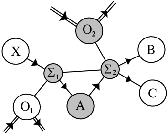
Figure 1: A typical quantum process. Arrows point from initial states to their tests and then to their outcomes, and give the local direction of time on the q-tick level. Shaded components belong to the active present.

A typical process is shown in figure $1.$ In this diagram, complex $O_{1}$ provides information which determines test $\Sigma_{1}$ of event $X$, with resolved outcome at event $A$. Subsequently, complex $O_{2}$ and test $\Sigma_{1}$ determine test $\Sigma_{2}$ of event $A,$ with an unresolved outcome at this particular stage. It happens to be a direct product state and hence can be represented by events $B$ and $C$.

The active present consists of tests $\Sigma_{1}$ and $\Sigma_{2}$, event $A$ and complex $O_{2}$, and therefore these are shaded. Event $X$ and complex $O_{1}$ belong to the absolute past, whilst events $B$ and $C$ belong to the future.

Such diagrams are dynamic, in that they depend on the stage in the history of the Universe being described.

2.2 Quantum automata

The concept of a cell is used in the theory of cellular automata [17] as a temporally enduring container which contains a time dependent variable. This variable is usually discrete, its value at any given discrete time being determined by the values of the variables in neighboring cells at earlier times. There are numerous references to cellular automata in the literature discussing discrete spacetime.

Such cellular automata are inadequate representations of the running of the Universe, because the events envisaged in this paper do not have any sort of identity which propagates into the future. The Universe is more accurately described as a quantum automaton. The main characteristic of such an automaton is that the discrete topological relations between events and tests in the future is uncertain. These relations depend on outcomes of tests which have not occurred at a given stage.

3 The Machine Observer

Once the notion of a conscious observer has been bypassed, the questions remain of how states are prepared and then how they are tested. It must be the case that on a fundamental level, the Universe runs as a vast quantum automaton. Its active present determines its own tests and then the random outcomes of these tests become involved in a new active present, which then determines the next set of tests. This leap-frog process proceeds ad infinitum on a vast scale of events. Each small part of classical reality is formed when any particular outcome is resolved (state reduction), which is the end of one q-tick and the start of the next one, locally.

The process of time is, therefore, directly related to state reduction and it proceeds irreversibly. It is non-integrable, in that there is no universal clock regulating the running of the Universe. A single q-tick could in principle last over the entire history of the Universe from the Big Bang to the present, or it could appear to last on a Planck scale. An analogy with the single celled organism amoeba is useful: an amoeba flows steadily towards its food, as advanced pseudopods reach out forwards whilst others retain their hold for a while on places where the organism had been. Eventually the whole organism moves forwards.

Q-ticks are not involved with Schrödinger time evolution; quite the contrary. Schrödinger evolution occurs in continuous time quantum mechanics precisely in the absence of a q-tick and represents the process of non-observation of a state of a system. From the perspective of this paper, the time in Schrödinger evolution is a marker of q-ticks involved with emergent observers, not the system being observed. The possibility of transforming to the Heisenberg picture supports this view, for in the Heisenberg picture states do not evolve whilst operators involved in tests do evolve.

At the end of a q-tick the following principle holds:

The weak quantum principle: The outcome of any test on an event state is an eigenstate of some Hermitian operator associated with that test.

This says something about the future and is a milder version of another principle saying something about the past and the future:

The strong quantum principle: Every event state is an eigenstate of some Hermitian operator representing a test. 

The difference between these principles is that the strong quantum principle rules out “Garden of Eden” states. These are states which could not be explained as the outcomes of past tests. Such a concept is encountered in the theory of cellular automata [17], and is relevant to the origin of the Universe, which is outside the scope of the present paper.

3.1 Null tests and unobserved phases

In real experiments, physicists can prepare states and then decide not to test them for arbitrary lengths of time, as measured by clocks associated with the physicists. A typical process is shown in figure $2a$. Here a complex of tests $\Sigma_{0}$ has a complex of outcomes $O_{0}$, which represents an emergent observer. This constructs a test $\sigma$ which prepares an outcome state $\psi,$ which serves as an initial state for a subsequent test $\Lambda$ with outcome $\phi$. The observer meanwhile runs on to $O_{1}$ and then to $O_{2},$ and only then constructs test $\Lambda.$

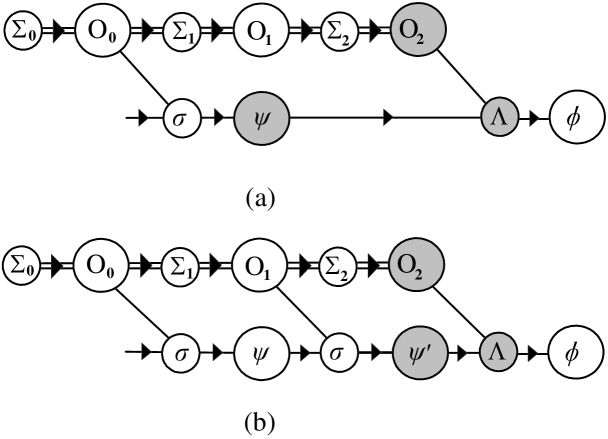
Figure 2: Two equivalent diagrams. In $2b$ a null test is included. The outcome $\psi^{\prime}$ is in the same ray as the initial state $\psi$ of the test.

In figure $2\left(b\right)$, a physically equivalent diagram suggests that $O_{1}$ has performed a null test $\sigma$ on $\psi$, which has had no physical effect. The outcome is $\psi^{\prime}$ which must be proportional to $\psi,$ because no real information can be passed back to the observer. A null test is physically equivalent to not doing a test on a state.

In this and other examples, the null test can be represented by the same operator $\hat{\sigma}$ which had as outcome  $|\psi\rangle,$ the initial state. The initial state is an eigenstate of $\hat{\sigma}$, according to quantum principles. The possible outcomes of the null test are also eigenstates of $\hat{\sigma}$ and these differ from the eigenstates of the original preparation test by at most random phases. Taking into account the probabilities of the possible outcomes, which are given by

$$P\left(\psi^{\prime}|\psi\right)\equiv|\langle\psi^{\prime}|\psi\rangle|^{2},$$ (5)

it is easy to see that the outcome $|\psi^{\prime}\rangle$ of the null test must be given

$$|\psi^{\prime}\rangle=e^{i\theta}|\psi\rangle,$$ (6)

because it occurs with probability one. All other eigenstates of the null test occur with probability zero.

In ($\ref{556})$, the phase $\theta$ is arbitrary. No physical information therefore can reside in this phase. This is consistent with the fact that the initial state $|\psi\rangle$ is itself fixed only up to some arbitrary phase.

Null tests are important because they must be involved in disentanglement in some way. This will be discussed in the section on the EPR paradox below.

Physical null tests can always be constructed in the laboratory by real physicists. These first prepare a state by choosing a given outcome of some test, which therefore serves as a filter. The equivalent of a null test is then made by passing such a prepared state through a physically equivalent filter. For example, an electron prepared in a spin-up state by being passed into the spin up channel of a Stern-Gerlach apparatus with quantization axis $+\mathbf{k}$ will automatically pass into the spin-up channel in a second Stern-Gerlach experiment with the same quantization axis, even if both channels are open in the second experiment.

In this example, note that what is required for the construction of a real null test is information about the preparation of the initial state. This information is carried into the future by the physicists as they themselves evolve in time, and then used to construct the second filter. In the framework discussed in this paper, the machine Universe will have available to it information about tests it carried out in the past, and about the outcomes of those tests. Therefore, in principle, the machine Universe does have all the information it requires to inform null tests on given states. Something like this must happen in EPR experiments.

3.2 Example

An example is now given of a system which constructs tests of itself which depend on its current state and other information from the past. In this toy model the active present always consists of a single event labelled by $E$ and indexed by an integer $n$. As the universe runs, the active event changes from $E_{n}$ to $E_{n+1}$ at the end of a q-tick, and so on. The event state $|\psi_{n}\rangle$ in each $E_{n}$ is some element of two dimensional spin space $\mathcal{H}_{2}$ with basis set $\left\{|\uparrow\rangle,|\downarrow\rangle\right\}.$

The model starts running at time $n=0$. Now in accordance with the strong quantum principle stated above, the event state $|\psi_{0}\rangle$ of the universe at that time must be an eigenstate of some operator $\hat{\Sigma}_{0}$, which represents the net effect of whatever happened in the past in this universe before that time, or the equivalent of the moment of the Big Bang. This operator is taken to have the form

$$\hat{\Sigma}_{0}\equiv\mathbf{\sigma}\cdot\mathbf{a,}$$ (7)

where the components of $\mathbf{\sigma}$ are the Pauli matrices and $\mathbf{a}$ is some unit three-vector. Such an operator has only two eigenstates, with eigenvalues $+1$ and $-1$ respectively. Hence the following eigenvalue equation must hold:

$$\hat{\Sigma}_{0}|\psi_{0}\rangle=\lambda_{0}|\psi_{0}\rangle,$$ (8)

where $\lambda_{0}=+1$ or else $\lambda_{0}=-1$.

It is here that classical information occurs. The eigenvalue $\lambda_{0}$ cannot be uncertain, even if it is unknown to any emergent observer (if such a phenomenon were possible in this model). This information is predicated on the nature of $\hat{\Sigma}_{0}$.

According to the machine principle, the state of the universe at time $t=n$ and other information from the past alone determine the test $\Sigma_{n+1}$ which will be applied to $E_{n}$ during the next q-tick. In the model, $\Sigma_{n+1}$ is represented by the Hermitian operator

$$\hat{\Sigma}_{n+1}\equiv\frac{{}_{1}}{{}^{2}}\left(1+\lambda_{n}\right)\hat{U}\hat{\Sigma}_{n}\hat{U}^{\dagger}+\frac{{}_{1}}{{}^{2}}\left(1-\lambda_{n}\right)\hat{V}\hat{\Sigma}_{n}\hat{V}^{\dagger},\;\;\;n=1,2,\ldots$$ (9)

where the operators $\hat{U}$ and $\hat{V}$ are elements of $SU\left(2\right)$. These operators are regarded here as generated by the laws of physics in this particular universe with no further explanation as to their origin. The diagram for the running of this toy universe is given in figure. $3$:

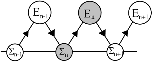
Figure 3: The running of the given toy universe.

The test $\Sigma_{n+1}$ represented by operator $\hat{\Sigma}_{n+1}$ requires information from the immediate past, not only about the state of the event $E_{n}$ but also about the test $\Sigma_{n}$ which led to it. Without all of this information the eigenvalue $\lambda_{n}$ is undetermined and so $\hat{\Sigma}_{n+1}$ cannot be constructed by the machine.

Assuming that information about $\lambda_{n}$ is available, then $\hat{\Sigma}_{n+1}$ can be constructed by the machine universe. The eigenvalues of this operator are always $\pm 1$, so that the future is uncertain before the next q-tick. At the end of that q-tick, however, the active present of the Universe shifts to event $E_{n+1}$, with $|\psi_{n}\rangle$ collapsing onto one of the two possible outcomes of the eigenvalue equation

$$\hat{\Sigma}_{n+1}|\psi_{n+1}\rangle=\lambda_{n+1}|\psi_{n+1}\rangle,$$ (10)

where $\lambda_{n+1}=\pm 1.\;$

In the model, the operators $\hat{U}$ and $\hat{V}$ may be assumed incommensurate, i.e., there exist no positive integers $p,q$ such that $\hat{U}^{p}=\hat{V}^{q}.\;$Then given $|\psi_{0}\rangle,$ $\lambda_{0}$ and $\hat{\Sigma}_{0}$ there are four distinct possible states of this universe at the end of the second q-tick, $n=2$. These are characterized by the four possible histories given in terms of the eigenvalues $\left(\lambda_{1},\lambda_{2}\right)$, vis;

$$\left(\lambda_{1},\lambda_{2}\right)=\left(+1,+1\right),\;\left(+1,-1\right),\;\left(-1,+1\right),\;\left(-1,-1\right).$$ (11)

Which one of these possibilities is taken is fundamentally a quantum process and cannot be predicted or forced. Starting from one state at time zero, the number $N_{n}$ of distinct possible branches of the universe is $2^{n}$ at time $n$, but only one of them will occur then.

In this model, the past is unique whereas the future is uncertain. There is only one state at any given time, so that the present is unique also. Because outcomes are quantum processes, however, the past cannot be uniquely retrodicted from information about the present.

In this model, time runs physically because classical information about the eigenvalue $\lambda_{n}$ has to be extracted at the end of each q-tick in order to determine the next test. An outcome has to occur for time to run, in other words.

3.3 The Einstein-Podolsky-Rosen paradox

The principles applied to elementary quantum processes can also be applied when emergent observers are involved. These are complexes of events and tests which to all intents and purposes can be treated diagrammatically as single events. Because the emphasis here is on tests as much as on the states being tested, the approach provides some insight into how conventional measurements are made on emergent scales.

The Einstein-Podolsky-Rosen thought experiment [25] deals with entangled states. When certain observations are made on such states, non-classical consequences can follow which strongly support the view that quantum processes are non-local. This has been reinforced by experiments on Bell inequalities and supports the approach taken in this paper, which does not assume space exists at a fundamental level.

The version of the EPR scenario discussed here is the spin half bound state example favoured by Bohm. Consider the creation of a neutral pion $\pi^{0}$ at time $t=0$ in some inertial frame $\mathcal{F}$ and its subsequent decay into an electron-positron pair. The total spin $s$ of the state remains zero during the decay, so its spin structure may be considered to be that of two spin half particles in the entangled form

$$|\pi\rangle\equiv\frac{{}_{1}}{{}^{\sqrt{2}}}\left\{|+\mathbf{k}\rangle_{e}\otimes|-\mathbf{k}\rangle_{p}-|-\mathbf{k}\rangle_{e}\otimes|+\mathbf{k}\rangle_{p}\right\}$$ (12)

relative to the standard tensor product space basis, where $\mathbf{k}$ is a unit vector along the $z$-direction quantization axis and the subscripts $e$ and $p$ refer to the electron and positron respectively [15].

If an observer $O$ subsequently decided to test the spin of the system, such a test would be represented by the operator

$$\hat{\Sigma}\left(\mathbf{a}\right)\equiv\left(\mathbf{\sigma}_{e}\mathbf{\cdot a}\right)\otimes\hat{I}_{p}+\hat{I}_{e}\otimes\left(\mathbf{\sigma}_{p}\mathbf{\cdot a}\right),$$ (13)

where $\mathbf{\sigma}\equiv\left(\sigma^{1},\sigma^{2},\sigma^{3}\right)$ are the Pauli matrices, $\mathbf{a}$ is a unit vector pointing in some direction chosen by $O$ after the state has been prepared and $\hat{I}_{e}$ and $\hat{I}_{p}$ are identity operators in their respective component spaces of the tensor product space. Factors of $\frac{{}_{1}}{{}^{2}}\hbar$ will be ignored here. This process is represented by figure $4$.

In this diagram, the initial state-event of the pion is represented by the circle labelled $\pi$. The line with an arrow from the left of this event comes from some test of which the pion was a particular outcome and which is not shown. The circle labelled $O$ represents an emergent observer involved with the test of the pion labelled $\Sigma\left(\mathbf{a}\right)$. The double line with an arrow going into $O$ implies that $O$ is itself the result of a large, possibly vast number of outcomes of tests in the immediate past, and these are not shown. The observer $O$ is a complex of elementary events, that is, $O$ is an emergent process, and for convenience has been shown as one circle. It is a feature of the present formulation that no part of $O$ is an unresolved outcome of a test; state resolution (reduction) has definitely occurred in each component event making up $O$. The observer may also consist of various tests, which are not quantum objects themselves. Therefore overall, the observer is semi-classical.

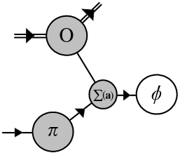
Figure 4: A single local test $\Sigma\left(\mathbf{a}\right)$ on a neutral pion state $\pi$, with outcome $\phi.$ O represents a complex of events making up the emergent observer.

The line without an arrow connecting $O$ with the test $\Sigma\left(\mathbf{a}\right)$ indicates that a vast amount of information from $O$ may be involved in setting up this test, whereas a single line with an arrow from $\pi$ to $\Sigma\left(\mathbf{a}\right)$ represents a test of that state. The outcome of the test $\Sigma\left(\mathbf{a}\right)$ is shown as a future event $\phi$, that is, one not yet resolved, and is therefore an unshaded circle according to the notation.

It is a particular property of the state $\left(\ref{389}\right)$ that it may be written in the alternative form

$$|\pi\rangle=\frac{{}_{1}}{{}^{\sqrt{2}}}\left\{|+\mathbf{a}\rangle_{e}\otimes|-\mathbf{a\rangle}_{p}-|-\mathbf{a}\rangle_{e}\otimes|+\mathbf{a}\rangle_{p}\right\},$$ (14)

where the component states such as $|+\mathbf{a}\rangle_{e}$ are eigenstates of the component operators $\mathbf{\hat{\sigma}}_{e}\mathbf{\cdot a}$ in $\hat{\Sigma}\left(\mathbf{a}\right)$ respectively. It is readily seen that state $\left(\ref{299}\right)$ is an eigenstate of $\hat{\Sigma}\left(\mathbf{a}\right)$ with eigenvalue zero, confirming that the original state is spinless.

The $EPR$ paradox arises when two different and widely separated emergent observers $O_{1}$ and $O_{2}$ each decide to perform their own experiment on just one of the constituent particle spins. This is possible here because $O_{1}$ could filter out the positron because of its positive electric charge and test only for the electron spin (say), and similarly $O_{2}$ could filter out the electron and test only for positron spin. It is at this point that free will appears to enter into the picture, which is the source of the problem.

Observers $O_{1}$ and $O_{2}$ will consist of enormous patterns of events and tests which on emergent scales have consciousness and the belief structures that they are at rest and widely separated in the same inertial frame with their conventional clocks synchronized. Suppose this is the case, and now suppose further that on one side of the Universe, observer $O_{1}$ decides at emergent (co-ordinate) time $t=T>0$ to perform a Stern-Gerlach experiment on the electron only whereas on the other side of the Universe observer $O_{2}$ decides at the “same time” $t=T$ to perform a Stern-Gerlach experiment on the positron only.

Observer $O_{1}$ therefore performs a test $\Sigma_{1}$ which they believe is described by the operator

$$\hat{\Sigma}_{1}\equiv\mathbf{\hat{\sigma}}_{e}\cdot\mathbf{b,}$$ (15)

acting on the electron state space only, whereas observer $O_{2}$ performs a test $\Sigma_{2}$ which they believe is described by the operator $\hat{\Sigma}_{2}\equiv\mathbf{\hat{\sigma}}_{p}\mathbf{\cdot c}$ acting on the positron state space only. Here $\mathbf{b}$ and $\mathbf{c}$ are unit vectors chosen by observers $O_{1}$ and $O_{2}$ respectively, with apparently full freedom to choose any directions for these vectors.

This freedom is the source of the problem. Suppose $O_{1}$ chooses axis $\mathbf{b}$. There are only two possible outcomes of the test $\Sigma_{1}.\;$Either the electron has spin $|+\mathbf{b}\rangle_{e}$ and therefore the positron must be in state $|-\mathbf{b\rangle}_{p},$ or else the electron has spin $|-\mathbf{b}\rangle_{e}$ and therefore the positron must be in state $|+\mathbf{b\rangle}_{p}$. This is because total angular momentum is conserved.

This means that regardless of where in the Universe observer $O_{2}$ is, their choice of test $\Sigma_{2}$ will have outcomes apparently dictated by the outcome of test $\Sigma_{1}.\;$This leads to certain predictions involving Bell inequalities and ultimately to a conflict with Einstein locality [15], and is the source of endless debate in quantum mechanics.

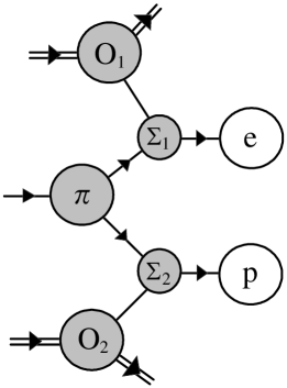
Figure 5: A diagram such as this is forbidden because $\pi$ is entangled.

In a diagrammatic representation of these observations, the classical and erroneous EPR picture of what is going on would represented by figure $5$. This suggests that separate parts of the entangled system are being tested separately, and this is the source of the EPR problem. According to quantum principles, a null test yields no new information and therefore leaves a state essentially unchanged, whereas the extraction of new information about a state must alter it. Therefore, only one non-null test of a state is possible. The only circumstance where the equivalent of two independent tests on the same event state is possible is if that state were a direct product, and under those circumstances, one test would have to involve one factor of the product states and the other test would have to involve another factor. This is not possible when the initial state is entangled, as in the present case. There is therefore a veto on diagrams such as figure $5$ when $\pi$ is entangled.

This leads to the following principle:

The entanglement principle: An entangled event state can be tested by only one test, whereas each factor state of a direct product event state can be tested separately.

This principle permits a discussion of the Universe in terms of observers and systems, because the state of the Universe appears not to be completely entangled.

The entangled nature of the initial pion state requires an alternative diagrammatic description of the above experiment. Given that continuous time and space do not exist per se and that quantum processes occur over single q-ticks, the running of the Universe must take one of two topologically distinct patterns of tests, shown in figures $6a$ and $6b$ respectively:

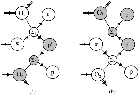
Figure 6: The two alternative and exclusive topologically distinct combinations of tests which measure individual spins in an entangled state at widely separated places in the Universe. A combined test takes two q-ticks.

The interpretation of figure $6a$ is the following. A $\pi^{0}$ state is created at the event labelled $\pi$. This state is not only an eigenstate of the operator $\left(\ref{888}\right)$ but also of the angular momentum multiplet operator

$$\hat{S}^{2}\equiv\sum_{i=1}^{3}\left(\hat{\sigma}_{e}^{i}\otimes\hat{I}_{p}+\hat{I}_{e}\otimes\hat{\sigma}_{p}^{i}\right)\left(\hat{\sigma}_{e}^{i}\otimes\hat{I}_{p}+\hat{I}_{e}\otimes\hat{\sigma}_{p}^{i}\right),$$ (16)

with eigenvalue zero. Although the creation of the pion is the outcome of a single test not shown in figure $6$, the operator $\left(\ref{888}\right)$ on its own is insufficient to pin down the state of the pion and represent that test fully.

When observer labelled $O_{1}$ decides to test for the electron spin with test given by $\left(\ref{896}\right)$, $O_{1}$ is apparently not testing anything about the positron. So it could be reasonably be asked, what forces the positron into an opposite spin state to the electron? The answer is given by the machine principle, which says that the automatic running of the machine universe itself ensures the positron comes out from $\Sigma_{1}$ in such a way as to ensure total spin conservation. In other words, some additional component to the test $\Sigma_{1}$ must be involved.

The real test $\Sigma_{1}$ therefore must require any outcome to be a simultaneous eigenstate of the two operators

$$\hat{\Sigma}_{1}^{(1)} = \left(\mathbf{\hat{\sigma}}_{e}\cdot\mathbf{b}\right)\otimes\hat{I}_{p}$$ (17)

$$\hat{\Sigma}_{1}^{\left(2\right)} = \left(\mathbf{\hat{\sigma}}_{e}\mathbf{\cdot b}\right)\otimes\hat{I}_{p}+\hat{I}_{e}\otimes\left(\mathbf{\hat{\sigma}}_{p}\mathbf{\cdot b}\right).$$ (18)

A convenient basis $\mathcal{B}$ for solutions to this problem is given by the direct products

$$\mathcal{B}=\left\{|+\mathbf{b\rangle}_{e}\mathbf{\otimes|+b\rangle}_{p}\mathbf{,\,|+b\rangle}_{e}\mathbf{\otimes|-b\rangle}_{p}\mathbf{,\,|-b\rangle}_{e}\mathbf{\otimes|+b\rangle}_{p}\mathbf{,\,|-b\rangle}_{e}\mathbf{\otimes-b\rangle}_{p}\right\},$$ (19)

where

$$\mathbf{\hat{\sigma}}_{e}\cdot\mathbf{b}|+\mathbf{b\rangle}_{e}=+|+\mathbf{b\rangle}_{e},$$ (20)

and so on. Eigenstates of the first operator $\hat{\Sigma}_{1}^{(1)}$ are of the form

$$|+\rangle = \alpha|+\mathbf{b\rangle}_{e}\mathbf{\otimes|+b\rangle}_{p}+\beta\mathbf{|+b\rangle}_{e}\mathbf{\otimes|-b\rangle}_{p},$$

$$|-\rangle = \gamma\mathbf{\,|-b\rangle}_{e}\mathbf{\otimes|+b\rangle}_{p}+\delta\mathbf{\,|-b\rangle}_{e}\mathbf{\otimes|-b\rangle}_{p},$$ (21)

with eigenvalues $\lambda^{\left(+\right)}=+1$ and $\lambda^{\left(-\right)}=-1$ respectively. The information about which eigenvalue occurs is transmitted to the emergent observer $O_{1}$ and is interpreted as an electron in one of the two possible spin states $|+\mathbf{b\rangle}_{e}$ or $|-\mathbf{b\rangle}_{e}\mathbf{.}$

The coefficients $\alpha,\,\beta,\,\gamma$ and $\delta$ in $\left(\ref{356}\right)$ are not arbitrary and are determined by the requirement that the states $|+\rangle$ and $|-\rangle$ are also eigenstates of $\hat{\Sigma}_{1}^{\left(2\right)}$ and the crucial requirement that no new information is extracted from that sub-test by either $O_{1}$ or the machine Universe. This means that $|+\rangle$ and $|-\rangle$ must each have eigenvalue $zero$ relative to $\hat{\Sigma}_{1}^{\left(2\right)}.$ In effect, $\hat{\Sigma}_{1}^{\left(2\right)}$ represents the action of a null test on the components of the entangled state. This requirement fixes the coefficients in $\left(\ref{356}\right)$ giving

$$|+\rangle = \mathbf{|+b\rangle}_{e}\mathbf{\otimes|-b\rangle}_{p},$$

$$|-\rangle = \mathbf{\,|-b\rangle}_{e}\mathbf{\otimes|+b\rangle}_{p},$$ (22)

ignoring arbitrary overall phases. These occur with probability one half each. Note that the test $\Sigma_{1}$ has an outcome which is not an eigenstate of the multiplet operator $\left(\ref{999}\right).$

Because observer $O_{1}$ has acquired information from test $\Sigma_{1}$, a single q-tick has definitely occurred then. However, $O_{1}$ will almost certainly believe that a much greater time has elapsed than just one q-tick, because according to them, their local time is measured by their own internal processes, which take place over vast numbers of q-ticks. These are not shown but implied by the double lines entering and leaving the circle representing $O_{1}.$

Because the outcome of test $\Sigma_{1}$ is a product state, it can be shown as two events, labelled $e$ and $p^{\prime}$ in figure $6a$. The event state $|p^{\prime}\rangle\;$is one of the positron states $\mathbf{|+b\rangle}_{p},\mathbf{|-b\rangle}_{p}$ in $\left(\ref{478}\right)\,$and this now feeds into test $\Sigma_{2},$ which has been set up by observer $O_{2}$ and who believes themselves to be on the other side of the universe to $O_{1}$. This test will have as outcome event $p$, which occurs on the second q-tick after the creation of the initial state $\pi$.

Even though $O_{1}$ and $O_{2}$ may believe that they are separated by vast distances, the quantum processes given in figure $6a$ do not have any cognisance of this. These distance estimates are particular emergent attributes of the Universe calculated by the emergent observers via relatively straightforward counting processes, in line with Riemann’s idea that distance is a numerical count of fundamental units [1].

The entire process could follow an alternative path, given by figure $6b.$ The two diagrams, figures $6a$ and $6b$ suggest that such experiments cannot be carried out absolutely simultaneously in terms of q-ticks at different parts of the universe. This is nothing to do with relativity at all. One of the tests must always be one q-tick later than the other. This is a topological relationship between outcomes of tests, and in that sense involves the structure of spacetime. Co-ordinate or laboratory times estimated by the two emergent observers relate to emergent descriptions of the Universe. They may appear to be simultaneous to all intents and purposes, because they count time in terms of vast numbers of q-ticks, most of which may be thought of as occurring on Planck scales.

It is conceivable that one day technology might be found to establish whether these topological structures are relevant in such processes, but it likely that there might be no way in principle of determining whether process $6a$ or $6b$ had occurred in an actual run of the experiment.

It is possible that the choice of which of these processes is actually taken by the running of the universe may itself be thought as the outcome of some higher order quantum test. This would perhaps be equivalent to “second quantization”, i.e., a quantum test whose outcomes are themselves different tests, rather than states. Since these tests involve different topologies, as in figures $6a$ and $6b$, there is here a scenario for an approach to quantum spacetime topology, otherwise known as quantum gravity. That is outside the scope of this paper and is a matter reserved for the future.

Discussions of Bell inequalities will remain unchanged in the approach discussed here, because all the standard correlations of quantum mechanics will be reproduced. What the diagrammatic approach taken here has done is to emphasize why these correlations should occur. These inequalities deal with expectation values, so they refer to emergent processes. These can be dealt with straightforwardly here because the machine principle does not excluded the emergent level. The use of emergent observers in the discussion validates a discussion of probabilities, because these observers can make the choice of repeating experiments such as the one discussed above.

4 Particle decays and scattering

These ideas can be applied to particle decays and scattering processes. Consider the former. The question of particle decay lifetime involves a balance of heuristics and formal theory, because the interpretation of what is going on lies on the borderline between the classical and the quantum. According to the notion of a q-tick, an elementary particle decay involves one q-tick, whereas conventional time is measured on emergent scales and normally involves vast numbers of q-ticks. The question arises as to what the physical meaning of decay lifetime is.

The answer comes from the Heisenberg picture in quantum mechanics. In this picture, a state remains frozen in time and all the time dependence is transferred onto the observables, the physical operators of the theory. This is in line with the approach taken in this paper. Observables represent tests, and their time dependence is a manifestation of time as it runs in the Universe external to the state being observed.

It is useful to review briefly the usual approach to particle decays from both the Schrödinger and Heisenberg pictures.

4.1 The Schrödinger picture

In this picture an initial state $|\psi\rangle$ is prepared at time $t_{i}\;$and allowed to evolve quantum mechanically until a final time $t_{f}>t_{i}$, at which time the evolved state  $|\psi,t_{f}\rangle$ is tested to see if it has decayed. Suppose the decayed state looked for is $|\phi\rangle$. This state may be assumed an eigenstate of some operator $\hat{\Lambda}$, vis,

$$\hat{\Lambda}|\phi\rangle=\lambda|\phi\rangle.$$ (23)

Then the probability $P\left(\phi|\psi\right)$ that the outcome of the test is $|\phi\rangle$ is just

$$P\left(\phi|\psi\right)=|\langle\phi|\hat{U}\left(t_{f},t_{i}\right)|\psi\rangle|^{2},$$ (24)

where $\hat{U}\left(t_{f},\,t_{i}\right)$ is the time evolution operator. In this picture, the initial state is assumed to change in time according to the rule

$$|\psi\rangle\rightarrow|\psi,t_{f}\rangle\equiv\hat{U}\left(t_{f},t_{i}\right)|\psi\rangle.$$ (25)

The probability $P\left(\phi|\psi\right)$ is then transformed via a conventional heuristic formalism into the decay lifetime associated with the transition $|\psi\rangle\rightarrow|\phi\rangle$

A particularly subtle point is this. In this scenario, there is a vast amount of information assumed about the time evolution and the measurement process, which is understood by experimentalists and theorists intuitively, but which is not mathematically incorporated into the formalism per se. The physical interpretation of the probability $P\left(\phi|\psi\right)$ is that it is the probability that a test made at time $t_{f}$ for the occurrence of state $|\phi\rangle$ had a positive outcome, given that no attempt had been made to look at the initial state up to that time and extract information about it. This is classical information about what the observers have done or not done during the time interval $\left[t_{i},t_{f}\right]$.

In other words, even in the Schrödinger picture, which gives the impression that the only time evolution occurring lies with the state, the behaviour of the observer in time is just as crucial. Knowing that a test has not yet been done on a system is a piece of information which is just as important in a quantum measurement as knowing that a test has been done.

4.2 The Heisenberg picture

This picture is fully consistent with the notion of a q-tick. In this picture, all time dependence is transferred explicitly onto observers and tests. Once prepared, an initial state is frozen until it is tested. This is much more natural a picture in terms of quantum principles than the Schrödinger picture. It could be argued that latter is somewhat inconsistent, because a prepared state which is not being tested is effectively decoupled from the Universe, so how could any sort of notion of time be associated with it? How does an isolated state have any information about co-ordinate time, which is measured by on observer decoupled from that state?

In the Heisenberg picture, time runs for observers, and when they construct tests this time dependence is encoded in those tests. According to this picture, the decay experiment discussed above is described as follows. First the observer constructs the state $|\psi\rangle$ at time $t_{i}$. This state is left completely alone until time $t_{f}>t_{i},$ at which time the observer tests for the probability that the initial state has component $|\phi,t_{f}\rangle.$ This state is an eigenstate of the operator $\hat{\Lambda}\left(t_{f}\right)\equiv\hat{U}^{\dagger}\left(t_{f},\,t_{i}\right)\hat{\Lambda}\hat{U}\left(t_{f},t_{i}\right)$ with the same eigenvalue $\lambda\;$as in $\left(\ref{666}\right)$. It is the eigenvalue which identifies to the observer the state being measured. A solution is given by

$$|\phi,t_{f}\rangle=\hat{U}^{\dagger}\left(t_{f},t_{i}\right)|\phi\rangle,$$ (26)

and so the probability of the transition occurring is exactly the same as for the Schrödinger picture, equation $\left(\ref{199}\right).$

4.3 The q-tick picture

From the point of view of the picture given in this paper, a decay experiment can be represented by a diagram such as figure $7.$

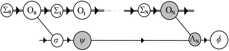
Figure 7: The q-tick picture in a decay or scattering process as seen on the fundamental and emergent levels.

Here the observer runs as a quantum automaton from its initial configuration $O_{0}$ to some final configuration $O_{N}$, via a vast number of q-tick processes, characterized by some integer $N$, whereas the decays process takes precisely one q-tick on the fundamental level. Almost certainly, $N$ would not be precise, not because of any uncertainty in the topology of events, but because time on a fundamental level in not integrable. However, on emergent scales, estimates of the average number of q-tick processes should be meaningful and it is these estimates which translate into estimates by emergent observers into their laboratory time. There is no fundamental scale per se in this framework, but if typical q-ticks associated with emergent observers were counted to be more-or-less equivalent to Planck units, then the decay of a $\pi^{0}$ takes about $10^{27}$ of these observer q-ticks, i.e., $N\sim 10^{27}.$

The test performed by $O_{N}$ will be represented by some operator $\hat{\Lambda}_{N}$, which carries information supplied by $O_{N}$. If $O_{N}$ forms part of a sequence of observer events $O_{1},O_{2},\ldots$ which is homogeneous in the sense that no radical changes occur in the laboratory environment associated with each element of this sequence, than the simplest ansatz which could be applied would be to take

$$\hat{\Lambda}_{N}=\hat{U}^{\dagger N}\hat{\Lambda}U^{N},$$ (27)

where $\hat{U}$ is an elementary unitary time-step operator of the form discussed in [26]. The picture which emerges corresponds precisely to the Heisenberg picture in the continuous time formulation.

5 Discussion

A number of fundamental issues remain to be discussed in this framework, and these will be considered elsewhere. They include irreversibility, the early machine Universe, Schrödinger’s cat, the quantum Zeno effect, superselection rules and unbounded operators such as position and momentum. It is likely that the emphasis placed here on tests as much as on their outcomes should have a lot to say about some of these issues. For example, if the strong quantum principle holds, then the issue about the origin of the Universe really concerns the test which produced the initial state, and not so much that initial state. Likewise, the Schrödinger’s cat issue really concerns the physical existence or not of a test which could produce a state which was a linear combination of a living cat and a dead cat. If such a test cannot be constructed physically, then the question of such a linear superposition does not arise. The same remark holds for superselection rules forbidding linear combinations of states with different electric charges.

On the physical meaning of time, the position taken in this paper is that it is a real phenomenon and that the Universe runs. This contrasts with some emergent theories such as general relativity, where general covariance leads to a view which is unsettling and counter intuitive. Time appears to freeze out in such theories when quantisation is attempted. It should be noted that such a result can be found in any Lagrangian model using Dirac’s reparametrisation method [27] involving constraint mechanics, but that does not eliminate the physical reality of time in such models.

Since time as discussed in this paper is not directly related to an integrable parameter except on emergent scales, an obvious conclusion is that the Euclidean formulation of time, wherein real time is rotated into the imaginary axis, is meaningful only in an emergent context. Theories which use it exclusively cannot be truly fundamental. Lattice gauge theories formulated on four dimensional Euclidean lattices are reasonable because this approach is regarded as an approximation method. Cosmological theories which are formulated exclusively in Euclidean spacetimes must be regarded as unphysical from the point of view of this paper, as are attempts to regularize quantum gravity by appealing to imaginary time.

Finally, because in the framework discussed here time is the acquisition of quantum information, there is no scope here for closed timelike curves, and any theory which permits them must be emergent and therefore not fundamental.

Acknowledgments:

I am indebted to Drs Rosolino Buccheri and Vito Di Gesù and the other organizers and participants of the First International Interdisciplinary Workshop: Studies on the Structure of Time: from Physics to Psycho(Patho)logy, held in Palermo in November $1999$, for giving me the stimulation and motivation to carry out this work. I am grateful to Keith Norton and Jon Eakins for all their views, comments and discussions with me on the nature of time.

References

- [1] D. Meyer, L. Bombelli, J. Lee and R. Sorkin, Space-Time as a Causal Set, Phys. Rev. Lett., 59(5): 521–524, 1987.
- [2] Fotini Markopoulou, Quantum causal histories, Class. Quant. Grav., 17: 2059–2072, 2000.
- [3] Scott Hitchcock, Quantum clocks and the origin of time in complex systems, gr-qc/9902046, pages 1–18, 1999.
- [4] Manfred Requardt, (Quantum) spacetime as a statistical geometry of lumps in random networks, Class. Quant. Grav, 17:2029–2057, 2000.
- [5] P. A. Zizzi, The early universe as a quantum growing network, gr-qc/0103002, pages 1–16, 2001.
- [6] Lawrence Bragg, quote attributed to Bragg in ”Dynamical Solution to the Quantum Measurement Problem, Causality, and the Paradoxes of the Quantum Century”, by V.P. Belavkin, Open Sys. and Information Dyn. 7: 101-129, 2000.
- [7] G J Whitrow, The Natural Philosophy of Time, Clarendon Press, Oxford, 2nd Edition, 1980.
- [8] Roland Omnès, The Interpretation of Quantum Mechanics, Princeton University Press, Princeton, New Jersey, 1994.
- [9] D.P. Ridout and R.D. Sorkin, A Classical Sequential Growth Dynamics for Causal Sets, gr-qc/9904062, pages 1–28, 1999.
- [10] Manfred Requardt, Space-time as an orderparameter manifold in random networks and the emergence of physical points, gr-qc/99023031, pages 1–40, 1999.
- [11] Peter Halligan and David Oakley, Greatest myth of all, New Scientist, 18 November, pages 34–39, 2000.
- [12] S. Hagan, S. R. Hameroff, J. A. Tuszyǹski, Quantum Computation in Brain Microtubules? Decoherence and Biological Feasibility, quant-ph/0005025, pages 1-10, 2000
- [13] Roger Penrose, Shadows of the Mind, Oxford University press, 1994.
- [14] John C. Collins, On the compatibility between Physics and intelligent organisms, http://xxx.lanl.gov/physics/0102024, 2001.
- [15] Asher Peres, Quantum Theory: Concepts and Methods, Kluwer Academic Publishers, 1993.
- [16] E P Wigner, Remarks on the mind-body question, Symmetries and Reflections, pages 171–184, 1967, reprinted in Quantum Theory and Measurement, edited by J A Wheeler and W H Zurek,Princeton University Press, 1983.
- [17] Stephen Wolfram, Theory and Applications of Cellular Automata, World Scientific, 1986.
- [18] C. J. Isham, Lectures on Quantum Theory, Imperial College Press, 1995.
- [19] D. Deutsch, The structure of the multiverse, quant-ph/0104033, pages 1–21, 2001.
- [20] Scott Hitchcock, Feynman clocks, causal networks, and the origin of hierarchical ’arrows of time’ in complex systems. part i. ’conjectures’, gr-qc/0005074, pages 1–50, 2000.
- [21] Bryce S. DeWitt and Neill Graham, The Many-Worlds Interpretation of Quantum Mechanics, Princeton University Press, 1973.
- [22] David Deutsch, The Fabric of Reality, The Penguin Press, 1997.
- [23] Jaroszkiewicz G and Norton K, Principles of discrete time mechanics: II. Classical field theory, J. Phys. A: Math. Gen., 30(7): 3145–3163, May 1997.
- [24] George Jaroszkiewicz, Discrete spacetime: classical causality, prediction, retrodiction and the mathematical arrow of time, in V. Di Gesu, R. Buccheri and M. Saniga, editors, First International Interdisciplinary Workshop: Studies on the Structure of Time: from Physics to Psycho(Patho)Logy, 23-24 November 1999, CNR-Area della Ricerca di Palermo, Sicily, Kluwer Academic (New York), and in gr-qc/0004026.
- [25] B. Podolsky A. Einstein and N. Rosen, Can quantum mechanical description of reality be considered complete? Phys. Rev., 47: 777, 1935.
- [26] Jaroszkiewicz G and Norton K, Principles of discrete time mechanics: I. Particle systems, J. Phys. A: Math. Gen., 9(7): 3115–3144, May 1997.
- [27] Dirac P A M, Lectures on Quantum Mechanics, Yeshiva University (New York), Belfer Graduate School of Science Monograph Series, no 2, 1964.