Effect of noise on geometric logic gates for quantum computation

Abstract

We introduce the non-adiabatic, or Aharonov-Anandan, geometric phase as a tool for quantum computation and show how that phase on one qubit can be monitored by a second qubit without any dynamical contribution. We also discuss how that geometric phase could be implemented with superconducting charge qubits. While the non-adiabatic geometric phase may circumvent many of the drawbacks related to the adiabatic (Berry) version of geometric gates, we show that the effect of fluctuations of the control parameters on non-adiabatic phase gates is more severe than for the standard dynamic gates. Similarly, fluctuations also affect to a greater extent quantum gates that use the Berry phase instead of the dynamic phase.

I Introduction

To be useful, quantum computers will require long coherence time and low error rate. To attain this goal, good design and careful choice of the qubit’s operation point are crucial devoret:2002 . It is however believed that this will not be enough and that some kind of ‘software’ protection will be necessary. To achieve this, different strategies have been suggested: quantum error correction steane:99 , decoherence-free subspaces zanardi:97 ; lidar:98 and bang-bang control viola:98 .

Another approach to minimize the effect of imperfections on the controlled evolution of qubits is to use geometric phases and, in particular, the adiabatic geometric phase (or Berry’s phase) berry:84 . Contrary to the dynamic phase, Berry’s phase does not depend on time but is related to the area enclosed by the system’s parameters over a cyclic evolution in parameter space. It is therefore purely geometric in nature. As a result, it does not depend on the details of the motion along the path in parameter space: as long as the area is left unchanged the phase is left unchanged by imperfections on the path. This tolerance to area preserving imperfections has suggested to some authors that Berry’s phase could be a useful tool for intrinsically fault-tolerant quantum computation. For example, from the above argument, one is led to think that Berry’s phase gates will not be very sensitive to random noise along the path jones:2000 . Proposals for the observation and use of this phase for quantum computation have been given for different physical systems jones:2000 ; ekert:2000 ; falci:2000 . Application of the non-abelian geometric phase wilczek:84 to quantum computation was also the subject of several publications zanardi:99 ; duan:2001 ; choi:2001 ; faoro:2002 .

In this paper, we consider another type of geometric phase as a tool for quantum computation: the non-adiabatic, or Aharonov-Anandan (AA), geometric phase aharonov:87 . As Berry’s phase, the AA phase is purely geometric. It is related to the area enclosed by the state vector in projective space (see below) during a cyclic evolution. One would therefore believe that quantum gates based on this geometric phase also have some built-in tolerance to noise about the path. The use of this gate as a tool for intrinsically fault-tolerant quantum computation was also recently suggested in Ref. xiangbin:2001 .

In this paper we point out that, when compared to Berry’s phase, the AA phase seems to have many advantages for quantum computation. We also discuss quite generally how to monitor this global phase on one qubit using a second qubit. Implementation of the AA phase in a symmetric superconducting charge qubit makhlin:2001 is also discussed. Implementation in other quantum computer architectures is a simple generalization. The main point of this paper however is to show that the above arguments concerning tolerance to noise do not hold. Logical gates based on this phase are in fact more affected by random noise in the control parameters than equivalent dynamic gates. By studying the effect of random noise on the qubit’s control parameters, we are able to obtain a bound on the value of the phase beyond which the AA phase gate would be advantageous over its dynamical equivalent. In this way, we show that the AA phase is never useful in practice. This result is confirmed numerically for different noise symmetries. Moreover, using the same analytical and numerical approaches, we point out that quantum gates based on Berry’s phase are also more affected by fluctuations than their dynamical counterparts.

II Adiabatic vs non-adiabatic geometric phase gates

Let us begin by recalling the main ideas related to Berry’s phase and see what are its drawbacks for quantum computation applications. Consider a system whose Hamiltonian $H(t)$ is controlled by a set of external parameters $\mathbf{R}\mathit{(t)}$. Upon varying $\mathbf{R}\mathit{(t)}$ adiabatically, if the system is initially in an eigenstate of $H$ it will remain in an eigenstate of the instantaneous Hamiltonian. Moreover, if $H$ is non-degenerate on a closed loop $C$ in parameter space such that $\mathbf{R}\mathrm{(0)}=\mathbf{R}\mathit{(\tau)}$, the final state will differ only by a phase factor from the initial state. Berry has shown that this phase factor has both a dynamic and a geometric contribution, the later depending solely on the loop $C$ in parameter space berry:84 . If the initial state is a superposition of eigenstates $|\psi_{n}\rangle$ of the Hamiltonian, each of the eigenstates in the superposition will acquire a Berry phase $|\psi_{n}(\tau)\rangle=U(\tau)|\psi_{n}(0)\rangle=e^{i\phi_{n}}|\psi_{n}(0)\rangle$ for some real, eigenstate-dependent, phase $\phi_{n}$ anandan:87b . These phases will generally have both dynamic and geometric contributions. This is not a cyclic evolution of the state vector but this does not lead to any ambiguities since Berry’s phase is defined over parameter space.

It follows from the above that the application of adiabatic geometric phases to quantum computation has several drawbacks. First, quantum computers will very likely have a short coherence time. To take full advantage of this short time, the logic operations should be realized as fast as possible. The adiabaticity constraint means that Berry’s phase gates will be slow, thereby reducing the effective quality factor of the quantum computer.

Another drawback of the adiabatic phase gate is that during the adiabatic evolution, both geometric and dynamic phases are acquired. The later is not tolerant to area preserving noise and must be removed. This could be done using spin-echo like refocusing schemes which require going over the adiabatic evolution twice jones:2000 ; ekert:2000 ; falci:2000 . However, this further increases the time required to realize a single phase gate and imperfect operation will cause the dynamic phase not to cancel completely, thereby introducing errors.

A third difficulty is that adiabatic geometric phases are only possible if non-trivial loops are available in the space of parameters controlling the qubit’s evolution. In other words, the single-qubit Hamiltonian must be of the form

$$H=\frac{1}{2}B_{x}(t)\,\sigma_{x}+\frac{1}{2}B_{y}(t)\,\sigma_{y}+\frac{1}{2}B_{z}(t)\,\sigma_{z},$$ (1)

where control over all three (effective) fields $B_{i}(t)$ is possible. Such control is not possible in most of the current proposals for solid-state quantum computer architectures. Control over only two fields, say $B_{x}$ and $B_{z}$, is usually the norm. In this case, all loops in parameter space are limited to the $x$–$z$ plane and the (relative) Berry phase is limited to integer multiples of $2\pi$, of no use for computation. Control over fields in all three directions is possible in NMR where Berry phase gates have been implemented experimentally jones:2000 . More recently, Falci et al. falci:2000 have extended the original superconducting charge qubit proposal makhlin:2001 from a symmetric to an asymmetric design to allow a non-zero $B_{y}$ and therefore non-trivial closed paths in parameter space.

This need for external control of many terms in the single-qubit Hamiltonian means additional constraints, experimental difficulties and sources of noise and decoherence. This is clearly contrary to the efforts now invested in reducing quantum computer design complexity using the approach of encoded universality bacon:2001 .

As we shall see, all of the above issues, namely slow evolution, need for refocusing and control over many effective fields, seem to be resolved when one considers the non-adiabatic generalization of Berry’s phase: the Aharonov-Anandan (AA) phase.

The latter is introduced by restricting oneself, for a given $H(t)$, to initial states which satisfy

$$|\psi(\tau)\rangle=U(\tau)|\psi(0)\rangle=e^{i\phi}|\psi(0)\rangle.$$ (2)

For non-adiabatic evolutions, these so-called cyclic initial states moore:91 are generally not eigenstates of the system’s Hamiltonian but of the evolution operator. Aharonov and Anandan aharonov:87 have shown that the total phase $\phi$ acquired by such a cyclic initial state in the interval $[0,\tau]$ on which it is cyclic is given by the sum of a dynamic ($\hbar=1$),

$$\delta=-\int_{0}^{\tau}\,dt\,\langle\psi(t)|H(t)|\psi(t)\rangle,$$ (3)

and of a geometric contribution,

$$\beta=\phi-\delta.$$ (4)

The latter is the AA phase. This result is exact, it does not rest on an adiabatic approximation but, it is restricted to cyclic initial states, for which Eq. (2) holds.

The AA phase is not associated to a closed loop in parameter space, as in Berry’s case, but rather to a closed loop $C^{*}$ in projective Hilbert space aharonov:87 . For a (pseudo) spin-1/2, which is the system of interest for quantum computation, $\beta$ is equal to plus or minus half of the solid angle enclosed by the Bloch vector $\mathbf{b}\mathit{(t)}$ on the Bloch sphere. Recall that the Bloch vector is defined through the density matrix as

$$\rho(t)=|\psi(t)\rangle\langle\psi(t)|=\frac{1}{2}\left(\openone+\mathbf{b}\mathit{(t)}\cdot\boldsymbol{\sigma}\right),$$ (5)

where $\openone$ is the identity matrix and $\boldsymbol{\sigma}$ the vector of Pauli matrices.

Let us now consider the AA phase as a tool for quantum computation. The first of the above mentioned issues with the adiabatic phase has already been solved, as the adiabaticity constraint has been relaxed by choosing appropriate cyclic initial states which depend on the particular evolution we are interested in.

The second drawback of the adiabatic phase is solved by choosing evolutions such that

$$\langle\psi(t)|H(t)|\psi(t)\rangle=0$$ (6)

at all times. The dynamic contribution (3) is thus zero and only a geometric AA phase is acquired over $C^{*}$. For (6) to be zero at all time, the axis of rotation must always be orthogonal to the state vector. The corresponding paths are then spherical polygons where each segment lies along a great circle on the Bloch sphere. It is a clear advantage of the AA phase for computation that such paths exist since there is then no need for cancellation of the dynamic phase using refocusing techniques.

To address the third issue, we restrict our attention to Hamiltonians for which only two control fields are non-zero,

$$H=\frac{1}{2}B_{x}(t)\,\sigma_{x}+\frac{1}{2}B_{z}(t)\,\sigma_{z}.$$ (7)

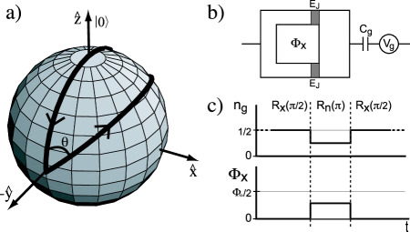
Figure 1: a) Evolution of the Bloch vector on the Bloch sphere for the sequence of pulses (8). The initial (cyclic) state vector is $|0\rangle$. Starting with $|1\rangle$ yields a similar path but centered on the south pole of the Bloch sphere. b) Symmetric charge qubit. The control parameters are the gate voltage $V_{g}$ and the external flux $\Phi_{x}$. c) Sequence of external flux $\Phi_{x}$ and dimensionless gate charge $n_{g}$ implementing $R_{z}^{AA}(\theta)$. The gate charge is related to the gate voltage by $n_{g}=C_{g}V_{g}/2e$. Relative amplitude of flux and gate voltage during $R_{n}(\pi)$ is used to tune $\theta$, see Fig. 2.

If one can turn on and tune the coefficients of $\sigma_{x}$ and $\sigma_{z}$ simultaneously, the following evolution is possible

$$R_{z}^{AA}(\theta)\equiv R_{x}(\pi/2)R_{\mathbf{n}}(\pi)R_{x}(\pi/2),$$ (8)

with $\mathbf{n}=(-\cos\theta,\mathrm{0},\sin\theta)$ and $B_{n}=\sqrt{B_{x}^{2}+B_{z}^{2}}$. This operation acts as $R_{z}^{AA}(\theta)\>|0\rangle=e^{-i\,\theta}\>|0\rangle$. Figure 1a) is a plot of this path on the Bloch sphere. Since this path satisfies Eq.(6), the dynamic phase is zero for this evolution and, as a result, the geometric AA phase is just $-\theta$. By varying the angle of the axis of rotation $\theta$, it is possible to obtain any geometric phases. Incidentally, in implementations for which the fields $B_{x}$ and $B_{z}$ cannot be non-zero simultaneously, one is restricted to $\mathbf{n}=\pm\mathbf{z}$ and hence to multiples of $\pi/2$ for $\theta$.

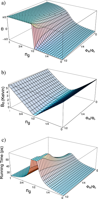
Figure 2: a) Possible values of the geometric phase $\theta=\arctan[2E_{c}\left(2n_{g}-1\right)/E_{J}\cos\left(\pi\Phi_{x}/\Phi_{0}\right)]$ for the symmetric superconducting charge qubit as a function of gate charge $n_{g}$ and external flux $\Phi_{x}$ of the rotation $R_{\mathbf{n}}(\pi)$. The characteristic energies of the qubit are chosen as in Ref. nakamura:99 : $E_{J}=0.6$K and $E_{c}=1.35$K. The relative phase $2\theta$ can be chosen in the full range $[0,2\pi]$ by an appropriate choice of the control parameters. b) Magnitude of the effective field $B_{n}$ as a function of the external parameters. c) Total running time of $R_{z}^{AA}(\theta)$ (in picoseconds) as a function of external control parameters of the $R_{n}\left(\pi\right)$ operation in Eq. (8). We assume that the $R_{x}\left(\pi/2\right)$ part of the operation is performed at the fastest possible rate. Due to limitations of voltage and current (i.e. flux) pulse generators, actual running time may be larger nakamura:99 . Finite rise time of the pulses was not taken into account.

This operation can be implemented, for example, with a symmetric superconducting charge qubit makhlin:2001 , Figure 1b), by using the sequence of flux and gate voltage of Figure 1c). This is similar to what was suggested recently in Ref. xiangbin:2001 . Figure 2a) and 2b) show respectively the angle $\theta$ and the magnitude of the effective field $B_{n}$ for $R_{\mathbf{n}}(\pi)$ as a function of gate voltage and external flux applied on the charge qubit. Here, $B_{z}=4E_{c}(1-2n_{g})$ and $B_{x}=2E_{J}\cos(\pi\Phi_{x}/\Phi_{0})$ where $\Phi_{0}=h/2e$ is the flux quantum and $E_{c}$ and $E_{J}$ are respectively the charging and Josephson energies makhlin:2001 . Because of the dependence of $B_{n}$ on the external parameters, the time $t_{n}=\pi/B_{n}$ required to implement $R_{\mathbf{n}}(\pi)$ depends on the desired geometric phase $\theta$, Figure 2c).

The gate sequence (8) on the superposition $(a|0\rangle+b|1\rangle)/\sqrt{2}$ yields

$$\frac{1}{\sqrt{2}}\left(a\,e^{-i\,\theta}\,|0\rangle+b\,e^{+i\,\theta}\,|1\rangle\right)$$ (9)

and the phase difference between $|0\rangle$ and $|1\rangle$ has observable consequences. While this final state depends on the AA phase of the evolution of $|0\rangle$ and $|1\rangle$ separately, it is not a cyclic evolution when acting on their superposition.

For the adiabatic (Berry) phase, a similar situation does not cause any ambiguities. In that case, as stated earlier, a superposition of eigenstates does not yield a cyclic evolution for the state vector either. Nevertheless, the phase acquired by each eigenstate still has a contribution which is geometric in nature since cyclicity is not required in projective space but in the Hamiltonian parameter space anandan:87b .

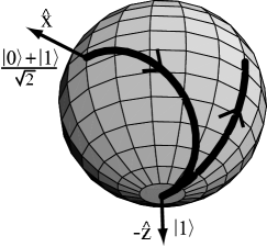
Figure 3: The sequence of rotations (8) applied on the superposition of states $(|0\rangle+|1\rangle)/\sqrt{2}$ does not yield a closed path on the Bloch sphere.

In the non-adiabatic case however, there is clearly no closed loop on the Bloch sphere, as shown on Figure 3, and identifying the AA phase according to Aharonov and Anandan’s original definition is more subtle. This situation has suggested to some authors bouchiat:88 that the AA phase is not observable for any evolution on an isolated quantum system. The reason is that the AA phase is defined only for cyclic evolutions and, since global phase factors are not physical, observable properties are unchanged for such evolutions.

While a non-abelian version of the non-adiabatic phase can be defined and the phase factors in (9) can be seen as geometric anandan:88 , a direct observation of the AA phase as in the NMR experiment of Suter et al. suter:88 is interesting but will require more than one qubit. In the language of quantum computation, the analog of this NMR experiment is to use a second qubit to ‘monitor’ the phase on the first one. Explicitly, start with a two-qubit state assuming the first qubit is in an arbitrary linear superposition

$$(a|0\rangle+b|1\rangle)\;|0\rangle.$$ (10)

Then, apply the sequence (8) on the second qubit, conditionally on the first qubit to be $|1\rangle$

$$\begin{split}C_{R_{z}^{AA}}&\equiv C_{\mathrm{NOT}}\,R_{z2}^{AA}(-\theta/2)\,C_{\mathrm{NOT}}\,R_{z2}^{AA}(\theta/2)\\ &=\begin{pmatrix}1&&&\\ &1&&\\ &&e^{-i\theta}&\\ &&&e^{+i\theta}\end{pmatrix}.\end{split}$$ (11)

The operation $C_{\mathrm{NOT}}$ is the Controlled-NOT applied on the two qubits, the first one acting as control. $R_{z2}^{AA}(\pm\theta/2)$ is (8) applied on qubit 2 only. This yields

$$\begin{split}C_{R_{z}^{AA}}\>(a|00\rangle+b|10\rangle)&=a|00\rangle+be^{-i\,\theta}|10\rangle\\ &=(a|0\rangle+e^{-i\,\theta}b|1\rangle)\;|0\rangle.\end{split}$$ (12)

The net result is equivalent to a geometric phase gate on the first qubit. It can be observed from the first qubit by interference neutron . There is no ambiguity in defining the AA phase in this situation : The second qubit undergoes a cyclic evolution and its phase is measurable since the evolution of the total system is not cyclic.

The controlled-NOT can be realized as

$$C_{\mathrm{NOT}} = e^{-i3\pi/4}\,R_{x2}(3\pi/2)\,C_{P}(3\pi/2)\,R_{z2}(\pi/2)$$ (13)

$$R_{x2}(\pi/2)\,R_{z2}(\pi/2)\,R_{z1}(\pi/2)\,C_{P}(3\pi/2).$$

This particular sequence is specific to quantum computer implementations having the control phase shift gate

$$C_{P}(\gamma)=e^{-i\gamma\,\sigma_{z}\otimes\sigma_{z}/2}$$ (14)

in their repertory but similar sequences can be found for other implementations. For the charge qubit, such a $\sigma_{z}\otimes\sigma_{z}$ interaction can be implemented by capacitive coupling falci:2000 .

Using (8) and (13), it is possible by inspection to ‘compile’ the total sequence (11) from $2\times(7+3)=20$ down to $18$ elementary operations. Moreover, one can verify that the dynamic phase cancels in (11). This therefore corresponds to a purely geometric 2-qubit operation. This logic gate however involves the application of $18$ elementary gates, a number that is quite large for a gate whose purpose is to implement a “noiseless” (geometric) phase-shift gate.

III Tolerance to noise in control parameters

A central issue to address in a pragmatic way is tolerance to imperfections. If non-adiabatic geometric logical gates are to be useful for computation, there should be some tolerance to fluctuations in the control parameters. Fluctuations of the control fields will introduce imperfections in the angles and axes of rotation of the gates implementing the geometric evolution. These imperfections change the overall unitary evolution applied on the qubit and the corresponding final phase may now have a dynamic component. It is important to note that whether the imperfections affect the dynamic or the geometric component is not relevant for our analysis. Any unwanted phase factor represents an error on the quantum computation. In the following, we thus focus on the errors on the total phase coming from fluctuations in the control parameters around the values that are needed to achieve the desired unitary transformations in the non-fluctuating case.

Let us consider first the effect of the simplest of such errors: an error $\epsilon$ in the angle of the first gate of the sequence (8)

$$R_{x}(\pi/2)R_{\mathbf{n}}(\pi)R_{x}(\pi/2+\epsilon).$$ (15)

We do not consider the extra gates (11) for the moment. Evidently, this is not an area preserving error and one should not expect the AA phase to be invariant in this circumstance. However, this is exactly the type of errors which will occur if the control field $B_{x}(t)$ is fluctuating.

That the non-adiabatic phase gate is not tolerant to this error is easily checked by applying the erroneous sequence (15) on the state $|0\rangle$ to obtain

$$\cos(\epsilon/2)\,e^{-i\,\theta}\,|0\rangle-i\sin(\epsilon/2)\,e^{+i\theta}\,|1\rangle.$$ (16)

The evolution is not cyclic anymore and we cannot define the AA phase in this situation (at least not in the computational basis). Note that to first order in $\epsilon$, the non-cyclicity remains and therefore non-adiabatic phase gates are not tolerant to small imperfections. Small errors can take the state vector out of great circles and bring in a dynamical contribution. In worse cases, as above, the evolution is no longer cyclic and the AA phase can no longer be defined in the computational basis.

It is possible to get a more complete picture of the effect of random noise on the non-adiabatic phase gate and see how it compares to the simpler dynamic phase gate

$$R_{z}(\theta)=e^{-i\theta\>\sigma_{z}/2}$$ (17)

by studying the Hamiltonian

$$H=\frac{1}{2}\sum_{i=x,z}(B_{i}(t)+\delta B_{i}(t))\,\sigma_{i}.$$ (18)

Here, $\delta B_{i}$ represents fluctuations of the control field $B_{i}$. It is believed that fluctuations of the control fields are the most damaging sources of noise and decoherence for solid-state qubits makhlin:2001 . For the charge qubit of Figure 1b), this corresponds to Nyquist-Johnson noise in the gate voltage $V_{g}$ and in the current generating the flux $\Phi_{x}$.

Without noise, $R_{z}^{AA}(\theta/2)$ and $R_{z}(\theta)$ have the same effect. To compare these gates in the presence of noise, we simply use the composition property of the evolution operator

$$U(t)=\mathcal{T}\>e^{-i\int_{0}^{t}\,dt^{\prime}H(t^{\prime})}=\lim_{N\rightarrow\infty}\prod_{n=1}^{N}U(n),$$ (19)

where $U(n)=\exp{(-iH(n)\,t/N)}$ and $H(n)$ is the Hamiltonian during the $n^{\mathrm{th}}$ interval. We use units where $\hbar=1.$ To simulate noise, the fields $\delta B_{i}(n)$ are chosen as independent random variables drawn from a uniform probability distribution in the interval $\pm\delta B_{max}$. Without noise, the decomposition (19) is of course exact, whatever the value of $N$, since the logical operations $R_{z}^{AA}(\theta/2)$ and $R_{z}(\theta)$ are implemented by piecewise constant Hamiltonians. With noise, we assume that the $\delta B_{i}$ are time independent during the interval $\Delta t\equiv t/N_{i}$. We then define $\Delta t$ as the noise correlation time. It will be assumed to be the same during the application of any elementary operation $R_{i}.$ With the decomposition of Eq. (19), the evolution is explicitly unitary.

To compare the two operations, we compute the trace distance nielsen-chuang

$$D(U,V)=\mathrm{Tr}\left\{\sqrt{(U-V)^{{\dagger}}(U-V)}\right\}$$ (20)

with respect to the noiseless $R_{z}(\theta)$ gate. We reached the same conclusions when the average fidelity nielsen:2002 was used numerically to compare noisy and noiseless gates. The trace distance $D(U,V)$ takes values between 0 and 4, with $D(U,V)=0$ only for $U$ and $V$ equal. Thus, if the non-adiabatic gate is to be more tolerant to noise than its dynamic counterpart then

$$D\boldsymbol{(}\tilde{R}_{z}^{AA}(\theta/2),R_{z}(\theta)\boldsymbol{)}<D\boldsymbol{(}\tilde{R}_{z}(\theta),R_{z}(\theta)\boldsymbol{)}$$ (21)

should hold. The tilde is used here to denote noisy logical gates.

To compute the distance, we expand $U(n)$ in (19) to first order in $\delta B$ and $t/N$ and average the distance obtained from this approximation by applying the Central Limit Theorem to the variables $X_{i}\equiv\sum_{i=1}^{N}\delta B_{i}\left(n\right)$. In addition, we note that the time necessary to complete $R_{i}\left(\phi\right)$ is $t_{i}=N_{i}\Delta t=\phi/B_{i}$. For the geometric gate, this leads to $N_{n}B_{n}=2N_{x}B_{x}$ since the rotation angles involved in Eq. (8) are $\pi$ and $\pi/2$ respectively. In this way, we obtain in the presence of noise along $x$ and $z$

$$\langle D\boldsymbol{(}\tilde{R}_{z}^{AA}(\theta/2),R_{z}(\theta)\boldsymbol{)}\rangle \approx \sqrt{\frac{\pi^{3}}{12}\left(\frac{1}{B_{x}^{2}}+\frac{1}{B_{x}B_{n}}\right)}\frac{\delta B_{\mathrm{max}}}{\sqrt{N_{x}}};$$

$$\langle D\boldsymbol{(}\tilde{R}_{z}(\theta),R_{z}(\theta)\boldsymbol{)}\rangle \approx \sqrt{\frac{\pi}{6}}\,\frac{\theta\,\delta B_{\mathrm{max}}/B_{z}}{\sqrt{N_{z}}},$$ (22b)

where $$B_{x} B_{n} B_{z} R_{x}(\pi/2) R_{\mathbf{n}}(\pi) R_{z}(\theta) N_{i} N_{i}$$, and are the magnitudes of the effective fields used to implement respectively , and . As gets smaller, the noise is constant on a larger portion of the evolution and excursions on the Bloch sphere farther away from the original path are possible. The distance between the noisy and noiseless gates therefore increases as diminishes.

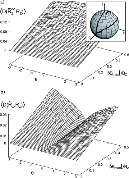
Figure 4: Trace distance as a function of $\theta$ and maximum amplitude of the noise averaged over 600 realizations of the noise. Noise is along $x$ and $z$ and is in units of the maximal value of the effective field in the $z$ direction $B_{z}=4E_{c}$. a) Averaged trace distance between a noisy AA-phase gate and the corresponding noiseless dynamic $R_{z}$ gate. The inset shows a path with random noise obtained from the numerical calculation. The path is not closed and the evolution is not cyclic. b) Similar to a) but for the noisy dynamic gate $R_{z}$. In both cases, the noise correlation time is taken as $\Delta t=\hbar/(4E_{c}\gamma)$ with $\gamma=300$. The charging and Josephson energies are taken as in Fig. 2.

Figure 4 shows a numerical verification of these relations. The weak dependence of $\langle D\boldsymbol{(}\tilde{R}_{z}^{AA}(\theta/2),R_{z}(\theta)\boldsymbol{)}\rangle$ on $\theta$ through $B_{n}$ is apparent in Fig. 4a). For $\langle D\boldsymbol{(}\tilde{R}_{z}(\theta),R_{z}(\theta)\boldsymbol{)}\rangle$, the dependence goes as $\sqrt{\theta}$ since $N_{z}\propto\theta$, Fig. 4b). The agreement between the analytical and numerical results was very good, with an error of about $3\%$ in both cases. Our first order estimates are then enough for this level of noise. Systems where the noise is of larger amplitude will most probably not be relevant for quantum computation so, for all practical purposes, this approximation should be enough.

Using the analytical estimates (22), the criterion (21), and taking the noise correlation time to be equal for dynamic and geometric gates, we obtain a bound on the angle $\theta$ beyond which the geometric gate becomes favorable over the dynamic one,

$$\theta_{b}>\pi\left(\frac{B_{z}}{B_{x}}+\frac{B_{z}}{B_{n}}\right).$$ (23)

Taking $B_{z}/B_{x}\approx B_{z}/B_{n}\approx 1$, we obtain that for $\theta_{b}\gtrsim 2\pi$ the geometric gate will be less affected by noise than its dynamic counterpart. For the charge qubit, $B_{z}$ and $B_{x}$ are fixed respectively by the charging energy $E_{c}$ and Josephson energy $E_{J}$. To encode efficiently information in the charge degree of freedom, the inequality $E_{C}\gg E_{J}$ must be satisfied makhlin:2001 . The bound obtained with $B_{z}/B_{x}\approx B_{z}/B_{n}\approx 1$ is therefore a lower bound on $\theta_{b}$. Since $\theta_{b}>2\pi$, the non-adiabatic geometric gate is never useful in practice. In particular, with the energies used in Fig. 2, we obtain $\theta_{b}\gtrsim 2.5\pi$ as a lower bound. More generally, since the logical states of a qubit are the eigenstates of $\sigma_{z}$, $B_{z}$ should be larger than $B_{x}$ for the logical basis to be the ‘good’ basis. We therefore expect this lower bound to hold for most quantum computer architectures.

We also obtained the analogs of the above results Eqs. (22) and (23) when the noise is along $z$ only and also found the geometric gate more sensitive to noise than the dynamical one.

The effect of decoherence on the AA phase gate was also studied numerically by Nazir et al. for non-unitary evolutions nazir:2002 . They reach the same conclusion on the sensitivity to noise of the AA phase gate. Since they can deal with more general noise than we do here, their approach is more general than ours but is entirely numerical. Our objective here was to include only the kind of noise to which geometric gates were previously suggested to be tolerant: unitary random noise about the path.

The approach used here to quantify the effect of fluctuations can be used for Berry’s phase gates as well. We consider the pulse sequence used in the NMR experiment of Ref. jones:2000 and simplified in nazir:2002 . The system Hamiltonian now takes the form

$$H=\frac{\Delta}{2}\,\sigma_{z}+\frac{\omega_{1}}{2}\left(\cos\phi\,\sigma_{x}+\sin\phi\,\sigma_{y}\right).$$ (24)

The sequence of operations used in Ref. jones:2000 starts with the field along the $z$ axis ($\omega_{1}=0$). The parameter $\Delta$ is assumed fixed throughout. The field is first adiabatically tilted in the $x$–$z$ plane by increasing $\omega_{1}$ at $\phi=0$ up to some maximal value $\omega_{1\,max}$. The field now makes an angle $\theta_{\mathrm{cone}}=\arccos(\Delta/\sqrt{\Delta^{2}+\omega_{1\,max}^{2}})$ with respect to the $z$ axis. With $\omega_{1}$ kept constant, $\phi$ is then adiabatically swept from $\phi=0$ to $\phi=2\pi$. To obtain a purely geometric operation, the dynamic phase is refocused by repeating the above operations in reverse between a pair of fast $R_{y}(\pi)$ rotations. The final relative phase is then purely geometric and has the value $\gamma=4\pi(1-\cos\theta_{\mathrm{cone}})$ jones:2000 .

To study the effect of noise for this sequence, we again use the composition property (19) and a Trotter decomposition for (24). In the same way as above, we then obtain in the case of noise along $x$, $y$, and $z$ and assuming that the $R_{y}(\pi)$ rotations are noiseless,

$$\langle D\boldsymbol{(}\tilde{R}_{z}^{Berry}(\gamma),R_{z}(\gamma)\boldsymbol{)}\rangle\approx\frac{4}{\sqrt{3\pi}}\,\delta B_{\mathrm{max}}\,\sqrt{\frac{T_{T}^{2}}{N_{T}}+\frac{T_{\phi}^{2}}{N_{\phi}}},$$ (25)

where $T_{T}$ is the time taken to tilt the field in the $x$–$z$ plane and $T_{\phi}$ the time for the $\phi$ sweep. As in (22), the larger $N_{T}$ and $N_{\phi}$ are, the smaller is the noise correlation time. Agreement of this result with numerical calculations (not shown) is excellent. The adiabaticity constraint means that $T_{T}$ and $T_{\phi}$ must be large and therefore that, for all practical purposes, the Berry’s phase gate is worse than its dynamic equivalent. The conclusion is the same for all the different types of noise tested numerically. For the $\omega_{1}$ tilt, these are noise along $x$ only and uncorrelated noise along $x$ and $z$. For the $\phi$ sweep, we took identical noise along $x$ and $y$, and tested its effect with and without uncorrelated noise along $z$. Because of the adiabatic constraint, the Berry’s phase gate is also worse than the AA phase gate. This is the conclusion reached as well in Ref. nazir:2002 in the case of non-unitary evolutions. The possibility ekert:2000 to find a point of operation where conditional phase shifts are insensitive, to linear order, to noise in $\omega_{1}$ $\left(B_{x}\right)$ may however, in very special cases, be an advantage of Berry-phase gates for coupled qubits.

The overall results of this section can be understood intuitively rather simply. To implement logical gates that use geometric phases (adiabatic or not), one needs to apply a sequence of unitary transformations that take the Bloch vector around a closed path. In the presence of noise in the control fields, that sequence does not take the Bloch vector around a closed path anymore. Since all that counts is the overall phase of the unitary transformation, this phase will be more affected in the long sequences of unitary transformations necessary for geometric gates than in the shorter sequences necessary for purely dynamical gates. We may point out that if the noise has a special symmetry that makes it area preserving, then this symmetry might allow quantum error correction steane:99 , decoherence-free subspaces zanardi:97 ; lidar:98 or bang-bang techniques viola:98 to be used with more success than geometric gates.

IV Conclusion

In summary, we have considered the AA phase as a tool for quantum computation. This phase solves many of the problems of Berry’s phase gate. Namely, it can be implemented faster, does not require refocusing of a dynamic component and involves control over only two effective fields in the one-qubit Hamiltonian. We showed how the AA phase of one qubit can be monitored by a second qubit without extra dynamical phase. As an example, details of the implementation of the AA phase with a symmetric charge qubit were given. Application of these ideas to other quantum computer architectures is a simple generalization.

When the effect of noise in the control parameters is taken into account, it appears that practical implementations of logical gates based on geometric phase ideas, both adiabatic and non-adiabatic, are more sensitive to noise than purely dynamic ones, contrary to what was previously claimed. We have checked how noise affects the overall unitary transformations that, in the noiseless case, implement purely geometric logical gates. The analytical results were confirmed numerically and for a wide range of noise symmetries. This is in agreement with the recent work of Ref. nazir:2002 . In the present work however, we focused our attention on the type of noise to which the geometric logical gates were previously assumed to be tolerant.

The use of the AA phase for quantum computation purposes therefore seems to be of little practical interest. It is however of fundamental interest to observe this phase and a direct observation with the symmetric superconducting charge qubit seems possible.

- (1) D. Vion, A. Aassime, A. Cottet, P. Joyez, H. Pothier, C. Urbina, D. Esteve and M.H. Devoret, Science 296, 886 (2002).
- (2) A.M. Steane, in Introduction to Quantum Computation and Information, edited by H.K. Lo, S. Popescu and T.P. Spiller (World Scientific, Singapore, 1999), p. 184.
- (3) P. Zanardi and M. Rasetti, Phys. Rev. Lett. 79, 3306 (1997).
- (4) D.A. Lidar, I.L. Chuang and K.B. Whaley Phys. Rev. Lett. 81, 2594 (1998).
- (5) L. Viola and S. Lloyd Phys. Rev. A 58, 2733 (1998).
- (6) M.V. Berry, Proc. R. Soc. Lond. A392, 45 (1984).
- (7) J. Jones, V. Vedral, A. Ekert and G. Castagnoli, Nature 403, 869 (2000).
- (8) A. Ekert, M. Ericsson, P. Hayden, H. Inamori, J.A. Jones, D.K.L. Oi and V. Vedral, Journal of Modern Optics 47, 2501 (2000).
- (9) G. Falci, R. Fazio, G. Massimo Palma, J. Siewert and V. Vedral, Nature 407, 355 (2000).
- (10) F. Wilczek and A. Zee Phys. Rev. Lett. 52, 2111 (1984).
- (11) P. Zanardi and M. Rasetti Phys. Lett. A 264, 94 (1999).
- (12) L.-M. Duan, J.I. Cirac and P. Zoller Science 292, 1965 (2001).
- (13) M.-S. Choi, quant-ph/0111019 (2001).
- (14) L. Faoro, J. Siewert, R. Fazio, cond-mat/0202217 (2002).
- (15) Y. Aharonov and J. Anandan, Phys. Rev. Lett. 58, 1593 (1987).
- (16) W. Xiang-Bin and M. Keiji, quant-ph/0104127 (2001); W. Xiang-Bin and M. Keiji, Phys. Rev. B 65, 172508 (2002).
- (17) Y. Makhlin, G. Schön, and A. Shnirman, Rev. Mod. Phys. 73, 357 (2001).
- (18) J. Anandan and L. Stodolsky, Phys. Rev. D 35, 2597 (1987).
- (19) D. Bacon, J. Kempe, D.P. DiVincenzo, D.A. Lidar and K.B. Whaley, in Proceedings of the 1st International Conference on Experimental Emplementations of Quantum Computation, Sydney, Australia, edited by R. Clark (Rinton, Princeton, NJ, 2001), p. 257. quant-ph/0102140.
- (20) D.J. Moore, Phys. Rep. 210, 1 (1991).
- (21) Y. Nakamura, Y.P. Pashkin and J.S. Tsai, Nature 398, 786 (1999).
- (22) C. Bouchiat and G.W. Gibbons J. Phys. 49, 187 (1988).
- (23) J. Anandan Phys. Lett. A 133, 171 (1988).
- (24) D. Suter, K.T. Mueller and A. Pines, Phys. Rev. Lett. 60, 1218 (1988).
- (25) This is equivalent, for example, to a neutron interferometry experiment where the first qubit in Eq.(10) represents position and the second spin of the neutron. Since a qubit has only, by construction, a two-dimensional Hilbert space, it is necessary to use more then one qubit to mimic interferometry experiments where more than one degree of freedom of a single particle are used.
- (26) M.A. Nielsen and I.L. Chuang Quantum Computation and Quantum Information, (Cambridge University Press, 2000).
- (27) M D. Bowdrey, D.K.L. Oi, A.J. Short, K. Banaszek, and J.A. Jones, Phys. Lett. A 294, 258 (2002); M.A. Nielsen, quant-ph/0205035 (2002);
- (28) A. Nazir, T.P. Spiller and W.J. Munroe, Phys. Rev. A 65, 042303 (2002).