Ponderomotive entangling of atomic motions

Abstract

We propose the use of ponderomotive forces to entangle the motions of different atoms. Two situations are analyzed: one where the atoms belong to the same optical cavity and interact with the same radiation field mode; the other where each atom is placed in own optical cavity and the output field of one cavity enters the other.

I Introduction

The preparation of entangled atomic states is one of the goals of atomic physics and quantum optics. These states are the key ingredients for studying some fundamental issues of quantum mechanics [1], as well as for certain applications related to quantum information [2]. Various methods have been recently proposed to engineer entanglement between atoms [3, 4, 5]. They are based on achieving and controlling an effective interaction between the atoms that are to be entangled. Typically, these interactions are mediated by the electromagnetic field, but also involve transitions between internal atomic states.

On the other hand, atoms and radiation fields can interact via radiation pressure effects. The role of such ponderomotive effects in probing fundamental aspects of quantum theory has been pointed out in a number of recent papers [6, 7]. Here we shall exploit ponderomotive effects to propose a method of entangling atomic motions. This is fundamentally important as radiation pressure effects are universal and scalable. For example, radiation pressure effects could also be fruitful in entangling massive particles (or even macroscopic objects). If such a scheme happens to be successful for atoms, one would acquire the confidence of trying out a similar scheme with more massive objects. Another advantage of a ponderomotive scheme becomes clear when we note that most existing mechanisms for entangling atoms, apart from a very few [5], entangle internal atomic states. As such, the maximum degree of entanglement attainable is limited by the finite dimensionality of the Hilbert space of the internal states of the interacting atoms. Our scheme, on the other hand, entangles atomic motions and therefore entangles two continuous variable (infinite dimensional) systems. Moreover, as we shall demonstrate, our entangling mechanism, in contrast to most others, does not require carefully controlled switching on and off of external laser fields acting on the individual atoms.

As Hamiltonian model, we shall consider the case of large detuning of internal atomic transitions from the cavity field so that spontaneous emission can be neglected and the upper atomic level can be adiabatically eliminated [8]. In this case, the atom-field interaction reduces to the product between the number of photons and the amplitude of atomic displacement. The atomic internal states are never involved in the interaction and the atom can always stay in a fixed internal ground state.

II Atoms in the same optical cavity

We first consider two trapped atoms $A$ and $B$ in the same optical cavity. When they are invested by the (off-resonant) laser light, the evolution in one spatial direction takes place according to the Hamiltonian (in natural units)

$$H=\chi c^{{\dagger}}c\left(a+a^{\dagger}+b+b^{\dagger}\right)+\Omega(a^{\dagger}a+b^{\dagger}b)\,$$ (1)

where $a,b$ and $c$ are annihilation operators for the vibrational motion of the two atoms and the cavity mode respectively. Furthermore, $\Omega$ is the vibrational frequency (assumed equal for the two atoms). The time evolution operator corresponding to the Hamiltonian (1) can be put in the following form [6]

$$U(t) = \exp\left[2i\kappa^{2}\left(c^{{\dagger}}c\right)^{2}\left(t-\sin t\right)\right]$$ (5)

$$\times\exp\left[\kappa c^{{\dagger}}c\left(\eta(t)a^{{\dagger}}-\eta^{*}(t)a\right)\right]$$

$$\times\exp\left[\kappa c^{{\dagger}}c\left(\eta(t)b^{{\dagger}}-\eta^{*}(t)b\right)\right]$$

$$\times\exp\left[-it\left(a^{{\dagger}}a+b^{{\dagger}}b\right)\right]\,,$$

where $\eta(t)=(1-e^{-it})$, $\kappa=\chi/\Omega$ and the time is scaled accordingly to $\Omega t\to t$.

Let us now assume that initially both atoms are cooled down to their ground states and the cavity field is in coherent states, that is

$$|\Psi(0)\rangle=|0\rangle_{a}\otimes|0\rangle_{b}\otimes|\zeta\rangle_{c}\,,$$ (6)

then, the time evolution leads to

$$|\Psi(t)\rangle = e^{-|\zeta|^{2}/2}\sum_{n=0}^{\infty}\frac{\zeta^{n}}{\sqrt{n!}}e^{2i\kappa^{2}n^{2}(t-\sin t)}$$ (8)

$$|n\kappa\eta(t)\rangle_{a}\otimes|n\kappa\eta(t)\rangle_{b}\otimes|n\rangle_{c}\,,$$

where $|n\kappa\eta(t)\rangle_{a,b}$ are coherent states of the atoms.

Let us suppose to measure the quadrature $X=(c+c^{{\dagger}})/\sqrt{2}$. Then the state after the measurement will be

$$|{\widetilde{\Psi}}(t)\rangle={\cal N}\,|x\rangle_{c}{}_{c}\langle x|\Psi(t)\rangle\,,$$ (9)

where ${\cal N}$ is a normalization constant, while $|x\rangle$ are the eigenvectors of the quadrature observable $X$. The inverse of normalization constant also gives the probability amplitude of the outcome $x$, that is $P(x)={\cal N}^{-2}$.

The joint state of the atoms after the measurement results

$$|\widetilde{\Psi}(t)\rangle = {\cal N}e^{-|\zeta|^{2}/2}\sum_{n=0}^{\infty}\frac{\zeta^{n}}{\sqrt{n!}}e^{2i\kappa^{2}n^{2}(t-\sin t)}{}_{c}\langle x|n\rangle_{c}$$ (11)

$$|n\kappa\eta(t)\rangle_{a}\otimes|n\kappa\eta(t)\rangle_{b}\,,$$

where

$${}_{c}\langle x|n\rangle_{c}=\pi^{-1/4}(2^{n}n!)^{-1/2}H_{n}(x)\exp(-x^{2}/2)\,,$$ (12)

are the harmonic oscillator position eigenstates, with $H_{n}$ the Hermite polynomials.

The state (11) depends on the time at which the measurement is performed and is conditioned to the result $x$ of the measurement. Let us choose a time $t_{N}=(2N+1)\pi$ with $N\in{\bf N}$, so that $\eta(t_{N})=2$, and $\kappa\in{\bf N}$, thus Eq.(11) becomes

$$|\widetilde{\Psi}(t_{N})\rangle={\cal N}e^{-|\zeta|^{2}/2}\sum_{n=0}^{\infty}\frac{\zeta^{n}}{\sqrt{n!}}\,{}_{c}\langle x|n\rangle_{c}\,|4\kappa n\rangle_{a}\otimes|4\kappa n\rangle_{b}\,.$$ (13)

It is clear that the above state represent an entangled state for the atoms. In practice, since the radiation field mediates information between the two atoms, a measurement of its quadrature leaves the atoms correlated.

In order to quantify the degree of entanglement we calculate the linear entropy [9]

$$E=1-{\rm Tr}_{a}\{[{\rm Tr}_{b}(\,\widetilde{\rho}\,)]^{2}\}\,,$$ (14)

where $\widetilde{\rho}=|\widetilde{\Psi}(t_{N})\rangle\langle\widetilde{\Psi}(t_{N})|$. However, since the formation of entangled states is conditioned to the measurement on the radiation field, it would be useful to define the efficiency of the entanglement procedure as

$$\Upsilon(x)=E(x)\times P(x)\,.$$ (15)

Then, in Fig.1 we show the efficiency $\Upsilon$ as function of quadrature outcome $x$. We clearly see that the efficiency increases as the radiation pressure (i.e., the amplitude of the radiation field) increases. The shape of $\Upsilon$ comes from the fact that $x=0$ is the most probable outcome of the measurement, but the entanglement has a minimum at that value.

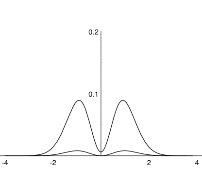
FIG. 1.: Entanglement efficiency vs quadrature outcome for different values of $\zeta$ (from bottom to top, $\zeta=0.1$, $0.4$, $0.8$). Here, $\kappa=1$.

Note that by increasing $\kappa$ sufficiently, the set of states $\{|4\kappa n\rangle\}$ in Eq.(13) can be made to approach an orthonormal basis arbitrarily close. This means that we can approach the maximal entanglement possible in any $D\times D$ system arbitrarily closely by setting the field amplitude $\zeta$ to a required value and increasing $\kappa$. For example, for a $10\times 10$ system, the maximum entanglement according to the measure of Eq.(14) is $0.9$. This is already exceeded for a field amplitude $\zeta=6$. The above fact clearly illustrates one of the advantages of entangling through our scheme in contrast to entangling the internal levels of two two-level atoms as in most existing schemes. The degree of entanglement achievable is not bounded from above by any fundamental constraint. Of course, the degree of entanglement one can practically produce will depend on parameters such as the Q-factor of the cavity in a specific experimental realization.

III Atoms in distinct optical cavities

We now consider the two (trapped) atoms placed in separate cavities, and interacting sequentially with the same radiation field. That is, the outgoing field from the first cavity enters the second one. Therefore, the Hamiltonian (1) should be modified as follows:

$$H = \chi c_{1}^{{\dagger}}c_{1}(a+a^{{\dagger}})+\chi c_{2}^{{\dagger}}c_{2}(b+b^{{\dagger}})$$ (17)

$$+\Omega(a^{{\dagger}}a+b^{{\dagger}}b)\,,$$

where we have assumed the same coupling constant and the same oscillatory frequency for the two atoms.

However, in such a case we have to consider photon losses, which we assume to occour at same rate $\gamma$ in the two cavities. We further assume a decay of the atomic motions at rate $\Gamma$. Thus, we can write down the quantum Langevin equations as

$${\dot{a}} = -i\Omega a-i\chi c_{1}^{{\dagger}}c_{1}-\frac{\Gamma}{2}a+\sqrt{\Gamma}a^{in}\,,$$ (18)

$${\dot{b}} = -i\Omega b-i\chi c_{2}^{{\dagger}}c_{2}-\frac{\Gamma}{2}b+\sqrt{\Gamma}b^{in}\,,$$ (19)

$${\dot{c}_{1}} = -i\Delta_{1}c_{1}-i\chi c_{1}(a+a^{{\dagger}})-\frac{\gamma}{2}c_{1}+\sqrt{\gamma}c_{1}^{in}\,,$$ (20)

$${\dot{c}_{2}} = -i\Delta_{2}c_{2}-i\chi c_{2}(b+b^{{\dagger}})-\frac{\gamma}{2}c_{2}+\sqrt{\gamma}c_{2}^{in}\,,$$ (21)

where all the input operators represent vacuum noise [10]. $\Delta_{1}$ and $\Delta_{2}$ are the cavity detunings. The boundary condition reads

$$c_{2}^{in}\equiv c_{1}^{out}=\sqrt{\gamma}c_{1}-c_{1}^{in}\,.$$ (22)

To solve the system of Eqs.(18), (19), (20), (21), we proceede by the linearization around the steady state. The latter is characterized by

$$\zeta_{j}\left\{\frac{\gamma}{2}+\frac{\chi^{2}|\zeta_{j}|^{2}\Gamma}{\frac{\Gamma^{2}}{4}+\Omega^{2}}\right.$$ (23)

$$\qquad\left.+i\left[\Delta_{j}-2\frac{\chi^{2}|\zeta_{j}|^{2}\Omega}{\frac{\Gamma^{2}}{4}+\Omega^{2}}\right]\right\}=\sqrt{\gamma}\zeta_{j}^{in}\,;j=1,2\,,$$ (24)

with the relation

$$\zeta_{2}^{in}\equiv\zeta_{1}^{out}=\sqrt{\gamma}\zeta_{1}-\zeta_{1}^{in}\,.$$ (25)

Here, $\zeta$ is the steady state value of the operators $c$, and $\zeta_{1}^{in}$ is the amplitude of the input field (at the first cavity). Eq.(23) shows a typical bistable behavior [11]. Furthermore, the steady states of atomic operators $a$ and $b$ are given by

$$\alpha = -i\frac{\chi}{\frac{\Gamma}{2}+i\Omega}|\zeta_{1}|^{2}\,,$$ (26)

$$\beta = -i\frac{\chi}{\frac{\Gamma}{2}+i\Omega}|\zeta_{2}|^{2}\,.$$ (27)

The linearized system of equations can be written in the frequency domain as

$$i\omega\tilde{v}={\cal M}\tilde{v}+\tilde{v}_{in}$$ (28)

where the transposed vectors $\tilde{v}^{T}$ and $\tilde{v}_{in}^{T}$ are given by

$$\tilde{v}^{T}=(\tilde{a},\tilde{a}^{{\dagger}},\tilde{b},\tilde{b}^{{\dagger}},\tilde{c}_{1},\tilde{c}_{1}^{{\dagger}},\tilde{c}_{2},\tilde{c}_{2}^{{\dagger}})\,,$$ (29)

and

$$\tilde{v}_{in}^{T} = (\sqrt{\Gamma}\tilde{a}_{in},\sqrt{\Gamma}\tilde{a}_{in}^{{\dagger}},\sqrt{\Gamma}\tilde{b}_{in},\sqrt{\Gamma}\tilde{b}_{in}^{{\dagger}},$$ (31)

$$\sqrt{\gamma}\tilde{c}^{in}_{1},\sqrt{\gamma}\tilde{c}_{1}^{in\,{\dagger}},-\sqrt{\gamma}\tilde{c}^{in}_{2},-\sqrt{\gamma}\tilde{c}_{2}^{in\,{\dagger}})\,,$$

where now all the operators represent small quantum fluctuations around steady state. Moreover, the $8\times 8$ matrix ${\cal M}$ is

$${\cal M}=\left[\begin{array}[]{cc}M_{I}&M_{II}\\ M_{III}&M_{IV}\end{array}\right]$$ (32)

with

$$M_{I}=\left[\begin{array}[]{cccc}-\left(\frac{\Gamma}{2}+i\Omega\right)&0&0&0\\ 0&-\left(\frac{\Gamma}{2}-i\Omega\right)&0&0\\ 0&0&-\left(\frac{\Gamma}{2}+i\Omega\right)&0\\ 0&0&0&-\left(\frac{\Gamma}{2}-i\Omega\right)\end{array}\right]\,,$$ (33)

$$M_{II}=i\chi\left[\begin{array}[]{cccc}-\zeta_{1}^{*}&-\zeta_{1}&0&0\\ \zeta_{1}^{*}&\zeta_{1}&0&0\\ 0&0&-\zeta_{2}^{*}&-\zeta_{2}\\ 0&0&\zeta_{2}^{*}&\zeta_{2}\end{array}\right]\,;\quad M_{III}=i\chi\left[\begin{array}[]{cccc}-\zeta_{1}&-\zeta_{1}&0&0\\ \zeta_{1}^{*}&\zeta_{1}^{*}&0&0\\ 0&0&-\zeta_{2}&-\zeta_{2}\\ 0&0&\zeta_{2}^{*}&\zeta_{2}^{*}\end{array}\right]\,,$$ (34)

$$M_{IV}=\left[\begin{array}[]{cccc}-\frac{\gamma}{2}-i\left[\Delta_{1}+\chi\left(\alpha+\alpha^{*}\right)\right]&0&0&0\\ 0&-\frac{\gamma}{2}+i\left[\Delta_{1}+\chi\left(\alpha+\alpha^{*}\right)\right]&0&0\\ \gamma&0&-\frac{\gamma}{2}-i\left[\Delta_{2}+\chi\left(\beta+\beta^{*}\right)\right]&0\\ 0&\gamma&0&-\frac{\gamma}{2}+i\left[\Delta_{2}+\chi\left(\beta+\beta^{*}\right)\right]\end{array}\right]\,.$$ (35)

The solution of the Eq.(28) can formally be written as

$$\tilde{v}(\omega)=\left[i\omega{\cal I}-{\cal M}\right]^{-1}\tilde{v}_{in}(\omega)\,,$$ (36)

where ${\cal I}$ is the $8\times 8$ identity matrix. Then, the various frequency correlations can be easily calculated by using the correlations of the vacuum input noise [10]. These should deserve to quantify the entanglement of atomic motions. Nevertheless, since we deal with non pure states, it is very difficult to quantify the degree of entanglement [12]. To reach this goal we shall proceed as follows.

We first introduce the dimensionless atomic position and momentum variable

$$q_{a} = (a+a^{{\dagger}})\,,q_{b}=(b+b^{{\dagger}})\,,$$ (37)

$$p_{a} = -i(a-a^{{\dagger}})\,,p_{b}=-i(b-b^{{\dagger}})\,,$$ (38)

Now, if the atoms are entangled, one could infer position or momentum of one atom through position or momentum of the other [13]. The errors of these inferences are then quantified by the variances $\langle(q_{a}+q_{b})^{2}\rangle$ and $\langle(p_{a}-p_{b})^{2}\rangle$. Once the product of these inference errors lies below the limit of the Heisenberg principle, i.e. $\langle(q_{a}+q_{b})^{2}\rangle\dot{\langle}(p_{a}-p_{b})^{2}\rangle\leq|\langle[q_{a},p_{a}]\rangle|^{2}/4$, an EPR-like paradox arises [14]. This is a typical manifestation of the existence of purely quantum correlations between the two systems [13]. It is known that when $\langle(q_{a}+q_{b})^{2}\rangle\dot{\langle}(p_{a}-p_{b})^{2}\rangle$ is less than $1$ [15], the state is entangled irrespective of whether it is pure or mixed. Though the criteria for the presence of entanglement in continuous variable systems is present [15, 16], and we use this to prove the presence of entanglement in our case, there is as yet no rigorously proved measure of continuous variable entanglement. We shall use a quantity motivated from the above separability criterion to evaluate the degree of entanglement.

Now, given an operator $\tilde{\cal O}(\omega)$ in the frequency domain, we define the hermitian operator ${\cal R}_{\{\tilde{\cal O}\}}(\omega)=[\tilde{\cal O}(\omega)+\tilde{\cal O}(-\omega)]/2$. Then, recalling the previous argument, we can define the degree of entanglement as

$$E(\omega)=\frac{\langle{\cal R}^{2}_{\{\tilde{q}_{a}+\tilde{q}_{b}\}}(\omega)\rangle\,\langle{\cal R}^{2}_{\{\tilde{p}_{a}-\tilde{p}_{b}\}}(\omega)\rangle}{\frac{1}{4}\left|\langle\left[{\cal R}_{\tilde{q}_{a}}(\omega),{\cal R}_{\tilde{p}_{a}}(\omega)\right]\rangle\right|^{2}}\,,$$ (39)

which can be considered as a signature of entanglement whenever it goes below one. Notice that this condition is much stronger than the simple entanglement requirement, in that $E<1$ requires EPR-type correlations.

In Fig.2 we show the degree of entanglement (39) as function of the input field amplitude. The sharp decrement is due to the jump from one to the other branch of the bistable curve [11]. Then, by increasing the radiation intensity, the entanglement tends to disappear because of the increasing radiation pressure noise. In case of small coupling constant, entanglement effect appears at higher amplitudes (dashed line). Notice that we have used nonzero detunings to establish correlations between $q$ and $p$ variables, while naturally only $q$ variables tend to couple as results from Hamiltonian (17).

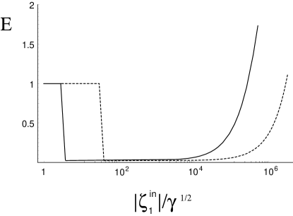
FIG. 2.: Degree of entanglement vs input field amplitude at frequency $\Omega$. The values of parameters (in unit of $\gamma$) are: $\chi=1$ (solid line), $\chi=0.1$ (dashed line) and $\Delta_{1}=\Delta_{2}=10^{4}$, $\Gamma=10^{-3}$.

IV Conclusions

In this paper we have discussed how to exploit radiation pressure effects to entangle the motions of two atoms. We have considered two scenarios: atoms in same and in separate cavities. As radiation pressure effects are very generic, the scheme should lead to those for more macroscopic objects. It also has the advantage of not involving either atomic internal states or various laser pulses being applied to the atoms. It is precisely this fact that offers the generality of our scheme, in the sense that it should not depend on the specific internal configuration of the atoms. Moreover, the entanglement between atoms in separate cavities is generated in the steady state (i.e. after all types of decoherence and dissipation have acted). This means that this type entanglement generating mechanism is robust in nature. Further generalizations of this scheme for entangling several atoms interacting with a common cavity field would be interesting and could potentially provide a simple way for generating multiparticle Schroedinger cat states.

REFERENCES

- [1] J. S. Bell, Physics 1, 195 (1965); J. F. Clauser, M. A. Horne, A. Shimony and R. A. Holt, Phys. Rev. Lett. 23, 880 (1969).
- [2] C. H. Bennett, Phys. Today 48(10), 24 (1995); D. P. DiVincenzo, Science 270, 255 (1995).
- [3] E. Hagley, X. Mantre, G. Nogues, C. Wunderlich, M. Brune, J. M. Raimond and S. Haroche, Phys. Rev. Lett. 79, 1 (1997); C. A. Sackett, D. Kielpinski, B. E. King, C. Langer, V. Meyer, C. J. Myatt, M. Rowe, Q. A. Turchette, W. M. Itano and D. J. Wineland, Nature 404, 256 (2000).
- [4] J. I. Cirac and P. Zoller, Phys. Rev. A 50, R2799 (1994); T. Pellizzari, S. Gardiner, J. I. Cirac and P. Zoller, Phys. Rev. Lett. 75, 3788 (1995); J. I. Cirac and P. Zoller, Phys. Rev. Lett. 74, 4091 (1995); J. F. Poyatos, J. I. Cirac and P. Zoller, Phys. Rev. Lett. 81, 1322 (1998); C. Cabrillo, J. I. Cirac, P. Garcia-Fernandez and P. Zoller, Phys. Rev. A 59, 1025 (1999); M.B. Plenio, S.F. Huelga, A. Beige and P.L. Knight, Phys. Rev. A 59 (1999) 2468; S. Bose, P. L. Knight, M. B. Plenio and V. Vedral, Phys. Rev. Lett. 83, 5158 (1999); A. Kuzmich and E. S. Polzik, Phys. Rev. Lett. 85, 5639 (2000); A. Beige, W. J. Munro and P. L. Knight, Phys. Rev. A 62 2102, (2000); S. Bose and D. Home, quant-ph/0101093.
- [5] A. S. Parkins, J. Opt. B.: Quant. Semiclass. Opt. 3, S18 (2001); A. S. Parkins and H. J. Kimble, Phys. Rev. A 61, 052104 (2000).
- [6] S. Mancini, V. I. Man’ko and P. Tombesi, Phys. Rev. A 55, 3042 (1997); S. Bose, K. Jacobs and P. Knight, Phys. Rev. A 56, 4175 (1997).
- [7] S. Bose, K. Jacobs and P. Knight, Phys. Rev. A 59, 3204 (1999); S. Mancini, D. Vitali and P. Tombesi, Phys. Rev. Lett. 80, 688 (1998); S. Mancini, Phys. Lett. A 279, 1 (2001); S. Mancini and A. Gatti, J. Opt. B.: Quant. Semiclass. Opt. 3, S66 (2001); V. Giovannetti, S. Mancini and P. Tombesi, Europhys. Lett. (to appear).
- [8] D. F. Walls and G. J. Milburn, Quantum Optics, (Springer, Berlin, 1994), p.330.
- [9] G. Drobny, I. Jex and V. Buzek, Phys. Rev. A 48, 569 (1993).
- [10] Gardiner, C. W. Quantum Noise, (Springer, Berlin, 1991).
- [11] S. Mancini and P. Tombesi, Phys. Rev. A 49, 4055 (1994).
- [12] V. Vedral and M. B. Plenio, Phys. Rev. A 57, 1619 (1998); S. Parker, S. Bose and M. B. Plenio, Phys. Rev. A 61, 032305 (2000).
- [13] M. D. Reid and P. D. Drummond, Phys. Rev. Lett. 60, 2731 (1988); M. Reid, Phys. Rev. A 40, 913 (1989).
- [14] A. Einstein, B. Podolsky and N. Rosen, Phys. Rev. 47, 777 (1935).
- [15] Lu-Ming Duan, G. Giedke, J. I. Cirac and P. Zoller, Phys. Rev. Lett. 84, 2722 (2000).
- [16] R. Simon, Phys. Rev. Lett. 84, 2726 (2000).