Violation of multi-particle Bell inequalities for low and high flux parametric amplification using both vacuum and entangled input states.

Abstract

We show how polarisation measurements on the output fields generated by parametric down conversion will reveal a violation of multi-particle Bell inequalities, in the regime of both low and high output intensity. In this case each spatially separated system, upon which a measurement is performed, is comprised of more than one particle. In view of the formal analogy with spin systems, the proposal provides an opportunity to test the predictions of quantum mechanics for spatially separated higher spin states. Here the quantum behaviour possible even where measurements are performed on systems of large quantum (particle) number may be demonstrated. Our proposal applies to both vacuum-state signal and idler inputs, and also to the quantum-injected parametric amplifier as studied by De Martini et al. The effect of detector inefficiencies is included.

I Introduction

There is increasing evidence for the failure of “local realism” as defined originally by Einstein, Podolsky and Rosen${}^{\cite[cite]{[\@@bibref{Number}{EPR}{}{}]}}$, Bohm${}^{\cite[cite]{[\@@bibref{Number}{Bohm}{}{}]}}$ and Bell${}^{\cite[cite]{[\@@bibref{Number}{Bell,CS,GHZ}{}{}]}}$. For certain correlated quantum systems, Einstein, Podolsky and Rosen (EPR) argued in their famous 1935 EPR paradox that “local realism” is sufficient to imply that the results of measurements are predetermined. These predetermined “hidden variables” exist to describe the value of a physical variable, whether or not the measurement is performed, and as such are not part of a quantum description. Bell later showed that the predictions of quantum mechanics for certain ideal quantum states could not be compatible with such local hidden variable theories. It is now widely accepted therefore, as a result of Bell’s theorem and related experiments${}^{\cite[cite]{[\@@bibref{Number}{exp}{}{}]}}$, that local realism must be rejected.

Recently three-photon states demonstrating a contradiction of quantum mechanics with local hidden variables have been generated${}^{\cite[cite]{[\@@bibref{Number}{3photon}{}{}]}}$. A multi-particle entanglement involving four trapped ions has also been recently realized by Sackett et al ${}^{\cite[cite]{[\@@bibref{Number}{wine4}{}{}]}}$, and for atoms and photons in cavities by Rauschenbeutel et al${}^{\cite[cite]{[\@@bibref{Number}{Haroche}{}{}]}}$. These experiments involve measurements performed on separated subsystems that are microscopic. Recently the EPR paradox, itself a demonstration of entanglement, has been realized where each measurement is performed on a macroscopic system. Such experiments were performed initially by Ou et al${}^{\cite[cite]{[\@@bibref{Number}{eprexpou}{}{}]}}$ using intracavity parametric oscillation below threshold, and have now been achieved for intense fields using parametric oscillation above threshold by Zhang et al${}^{\cite[cite]{[\@@bibref{Number}{eprexpzhang}{}{}]}}$, and for pulsed fields by Silberhorn et al${}^{\cite[cite]{[\@@bibref{Number}{eprexpsil}{}{}]}}$. There have been further theoretical proposals to demonstrate the macroscopic nature of EPR correlations${}^{\cite[cite]{[\@@bibref{Number}{eprmr,eprtomb}{}{}]}}$. However to our knowledge, experimental efforts using clearly spatially separated systems, testing local realism directly through a violation of a Bell-type inequality, (or through the Greenberger-Horne-Zeilinger effect${}^{\cite[cite]{[\@@bibref{Number}{GHZ}{}{}]}}$), have so far been confined to the most microscopic of systems, where each measurement is made on a system comprising only one particle.

A theoretical demonstration of a predicted incompatibility of quantum mechanics with local hidden variable theories for systems of potentially more than one particle per detector came with the work of Mermin${}^{\cite[cite]{[\@@bibref{Number}{Mermin}{}{}]}}$, Mermin and Garg${}^{\cite[cite]{[\@@bibref{Number}{Mermin}{}{}]}}$ and Mermin and Schwarz${}^{\cite[cite]{[\@@bibref{Number}{MerminSchwarz}{}{}]}}$ who showed violations of Bell inequalities to be possible for a pair of spatially separated higher spin $j$ particles, where $j$ can be arbitrarily large. The violation of a Bell inequality for multi-photon macroscopic systems was put forward by Drummond${}^{\cite[cite]{[\@@bibref{Number}{Drum}{}{}]}}$. Such manifestations of irrefutably quantum behaviour are contradictory to the notion that classical behaviour is obtained in the limit where the quantum numbers, or particle numbers, become large. The work of Peres${}^{\cite[cite]{[\@@bibref{Number}{Peres}{}{}]}}$ has shown how the transition to classical behaviour (local realism) is obtained through measurements that become increasingly fuzzy. To observe the failure of local realism it is generally necessary to perform measurements sufficiently accuracy so as to resolve the $2j+1$ eigenvalues. The contradiction of quantum mechanics with local realism for multi-particle or higher spin systems has since been explored theoretically in a number of works${}^{\cite[cite]{[\@@bibref{Number}{multitheo,BW,MB}{}{}]}}$.

In this paper we present a proposal to test for multi-photon violations of local realism, by way of a violation of a Bell inequality, using parametric down conversion. Our proposal involves a four-mode parametric interaction, considered initially by Reid and Walls${}^{\cite[cite]{[\@@bibref{Number}{4parexppro}{}{}]}}$ and Horne et al ${}^{\cite[cite]{[\@@bibref{Number}{4parexppro}{}{}]}}$, as may be generated for example using two parametric amplifiers, or using two competing parametric processes. Such parametric interactions were used to demonstrate experimentally violations of a Bell-type inequality for the single photon case by Rarity and Tapster${}^{\cite[cite]{[\@@bibref{Number}{4parexppro}{}{}]}}$, and there has been further experimental work ${}^{\cite[cite]{[\@@bibref{Number}{4parexppro,exp}{}{}]}}$. While initially we consider vacuum inputs with two parametric amplifiers, our proposal is also formulated for the specific configuration of the quantum injected parametric amplifier${}^{\cite[cite]{[\@@bibref{Number}{deM}{}{}]}}$. Here “ multi-particle Bell inequalities” refer to Bell-inequality tests applying to situations where each measurement is performed on a system of more than one particle. In our proposal the measurement is of the number of particles polarised “up” minus the number of particles polarised “down”. Because of the formal analogy to a pair of spin $j$ particles, our proposal allows a test of the predictions of quantum mechanics for the higher spin states.

We will focus on two regimes of experimental operation. The first corresponds to relatively low interaction strength so that the mean signal/idler output is small and we have low incident photon numbers on polarisers which serve as the measurement apparatus. Here it is shown how certain measured probabilities of detection of precisely $n$ photons transmitted through the polariser can violate local realism, and represent a test of the established higher-spin results. Previous calculations${}^{\cite[cite]{[\@@bibref{Number}{MB}{}{}]}}$ of this type were primarily confined to situations of extremely low detection efficiency. Here the results are presented for higher efficiencies more compatible with current experimental proposals.

Our second regime of interest is that of higher output signal/idler intensity, where many photons fall incident on the measurement apparatus. We present a proposal for a violation of a Bell inequality, where one measures the probability of a range of intensity output through the polariser. The application of Bell inequality theorems, and the effect of detection inefficiencies on the violations predicted, to situations where many photons fall on a detector is relevant to the question of whether or not tests of local realism can be conducted in the experiments such as those performed by Smithey et al${}^{\cite[cite]{[\@@bibref{Number}{Smithey}{}{}]}}$. In the Smithey et al experiment, correlation of photon number between two spatially separated but very intense fields is sufficient to give “squeezed” noise levels. Previous studies by Banaszek and Wodkiewicz ${}^{\cite[cite]{[\@@bibref{Number}{BW}{}{}]}}$ have demonstrated violations of Bell inequalities to be possible for certain measurements for the signal/idler outputs of the parametric amplifier. In these high flux experiments detection losses can be relatively small on a percentage basis, as compared to traditional Bell inequality experiments involving photon counting with low incident photon numbers. The exact sensitivity of the violations to loss determines the feasibility of a multi-particle, no-loop-hole violation of a Bell inequality.

II Derivation of the multi-particle Bell inequalities

We consider a general situation as depicted in Figure 1 of two pairs of spatially separated fields. The two modes at location $A$ are denoted by the boson operators $a_{1}$ and $b_{1}$, while the two modes at location $B$, spatially separated from $A$, are denoted by the boson operators $a_{2}$ and $b_{2}$. One can measure at $A$ the photon numbers $c_{+}^{\dagger}c_{+}$ and $c_{-}^{\dagger}c_{-}$; and similarly at $B$ one can measure, simultaneously, the photon numbers $d_{+}^{\dagger}d_{+}$ and $d_{-}^{\dagger}d_{-}$, where

$$c_{+} = a_{1}\cos\theta+b_{1}\sin\theta$$ (1)

$$c_{-} = -a_{1}\sin\theta+b_{1}\cos\theta$$ (2)

$$d_{+} = a_{2}\cos\phi+b_{2}\sin\phi$$ (3)

$$d_{-} = -a_{2}\sin\phi+b_{2}\cos\phi$$ (4)

These measurements may be made${}^{\cite[cite]{[\@@bibref{Number}{exp,4parexppro}{}{}]}}$ with the use of two sets of polarisers, to produce the transformed fields $c_{+}$ and $d_{+}$, followed by photodetectors at $A$ and $B$ to determine the photon numbers $c_{+}^{\dagger}c_{+}$ and $d_{+}^{\dagger}d_{+}$ respectively. We note that each measurement at $A$ corresponds to a certain choice of parameter $\theta$. Similarly a measurement at $B$ corresponds to a certain choice of $\phi$. In our final proposal, the fields $a_{1}$ and $a_{2}$ will be the correlated signal/idler outputs of a single parametric amplifier with Hamiltonian $H=i\hbar g(a_{1}^{\dagger}a_{2}^{\dagger}-a_{1}a_{2})$, while $b_{1}$ and $b_{2}$ are the outputs of a second parametric amplifier with Hamiltonian $H=i\hbar g(b_{1}^{\dagger}b_{2}^{\dagger}-b_{1}b_{2})$.

FIG. 1.: Schematic diagram of the experimental arrangement to test the Bell inequality. Here $m,k,m^{\prime}k^{\prime}$ are the results of measurement of $c_{+}^{\dagger}c_{+}$, $c_{-}^{\dagger}c_{-}$, $d_{+}^{\dagger}d_{+}$, $d_{-}^{\dagger}d_{-}$ respectively. Binary outcomes $+1$ and $-1$ are defined and we measure joint and marginal probabilities $P_{++}^{AB}(\theta,\phi)$, $P_{+}^{A}(\theta)$ and $P_{+}^{B}(\phi)$ for obtaining $+1$.

Let us denote the outcome of the photon number measurements $c_{+}^{\dagger}c_{+}$, $c_{-}^{\dagger}c_{-}$, $d_{+}^{\dagger}d_{+}$, and $d_{-}^{\dagger}d_{-}$ as $m$, $k$, $m^{\prime}$ and $k^{\prime}$ respectively. We will classify the result of our measurements made at each of $A$ and $B$ as one of two possible outcomes. For certain outcomes $m,k$ at $A$ we will assign the value $+1$. (This choice of outcomes will be specified later). Otherwise our result is $-1$. Similarly at $B$, certain values $m^{\prime},k^{\prime}$ are classified as result $+1$, while all other outcomes are designated $-1$. This binary classification of the results of the measurement is chosen to allow an easy application of Bell’s theorem.

To establish Bell’s result, one considers joint measurements where the photon numbers $c_{+}^{\dagger}c_{+}$, $c_{-}^{\dagger}c_{-}$ and $d_{+}^{\dagger}d_{+}$, $d_{-}^{\dagger}d_{-}$ are measured simultaneously at the spatially separated locations $A$ and $B$ respectively. A joint measurement will give one of four outcomes, $+1$ or $-1$ for each particle. By performing many such measurements over an ensemble, one can experimentally determine the following: $P_{++}^{AB}\left(\theta,\phi\right)$ the probability of obtaining $+1$ for particle $A$ and $+1$ for particle $B$ upon simultaneous measurement with $\theta$ at $A$ and $\phi$ at $B$; $P_{+}^{A}\left(\theta\right)$ the marginal probability for obtaining the result $+1$ upon measurement with $\theta$ at $A$; and $P_{+}^{B}\left(\phi\right)$ the marginal probability of obtaining the result $+1$ upon measurement with $\phi$ at $B$.

Assuming a general local hidden variable theory then, we can write the measured probabilities as follows.

$$P_{+}^{A}(\theta)=\int\rho(\lambda)\quad p_{+}^{A}(\theta,\lambda)\quad d\lambda$$ (5)

The probability of obtaining ‘+1’ for $S_{\phi}^{B}$ is

$$P_{+}^{B}(\phi)=\int\rho(\lambda)\quad p_{+}^{B}(\phi,\lambda)\quad d\lambda$$ (6)

The joint probability for obtaining ‘+1’ for both of two simultaneous measurements with $\theta$ at $A$ and $\phi$ at $B$ is

$$P_{++}^{AB}(\theta,\phi)=\int\rho(\lambda)\quad p_{+}^{A}(\theta,\lambda)p_{+}^{B}(\phi,\lambda)\quad d\lambda$$ (7)

Here $\theta$ and $\phi$ denote the choice of measurement at the locations $A$ and $B$ respectively. The independence of $p_{+}^{A}(\theta,\lambda)$ on $\phi$, and $p_{+}^{B}(\phi,\lambda)$ on $\theta$, follows from the locality assumption. The measurement made at $B$ cannot instantaneously influence the system at $A$.

It is well known${}^{\cite[cite]{[\@@bibref{Number}{Bell,CS}{}{}]}}$ that one can derive the following “strong” Bell-Clauser-Horne-Shimony-Holt inequality from the assumptions of local realism made so far.

$$S = {\frac{{P_{++}^{AB}(\theta,\phi)-P_{++}^{AB}(\theta,\phi^{\prime})+P_{++}^{AB}(\theta^{\prime},\phi)+P_{++}^{AB}(\theta^{\prime},\phi^{\prime})}}{{P_{+}^{A}(\theta^{\prime})+P_{+}^{B}(\phi)}}}$$ (8)

$$\leq 1$$ (9)

III Multi-particle “spin” state violating the Bell inequalities

Bell inequality violations have been proposed previously for macroscopic or multi-particle states${}^{\cite[cite]{[\@@bibref{Number}{Mermin,MerminSchwarz,Drum,Peres,multitheo,MB}{}{}]}}$. Previous studies by Mermin, Peres and others have considered violations by states of arbitrary spin $j$. There is a formal equivalence by way of the Schwinger representation to bosonic states of $N=2j$ photons${}^{\cite[cite]{[\@@bibref{Number}{MB}{}{}]}}$. For example we consider the following $N$ particle state

$$|\varphi_{N}\rangle={\frac{{1}}{{\ N!\left(N+1\right)^{1/2}}}}\left(a_{1}^{\dagger}a_{2}^{\dagger}+b_{1}^{\dagger}b_{2}^{\dagger}\right)^{N}|0\rangle|0\rangle$$ (10)

where the boson operators $a_{1}$ and $b_{1}$ are as in section 2 and figure 1. This state was presented, and shown to violate local realism where each measurement is performed on systems of $N$ particles (where $N$ can be macroscopic), by Drummond${}^{\cite[cite]{[\@@bibref{Number}{Drum}{}{}]}}$. We introduce the Schwinger spin operators

$$S_{x}^{A} = (a_{1}b_{1}^{\dagger}+a_{1}^{\dagger}b_{1})/2$$ (11)

$$S_{y}^{A} = \left(a_{1}b_{1}^{\dagger}-a_{1}^{\dagger}b_{1}\right)/2i$$ (12)

$$S_{z}^{A} = (b_{1}^{\dagger}b_{1}-a_{1}^{\dagger}a_{1})/2$$ (13)

$$S_{x}^{B} = (a_{2}b_{2}^{\dagger}+a_{2}^{\dagger}b_{2})/2$$ (14)

$$S_{y}^{B} = \left(a_{2}b_{2}^{\dagger}-a_{2}^{\dagger}b_{2}\right)/2i$$ (15)

$$S_{z}^{B} = (b_{2}^{\dagger}b_{2}-a_{2}^{\dagger}a_{2})/2$$ (16)

The photon number difference measurements at each detector corresponds in this formalism to a measurement of the “spin” component

$$S_{z}^{A}\left(2\theta\right) = \left(c_{+}^{\dagger}c_{+}-c_{-}^{\dagger}c_{-}\right)/2$$ (17)

$$S_{z}^{B}\left(2\phi\right) = \left(d_{+}^{\dagger}d_{+}-d_{-}^{\dagger}d_{-}\right)/2$$ (18)

as determined by the polariser angle $\theta$ or $\phi$. Here $S_{z}^{A}(2\theta)=S_{z}^{A}\cos 2\theta+S_{x}^{A}\sin 2\theta$ and $S_{z}^{B}(2\phi)=S_{z}^{B}\cos 2\phi+S_{x}^{B}\sin 2\phi$. The quantum state (10) can be written as

$$|\varphi_{N}\rangle={\frac{{1}}{{\left(2j+1\right)^{1/2}}}}\sum_{m=-j}^{+j}|j,m\rangle_{A}|j,m\rangle_{B}$$ (19)

where $|j,m\rangle_{A}$ and $|j,m\rangle_{B}$ are the usual eigenstates of $S^{2}_{A}$,$S_{z}^{A}$, and $S^{2}_{B}$,$S_{z}^{B}$ respectively, and $j=N/2$. The singlet state

$$|\varphi_{N}\rangle={\frac{{1}}{{\left(2j+1\right)^{1/2}}}}\sum_{m=-j}^{+j}(-1)^{j-m}|j,m\rangle_{A}|j,-m\rangle_{B}$$ (20)

studied by previous authors is obtained upon substituting $a_{1}$ with $-a_{1}$, and interchanging $a_{2}$ and $b_{2}$ in the definitions of $S_{x}^{B},S_{y}^{B}$ and $S_{z}^{B}$. The predictions as given in this paper of the quantum state (10) with measurements (16) and (18) using particular $\theta$ and $\phi$ will be identical to the predictions of the singlet state (20) above with measurements (16) and (18) but replacing $\phi$ and $\theta$ with $\phi_{spin}$ and $\theta_{spin}$ where $2\phi_{spin}=2\phi+\pi$ and $\theta_{spin}=-\theta$.

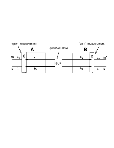
FIG. 2.: Experimental arrangement to test the Bell inequality for state (6), in the absence of loss. Our outcome at $A$ is designated $+1$ if $m\geq fN$, and $+1$ for $B$ if $m^{\prime}\geq fN$ , where $f$ is a preselected fraction. Predicted violations of the Bell inequality (5) are shown in Figure 3.

For the purpose of our particular experimental proposal we first demonstrate the failure of multi-particle local realism for the $N$-states (10) as follows. We choose the following binary classification of outcomes. If the result $m$ of the photon number measurement $c_{+}^{\dagger}c_{+}$ is greater than or equal to a certain fraction $f$ of the total photon number $m+k$ detected at $A$, then we have the result $+1$. Otherwise our result is $-1$. The outcome of a measurement at the location $B$ is classified as $+1$ or $-1$ in a similar manner.

A perfect correlation between $c_{+}^{\dagger}c_{+}$ and $d_{+}^{\dagger}d_{+}$ is predicted for the state (10) for $\theta=\phi$, a result $n$ for $c_{+}^{\dagger}c_{+}$ implying a result $n$ for $d_{+}^{\dagger}d_{+}$. For such situations of perfect correlation, we are able to deduce, if we assume local realism, following the reasoning of Einstein, Podolsky and Rosen${}^{\cite[cite]{[\@@bibref{Number}{EPR}{}{}]}}$, the existence of a set of “elements of reality”, $m_{\theta}^{A}$ and $m_{\phi}^{B}$, one for each subsystem at $A$ and $B$, and one for each choice of measurement angle, $\theta$ or $\phi$ at $A$ or $B$ respectively. The whole set of “elements of reality” ${m_{\theta}^{A}}$ and ${m_{\phi}^{B}}$ form a set of “hidden variables” representing the predetermined value of the results of “spin” measurements which can be attributed to the two particle system at a given time. This local realism assumption then implies the inequality (9).

The averages (9) can be calculated using quantum mechanics for the state (10) and the quantity $S$ computed. Violations of the Bell inequality (9) are found for a range of parameters as illustrated in Figure 3. Here we have selected the following relation between the angles: $\phi-\theta=\theta^{\prime}-\phi=\phi^{\prime}-\theta^{\prime}=\psi$ and $\phi^{\prime}-\theta=3\psi$. This combination has been shown to be optimal for the cases $N=1$${}^{\cite[cite]{[\@@bibref{Number}{Bell,CS}{}{}]}}$ and for all $N$ values with $f=1$${}^{\cite[cite]{[\@@bibref{Number}{Drum}{}{}]}}$. For each $f$, the value of $S$ tends to an asymptotic value as $N$ increases.

The violation of the Bell inequality (9) is greatest for $f=1$, where our result $+1$ at $A$, for example, corresponds to detecting all $N$ photons in the $c_{+}$ mode. This result has been presented previously${}^{\cite[cite]{[\@@bibref{Number}{Drum}{}{}]}}$. While this value of $f$ gives the strongest violation, the actual probability of the $+1$ event in this case becomes increasingly small as $N$ increases especially if detection inefficiencies are to be included as in later calculations. From this point of view, to look for the most feasible macroscopic experiment, the violations with reduced $f$ become important. We see that the magnitude of violation decreases with increasing $f$, so that the asymptotic value at $f=.5$ is 1.

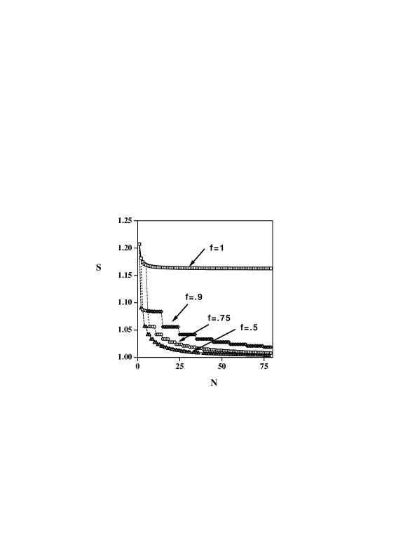
FIG. 3.: Plot of $S$ showing violation of the Bell inequality (5) (and (16)) versus $N$ for the quantum state (6). The results are optimised with respect to the angle $\psi$ as defined in the text. A violation is obtained when $S>1$. For $f=1$, the optimal angle $\psi$ is $.39,3.4,.22,.19,3.1$ for $N=1,2,3,4,80$ respectively. Results for values of $f=0.5-x$ are identical to those for $f=0.5+x$.

IV The effect of detection inefficiencies: derivation of a weaker Bell inequality

The effect of loss through detection inefficiency is important, since this limits the experimental feasibility of a test of the Bell inequality. To date to our knowledge the “strong” inequality of the type (9) has not yet been violated${}^{\cite[cite]{[\@@bibref{Number}{CS}{}{}]}}$ in any experiment involving photodetection, because of the detection inefficiencies which occur in photon counting experiments, although recent experiments by Rowe et al ${}^{\cite[cite]{[\@@bibref{Number}{exp}{}{}]}}$ violate a true Bell inequality for trapped ions, with limited spatial separation.

It is well documented${}^{\cite[cite]{[\@@bibref{Number}{Bell,CS}{}{}]}}$ that it is possible to derive, with the assumption of additional premises, a weaker form of the Bell- Clauser-Horne inequalities which have been violated in single photon counting experiments. Before proceeding to derive a “weak” Bell inequality for multi-particle detection, we outline the effect of detection inefficiencies on the violation, as shown in Figure 2, of the strong Bell inequality (9).

We introduce a transmission parameter $T$, defining $T$ as the probability that a single incoming photon will be detected, the intensity of the incoming field being reduced by the factor $T$. $T$ is directly related to the detector efficiency $\eta$ according to $T=\eta^{2}$. We model loss in the standard way by considering the measured field to be the transmitted output of a imaginary beam splitter with the input being the actual quantum field incident on the detector. The second input to the imaginary beam splitter is a vacuum field. Calculating the probabilities of this measured field is equivalent to using standard photocounting formulae which incorporate detection inefficiencies.

The following expression gives the final measured probability $P(m,k,m^{\prime},k^{\prime})$ for obtaining results $m,k,m^{\prime},k^{\prime}$ upon measurement of $c_{+}^{\dagger}c_{+}$, $c_{-}^{\dagger}c_{-}$ and $d_{+}^{\dagger}d_{+}$, $d_{-}^{\dagger}d_{-}$ respectively. Here $P_{Q}(m_{0},k_{0},m^{\prime}_{0},k^{\prime}_{0})$ is the quantum probability for obtaining $m_{0},k_{0},m^{\prime}_{0},k^{\prime}_{0}$ photons, upon measurement of $c_{+}^{\dagger}c_{+}$, $c_{-}^{\dagger}c_{-}$ and $d_{+}^{\dagger}d_{+}$, $d_{-}^{\dagger}d_{-}$, in the absence of detection losses. This quantum probability is derivable from (10).

$$P(m,k,m^{\prime},k^{\prime}) = T^{m+k+m^{\prime}+k^{\prime}}\sum_{r,q,s,t=0}^{\infty}(1-T)^{r+q+s+t}$$ (21)

$$\times C_{r}^{m+r}C_{q}^{k+q}C_{s}^{m^{\prime}+s}C_{t}^{k^{\prime}+t}$$ (22)

$$\times P_{Q}(m+r,k+q,m^{\prime}+s,k^{\prime}+t)$$ (23)

Here $C_{r}^{m+r}=(m+r)!/r!m!$, and $r,q,s,t$ represent the number of photons lost. We also consider the measured marginal probability.

$$P^{A}(m,k) = T^{m+k}\sum_{r,q=0}^{\infty}(1-T)^{r+q}C_{r}^{m+r}C_{q}^{k+q}$$ (24)

$$\times P_{Q}^{A}(m+r,k+q)$$ (25)

where $P_{Q}^{A}(m+r,k+q)$ represents the quantum probability for obtaining $m_{0},k_{0}$ photons upon measurement of $c_{+}^{\dagger}c_{+}$, $c_{-}^{\dagger}c_{-}$ in the absence of detection losses. This marginal quantum probability is derivable from (10).

With loss present there is a distinction between our actual quantum photon number $m_{0}$ present on the detectors, and the final readout photon number $m$, which is taken to be the result of the photon number measurement. (We must have $m\leq m_{0}$). Therefore a number of quantum probabilities will contribute in the calculation for the final measured probability. This complicating effect may be avoided in the following manner. The outcome at $A$ is labeled $+1$ only if $m\geq fN$ and $m+k=N$; and at $B$ if $m^{\prime}\geq fN$ and $m^{\prime}+k^{\prime}=N$. For $N$ photons detected at each location $A$ or $B$, we are restricted to the outcomes satisfying $m+k=m^{\prime}+k^{\prime}=N$ where loss has not occurred, for the given initial quantum state $|\varphi_{N}\rangle$. In this situation we get for the measured probabilities (23)

$$P(m,N-m,m^{\prime},N-m^{\prime})=$$ (26)

$$T^{2N}P_{Q}(m,N-m,m^{\prime},N-m^{\prime})$$ (27)

and for the marginal

$$P^{A}(m,N-m) = T^{N}P_{Q}^{A}(m,N-m)$$ (28)

Here $P_{Q}(m,N-m,m^{\prime},N-m^{\prime})$ is the quantum probability (in the absence of loss) that measurement of $c_{+}^{\dagger}c_{+}$ and $d_{+}^{\dagger}d_{+}$, for the state $|\varphi_{N}\rangle$ of equation (10), will give results $m$ and $m^{\prime}$ respectively. This quantum probability is calculated from the quantum amplitudes $C_{m,m^{\prime}}^{(N)}=\langle\varphi_{N}|m\rangle_{\theta}|m^{\prime}\rangle_{\phi}$, where $|m\rangle_{\theta}$, $|m^{\prime}\rangle_{\phi}$ are eigenstates of $c_{+}^{\dagger}c_{+}$, $d_{+}^{\dagger}d_{+}$ respectively, and is given by $P_{Q}(m,N-m,m^{\prime},N-m^{\prime})=|C_{m,m^{\prime}}^{(N)}|^{2}$ The quantum marginal for $|\varphi_{N}\rangle$ is $P_{Q}^{A}(m,N-m)=\sum_{m^{\prime}=0}^{N}|C_{m,m^{\prime}}^{(N)}|^{2}$.

The crucial effect of detection losses is that each measured joint probability contains the factor $T^{2N}$ where $2N$ is the total number of photons $m+k+m^{\prime}+k^{\prime}$ detected. This implies immediately extreme sensitivity of the multi-particle strong Bell inequality (9) to loss, since this inequality involves the marginal which scales as $T^{N}$. In the presence of loss $T$, the new predicted value for $S$ (required to test the strong Bell inequality (9)) is $T^{N}S_{0}$ where $S_{0}$ is the value “S” for $\varphi_{N}$ in the absence of loss as given graphically in Figure 3. It is seen then that we require $T$ to be $\sim(1/S_{0})^{1/N}$ or larger in order to obtain the violations of the no loop-hole inequalities (9). For $N=2$ $S_{0}=1.18$, and this requires at least $T>\sqrt{1/1.18}=.92$. This figure is at the limits of current technology, and compares with the requirement $T>.83$ for $N=1$.

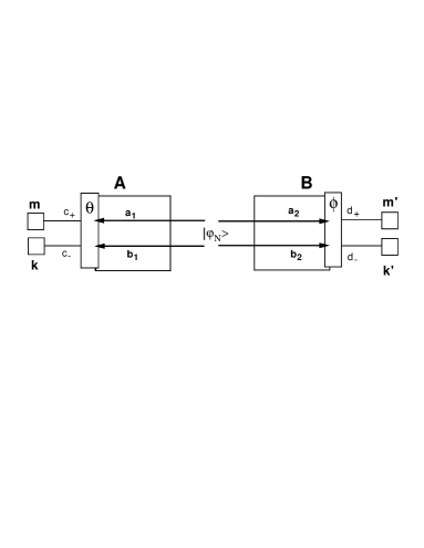
FIG. 4.: Schematic diagram of the experimental arrangement to test the Bell inequality for $|\varphi_{N}\rangle$ with detection inefficiencies present. Our outcome is $+1$ at $A$ if $m\geq fN$ and $m+k=N$; and $+1$ at $B$ if $m^{\prime}\geq fN$ and $m^{\prime}+k^{\prime}=N$. A violation of the no auxiliary-assumptions Bell inequality (5) is possible only for high detector efficiencies $T=\eta^{2}$. Predicted violations of the weak inequality (16) are as for Figure 3.

We now derive a multiparticle form of the weaker inequality so that we can also examine situations of significant detection loss. The result at $A$ is $+1$ if the number of photons $m$ detected at $c_{+}$ is $fN$ or more, and if the total number of photons $m+k$ detected at $A$ satisfies $m+k=N$; $p_{+}^{A}(\theta,\lambda)$ is the probability of this event given the hidden variable description $\lambda$. We define a new probability, $p_{+}^{A}(-,\lambda)$, that the total photon number $m+k$ (at location $A$) is $N$, given that the system is described by the hidden variables $\lambda$. This total probability is then assumed to be independent of the choice of polariser angle $\theta$ at $A$. Similarly we define a $p_{+}^{B}(-,\lambda)$, the probability that the total number of photons $m^{\prime}+k^{\prime}$ at $B$ is $N$. This total probability is then assumed to be independent of the polariser angle $\phi$ at $B$. We postulate as an additional premise that the hidden variable theories will satisfy

$$p_{+}^{A}(\theta,\lambda)\leq p_{+}^{A}(-,\lambda)$$ (29)

$$p_{+}^{B}(\phi,\lambda)\leq p_{+}^{B}(-,\lambda).$$ (30)

Using the procedure and theorems of the previous works of Clauser and Horne${}^{\cite[cite]{[\@@bibref{Number}{CS}{}{}]}}$ one may derive from the postulate of local realism and assumption (30) the following “weak” Clauser-Horne-Shimony-Holt Bell inequality, where the marginals are replaced by “one-sided” joint probabilities. Violation of this “weaker” Bell-CHSH inequality will only eliminate local hidden variable theories satisfying the auxiliary assumption. (30).

$$S_{W}=$$ (31)

$${\frac{{P_{++}^{AB}(\theta,\phi)-P_{++}^{AB}(\theta,\phi^{\prime})+P_{++}^{AB}(\theta^{\prime},\phi)+P_{++}^{AB}(\theta^{\prime},\phi^{\prime})}}{{P_{++}^{AB}(\theta^{\prime},-)+P_{++}^{AB}(-,\phi)}}}$$ (32)

$$\leq 1$$ (33)

Here we have defined new “one-sided” experimental joint probabilities as follows: $P_{++}^{AB}(\theta^{\prime},-)$, the joint probability of obtaining $+1$ at $A$, with the polariser at $A$ set at $\theta^{\prime}$, and of obtaining a total of $m^{\prime}+k^{\prime}=N$ photons at $B$. The joint probability $P_{++}^{AB}(-,\phi)$ is the probability of obtaining a total of $m+k=N$ photons at $A$, and of obtaining $+1$ at $B$, with the polariser at $B$ set at $\phi$.

For the situation where the detected probabilities are taken to be the quantum probabilities calculated directly from (10), so that we are ignoring additional losses and noise which may come from the detection and measurement process, we have the same result for the weak and strong inequalities (9) and (33).

Now to consider detection losses, we notice that the detrimental effect of the $T$ scaling apparent in (23) is removed by considering the weaker inequality, for which the marginal is replaced by the one-sided joint probability. The quantum predictions for the one-sided probabilities are for example

$$P_{++}^{AB}(\theta^{\prime},-) = \sum_{m\geq fN}^{N}\sum_{m^{\prime}=0}^{N}P(m,N-m,m^{\prime},N-m^{\prime})$$ (34)

$$= T^{2N}P_{Q}^{A}(m,N-m)$$ (35)

which we see from (27) is proportional to $T^{2N}$. Noting that $P_{Q}(m,N-m)$ is precisely the quantum marginal probability used in the strong inequality, we see that our predictions then for the violation of the weak inequality for the state (10) are as shown for the strong inequality in Figure 3 (meaning that the value for $S_{W}$ of equation (33) being given by the value of $S$ as shown in Figure 3).

V Proposed experiment to detect the violation of the multi-particle Bell inequality using parametric down conversion with and without entangled inputs

The prediction by quantum mechanics of the violation of a Bell inequality for the larger $N$ states (10) has not been tested experimentally. For this reason we investigate how one may achieve related violations of Bell inequalities using parametric down conversion. Previous work${}^{\cite[cite]{[\@@bibref{Number}{MB}{}{}]}}$ has shown how such violations are possible in the regime of low amplification, but this work was limited to situations of very low detection efficiencies.

We model the parametric down conversion by the Hamiltonian

$$H=i\hbar g\left(a_{1}^{\dagger}a_{2}^{\dagger}+b_{1}^{\dagger}b_{2}^{\dagger}\right)-i\hbar g\left(a_{1}a_{2}+b_{1}b_{2}\right)$$ (36)

Here we consider two parametric processes to make a four mode interaction${}^{\cite[cite]{[\@@bibref{Number}{4parexppro}{}{}]}}$, as may be achieved using two parametric amplifiers with Hamiltonians $H=i\hbar g(a_{1}^{\dagger}a_{2}^{\dagger}-a_{1}a_{2})$ and $H=i\hbar g(b_{1}^{\dagger}b_{2}^{\dagger}-b_{1}b_{2})$. The two outputs $a_{1},b_{1}$ are input to the polariser $\theta$ at $A$, while the two outputs $a_{2},b_{2}$ are input to the polariser $\phi$ at $B$. The time-dependent solution for the parametric process with vacuum inputs is

$$|\varphi\rangle=\sum_{N=0}^{\infty}c_{N}|\varphi_{N}\rangle$$ (37)

where $c_{N}=\sqrt{(N+1)}\Gamma^{N}/\widetilde{C}^{2}$  where $\widetilde{C}\equiv\cosh r$, $\widetilde{S}\equiv\sinh r$, $\Gamma\equiv\widetilde{S}\widetilde{/C}$ and “gain”: $r=gt$. The probability that a total of $N$ photons are detected at each location $A$ and $B$ is then $P(n)=|c_{N}|^{2}$ as plotted in Figure 5.

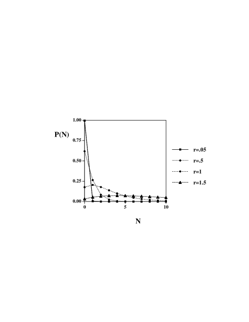
FIG. 5.: Plot of $P(N)=|c_{N}|^{2}$ the probability that a total of $N$ photons will be detected at each polariser location.

Of interest to us is the parametric output with the following polarization-entangled state as input.

$$|\varphi\rangle_{in}=\frac{1}{\sqrt{2}}\left(|1\rangle_{a_{1}}|1\rangle_{a_{2}}|0\rangle_{b_{1}}|0\rangle_{b_{2}}+|0\rangle_{a_{1}}|0\rangle_{a_{2}}|1\rangle_{b_{1}}|1\rangle_{b_{2}}\right)$$ (38)

This represents an example of the quantum injected optical parametric amplifier (QIOPA) realized experimentally by De Martini et al${}^{\cite[cite]{[\@@bibref{Number}{deM}{}{}]}}$. The active NL medium realizing the interaction (18) was a 2 mm BBO (beta-barium-borate) nonlinear crystal slab excited by a pulsed optical UV beam with wavelength $\lambda_{p}=345nm$. The duration of each UV excitation pulses was $150f\sec$ and the average UV power was $0.3W$. The UV beam was SHG generated by a mode-locked femtosecond Ti:Sa Laser (Coherent MIRA) optionally amplified by a high power Ti:Sa Regenerative Amplifier (Coherent REGA9000). The pulse repetition rate was $76.10^{6}Hz$ and $3.10^{5}Hz$ respectively in absence and in presence of the regenerative amplification. The maximum OPA “gain” obtained by the apparatus was: $r\approx 0.3$ and $r\approx 5.1$ respectively in absence and in presence of  the laser amplification. These figures lead respectively to the following values of the parameters: $\widetilde{C}=1.04$, $\Gamma=0.29$ and $\widetilde{C}=82$, $\Gamma\approx 1$. The typical quantum efficiency of the detectors was in the range: $\eta^{2}\approx 0.4-0.6$. The final output state generated by this apparatus is expressed by the multi-particle entangled state (37) but where $c_{N}=[\sqrt{(N+1)}\Gamma^{N}/\widetilde{C}^{2}]\times[(N-2\widetilde{S}^{2})/(\sqrt{2}\Gamma\widetilde{C}^{2})]$. The probability of an $n$ photon output at each location $A$ and $B$ is then given by $P(n)=|c_{n}|^{2}$ as is plotted in Figure 6, for various $r$.

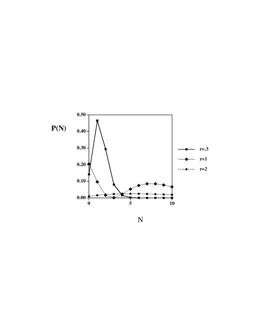
FIG. 6.: Plot of $P(N)=|c_{N}|^{2}$ the probability that a total of $N$ photons will be detected at each polariser location, for the entangled state input.

There are a number of approaches one can use to detect the quantum violation of the Bell inequalities. The particular method preferred will depend on the interaction strength $r$ and the degree of detection efficiency $\eta$.

FIG. 7.: Arrangement to test the Bell inequality for the parametric output. Our outcome is $+1$ at $A$ if $m=N$ and $m+k=N$; and $+1$ at $B$ if $m^{\prime}=N$ and $m^{\prime}+k^{\prime}=N$. We measure $P_{++}^{AB}(\theta,\phi)$ and, if testing the no loop-hole Bell inequality (5), the marginal probabilities $P_{+}^{A}(\theta)$ and $P_{+}^{B}(\phi)$. If testing the weaker Bell inequality (16), measurement is made of one-sided joint probabilities $P_{+}^{A}(\theta,-)$ and $P_{+}^{b}(-,\phi)$. A violation of the no auxiliary-assumptions Bell inequality is possible only for high $T=\eta^{2}$ (Figure 8). Predicted violations of a weak inequality (16) shown in Figure 9.

We propose here first the following experiment making use of the double-channeled polarisers (Figure 7) to detect the photon numbers of both orthogonal polarisations. This will allow the selection of a specified spin state $|\varphi_{N}\rangle$ and the observation of the violation predicted in Figure 3. Specifically we detect at locations $A$ and $B$ the photon numbers $c_{+}^{\dagger}c_{+}$, $c_{-}^{\dagger}c_{-}$, $d_{+}^{\dagger}d_{+}$ and $d_{-}^{\dagger}d_{-}$, where $c_{\pm}$ and $d_{\pm}$ are given by (4), and label the results $m$, $k$, $m^{\prime}$, and $k^{\prime}$ respectively. We designate the result of the measurement at $A$ to be $+1$ if our measured results $m$ and $k$ satisfy $m=N$ and also $m+k=N$. Otherwise our result is $-1$. Similarly we define the result at $B$ to be $+1$ if $m^{\prime}=N$ and $m^{\prime}+k^{\prime}=N$. By performing many such measurements over an ensemble, one can experimentally test the “strong” (no loop-hole) Bell inequality (9).

The calculation of $S$ as defined in (9) for the parametric amplifier state proceeds in straightforward manner. We define in general $P_{Q}(m,k,m^{\prime},k^{\prime})$ as the probability of detecting $m,k,m^{\prime},k^{\prime}$ photons upon measurements of $c_{+}^{\dagger}c_{+}$, $c_{-}^{\dagger}c_{-}$, $d_{+}^{\dagger}d_{+}$ and $d_{-}^{\dagger}d_{-}$ respectively, in the absence of loss. For $m+k=m^{\prime}+k^{\prime}=N$, we have

$$P_{Q}(m,N-m,m^{\prime},N-m^{\prime})=|c_{N}|^{2}|C_{m,m^{\prime}}^{(N)}|^{2}$$ (39)

$|c_{N}|^{2}$ is defined in (37), and $|C_{m,m^{\prime}}^{(N)}|^{2}$ is the probability that measurement of $c_{+}^{\dagger}c_{+}$ and $d_{+}^{\dagger}d_{+}$ for the state $|\varphi_{N}\rangle$ gives $m$ and $m^{\prime}$ respectively. Our required probabilities are then given as follows.

$$P_{++}^{AB}(\theta,\phi)=P_{Q}(N,0,N,0)=|c_{N}|^{2}|C_{N,N}^{(N)}|^{2}$$ (40)

and

$$P_{+}^{A}(\theta) = \sum_{m^{\prime}=0}^{\infty}P_{Q}(N,0,m^{\prime},N-m^{\prime})$$ (41)

$$= \sum_{m^{\prime}=0}^{\infty}|c_{N}|^{2}|C_{N,m^{\prime}}^{(N)}|^{2}$$ (42)

The detection of $m+k=N$ at $A$ is correlated with $m^{\prime}+k^{\prime}=N$ at $B$. Immediately then it is apparent that the factors $|c_{N}|^{2}$ in the joint and marginal probabilities in the final form of the Bell parameter $S$ for the strong inequality (9) will cancel. The predictions for the violation of (9), in the absence of loss, are as for the ideal spin state $|\varphi_{N}\rangle$. It is important to realize however that the actual probability of obtaining the event $+1$ is different in the parametric case, this probability being weighted by $|c_{N}|^{2}$, the probability of detecting $m+k=N$, that $N$ photons are incident on each polariser. While the joint probabilities are small, so is the true marginal, and we have a predicted violation of the strong Bell-Clauser-Horne inequality (9), without auxiliary assumptions.

The probabilities $P_{Q}(m,k,m^{\prime},k^{\prime})$ of (37) depend only on the angle difference $\phi-\theta$. We select the angle choice $\phi-\theta=\theta^{\prime}-\phi=\phi^{\prime}-\theta^{\prime}=\psi$ and $\phi^{\prime}-\theta=3\psi$ in line with previous work${}^{\cite[cite]{[\@@bibref{Number}{Drum,MB}{}{}]}}$ with the states $|\varphi_{N}\rangle$.

Our first objective would be to detect violations of the inequality for relatively low $N$, $N=2$ say. The choice of $r\sim 1$ gives the maximum probability of obtaining an event where $m+k=2$, although $r\sim.5$ would give a reasonable probability. For the optimal choice of angle $\psi$ (Figure 3) the probability of an actual event $+1$ for $N=2$ and $r\sim.5$ is $\sim.01$. For perfect detection efficiency the level of violation is given by $S=1.181$ as indicated in Figure 3.

We now need to consider the effect of detection inefficiencies. Our measured probabilities for obtaining $m,k,m^{\prime},k^{\prime}$ at each detector are given by (23) where now the quantum probabilities are calculated from (37). We note that with the restriction $m+k=m^{\prime}+k^{\prime}=N$, and $m=N$ we get

$$P(N,0,m^{\prime},N-m^{\prime})=T^{2N}\sum_{r,q,s,t=0}^{\infty}(1-T)^{r+q+s+t}$$ (43)

$$C_{r}^{N+r}C_{s}^{m^{\prime}+s}C_{t}^{N-m^{\prime}+t}P_{Q}(N+r,q,$$ (44)

$$\quad\quad\quad\quad\quad m^{\prime}+s,N-m^{\prime}+t)$$ (45)

where from (39) we have

$$P_{Q}(N+r,q,m^{\prime}+s,N-m^{\prime}+t)=$$ (46)

$$\delta(r+q-(s+t))|c_{N_{0}}|^{2}|C_{N+r,m^{\prime}+s}^{(N_{0}?)}|^{2}$$ (47)

where $N_{0}=N+r+q=N+s+t$. We note that for the quantum state (39) we require for nonzero probabilities $r+q=s+t$. The required joint probability $P_{++}^{AB}(\theta,\phi)$ becomes $P_{++}^{AB}(\theta,\phi)=P(N,0,N,0)$. The marginal probabilities needed for the strong Bell inequality (9) becomes for example $P_{+}^{A}(\theta)=P^{A}(N,0)$ where

$$P^{A}(N,0) = T^{N}\sum_{r,q=0}^{\infty}(1-T)^{r+q}C_{r}^{N+r}P_{Q}^{A}(N+r,q)$$ (48)

where

$$P_{Q}^{A}(N+r,q)=\sum_{m^{\prime}=0}^{\infty}|c_{N_{0}}|^{2}|C_{N+r,m^{\prime}}^{(N_{0}?)}|^{2}$$ (49)

where $N_{0}=N+r+q$.

Figure 8 reveals the effect on the violation of the strong Bell inequality, for various $r$, and for $N=2$. For the reasons discussed in the previous section, because the marginal probability scales as $T^{N}$ while the joint probabilities scale as $T^{2N}$, the violation is lost for small detection loss.

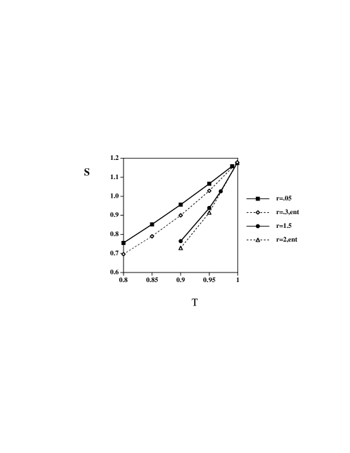
FIG. 8.: Effect, for various parametric coupling $r$, of detection inefficiencies on the violation of the strong Bell inequality (5), for the scheme described in Figure 7 with $N=2$. Here $T$ models detector losses, $T$ being the relative fraction of photons incident on each detector that are actually detected. The optimal angle $\psi$ for $N=2$ is $\sim 3.41$. The curves labeled “ent” represent predictions for the entangled input state.

To propose an experiment achievable with current detector efficiencies, we consider an appropriate weak Bell inequality. We define as before (Figure 7) the joint probability $P_{++}^{AB}(\theta,\phi)$ of obtaining $m=N$ and $m+k=N$ at $A$, and $m^{\prime}=N$ and $m^{\prime}+k^{\prime}=N$ at $B$. We define the joint one-sided probability $P_{++}^{AB}(\theta,-)$ of obtaining $m=N$ and $m+k=N$, and a total of $m^{\prime}+k^{\prime}=N$ photons at $B$. The one-sided probability $P_{++}^{AB}(-,\phi)$ is defined similarly. The auxiliary assumptions are made that for a hidden variable description $\lambda$, the probability $p_{+}^{A}(\theta,\lambda)$ of obtaining $m=N$ and $m+k=N$, and the probability $p_{+}^{A}(-,\lambda)$ of obtaining $m+k=N$ alone, satisfy

$$p_{+}^{A}(\theta,\lambda)\leq p_{+}^{A}(-,\lambda).$$ (50)

Also we assume $p_{+}^{A}(-,\lambda)$ is independent of $\theta$. Similar assumptions are made for $p_{+}^{B}(\phi,\lambda)$ and $p_{+}^{B}(-,\lambda)$. With these assumptions the weaker inequality (33) is derivable. The one-sided probability used in the test of the weak inequality (33) is given by $P_{++}^{AB}(\theta,-)=P^{AB}(N,0;-)$ where

$$P^{AB}(N,0;-) = \sum_{m^{\prime}=0}^{N}P(N,0,m^{\prime},N-m^{\prime})$$ (51)

With a total of $N$ photons detected at both locations $A$ and $B$, we ensure all probabilities scale as $T^{2N}$.

The existence of the higher spin states $|\varphi_{M}\rangle$ where $M>N$ in the parametric output means that detector inefficiencies alter the violation of even the weak Bell inequality. Figure 9 illustrates the effect of detection inefficiencies on the violation of the weak inequalities (33), the effect being more significant for higher $r$ values where the states $|\varphi_{M}\rangle$, where $M>N$, contribute more significantly. Smaller $r$ values suffer the disadvantage however that the probability of an actual event $+1$ becomes small due to the small probability of $N=2$ photons actually being incident on the polariser. The sensitivity of the violations to loss is not so great that the experiment would be impossible for $r\sim.5$.

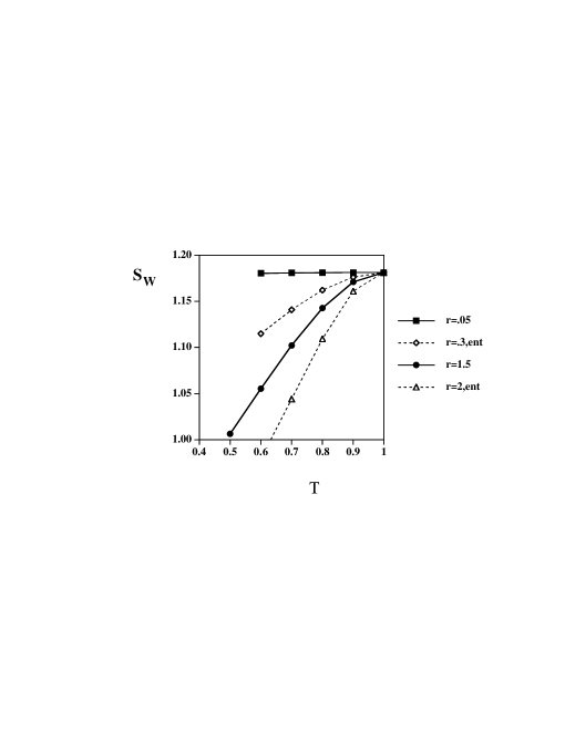
FIG. 9.: Effect of detection inefficiencies on the violation of the weak Bell inequality (16), for the scheme described in figure 7 where $N=2$. Here $T$ represents detector losses, $T$ being the relative fraction of incident photons actually detected. The optimal angle $\psi$ for $N=2$ is $\sim 3.41$. The curves labeled “ent” are predictions for the entangled input state.

A point to be made concerns the alternative situation of a one-channeled polariser where only the photon number $m$ and $m^{\prime}$ can be detected. Here the prediction is different due to the contribution of the $N+1$ spin state which can contribute an $m=N$ event (with $k=1$) potentially decreasing the violation of the inequality.

VI Proposed experiment to detect the violation of the Bell inequality using high flux parametric down conversion

As one increases the output intensities of the parametric device, the actual probability of detecting $N$ photons transmitted through our polariser decreases, in other words the probability of detecting the event $+1$, described in the last section, becomes smaller. To combat this we propose in this section that our outcome be a range of photon number values. Here we are interested in the regime of high amplification${}^{\cite[cite]{[\@@bibref{Number}{Smithey}{}{}]}}$ where the output fluxes of signal and idler are high, and where one can use highly efficient photodiode detectors.

We now propose the following experiment. We detect at locations $A$ and $B$ the photon numbers $c_{+}^{\dagger}c_{+}$, $c_{-}^{\dagger}c_{-}$, $d_{+}^{\dagger}d_{+}$ and $d_{-}^{\dagger}d_{-}$, where $c_{\pm}$ and $d_{\pm}$ are given by (3). The mean photon number incident on each polariser is $xm=<c_{+}^{\dagger}c_{+}>+<c_{-}^{\dagger}c_{-}>=<d_{+}^{\dagger}d_{+}>+<d_{-}^{\dagger}d_{-}>$ where $xm=2sinh^{2}(r)$. We denote the result for $c_{+}^{\dagger}c_{+}$ and $c_{-}^{\dagger}c_{-}$ at $A$ by $m$ and $k$ respectively, and the results of $d_{+}^{\dagger}d_{+}$ and $d_{-}^{\dagger}d_{-}$ at $B$ by $m^{\prime}$ and $k^{\prime}$ respectively (Figure 7). We define $XM$ to be the integer nearest in value to the mean $xm$. We designate the result of the measurement at $A$ to be $+1$ if our measured results $m$ and $k$ satisfy $m\geq XM$ and also $XM\leq m+k\leq XM+\Delta$. Otherwise our result is $-1$. Similarly we define the result at $B$ to be $+1$ if $m^{\prime}\geq XM$ and $XM\leq m^{\prime}+k^{\prime}\leq XM+\Delta$.

By performing many such measurements over an ensemble, one can experimentally determine the following: $P_{++}^{AB}\left(\theta,\phi\right)$ the probability of obtaining $+1$ at $A$ and $+1$ at $B$ upon simultaneous measurement with $\theta$ at $A$ and $\phi$ at $B$; $P_{+}^{A}\left(\theta\right)$ the marginal probability for obtaining the result $+1$ upon measurement with $\theta$ at $A$; and $P_{+}^{B}\left(\phi\right)$ the marginal probability of obtaining the result $+1$ upon measurement with $\phi$ at $B$.

Local hidden variables will predict as discussed in section 2 the strong Bell inequality (9). We define $P(m,k,m^{\prime},k^{\prime})$ as the probability of detecting $m,k,m^{\prime}$and $k^{\prime}$ photons for measurements of $c_{+}^{\dagger}c_{+}$, $c_{-}^{\dagger}c_{-}$, $d_{+}^{\dagger}d_{+}$ and $d_{-}^{\dagger}d_{-}$ respectively. The probability of results $m$ and $k$ upon measurement of $c_{+}^{\dagger}c_{+}$and $c_{-}^{\dagger}c_{-}$ is defined as $P^{A}(m,k)$. We have in the absence of loss, where $m+k=m^{\prime}+k^{\prime}=N$ is ensured,

$$P(m,N-m,m^{\prime},N-m^{\prime}) = |c_{N}|^{2}|C_{m,m^{\prime}}^{(N)}|^{2}$$ (52)

$$P^{A}(m,N-m) = \sum_{m^{\prime}=0}^{N}|c_{N}|^{2}|C_{m,m^{\prime}}^{(N)}|^{2}$$ (53)

where all other probabilities are zero. Here $|c_{N}|^{2}$ is defined in (37), and $|C_{m,m^{\prime}}^{(N)}|^{2}$ is the probability that measurement of $c_{+}^{\dagger}c_{+}$ and $d_{+}^{\dagger}d_{+}$ for the state $|\varphi_{N}\rangle$ gives $m$ and $m^{\prime}$ respectively, with no loss. The probability $P(m,m^{\prime})$ of getting $m$ and $m^{\prime}$ for $c_{+}^{\dagger}c_{+}$ and $d_{+}^{\dagger}d_{+}$ respectively, while the total $m+k$ is restricted to $XM\leq m+k\leq XM+\Delta$, and $m+k=m^{\prime}+k^{\prime}$ is restricted to $XM\leq m^{\prime}+k^{\prime}\leq XM+\Delta$, is given generally as

$$P^{AB}(m,m^{\prime})=\sum_{k=XM-m}^{XM+\Delta-m}\sum_{k^{\prime}=XM-m^{\prime}}^{XM+\Delta-m^{\prime}}P(m,k,m^{\prime},k^{\prime})$$ (54)

The corresponding marginal probability is

$$P^{A}(m)=\sum_{k=XM-m}^{XM+\Delta-m}P^{A}(m,k)$$ (55)

Our required probabilities are then given as follows

$$P_{++}^{AB}(\theta,\phi)=\sum_{m,m^{\prime}=XM}^{XM+\Delta}P^{AB}(m,m^{\prime})$$ (56)

and for the marginal

$$P_{+}^{A}(\theta)=\sum_{m=XM}^{XM+\Delta}P^{A}(m)$$ (57)

For the purpose of a weaker Bell inequality we also define a one-sided probability

$$P_{++}^{AB}(\theta,-)=\sum_{m=XM}^{XM+\Delta}\sum_{m^{\prime}=0}^{XM+\Delta}P^{AB}(m,m^{\prime})$$ (58)

The probabilities $P(m,k,m^{\prime},k^{\prime})$ depend only on the angle difference $\phi-\theta$. We select the angle choice $\phi-\theta=\theta^{\prime}-\phi=\phi^{\prime}-\theta^{\prime}=\psi$ and $\phi^{\prime}-\theta=3\psi$ in line with previous work${}^{\cite[cite]{[\@@bibref{Number}{Bell,Drum}{}{}]}}$ with the states $|\varphi_{N}\rangle$.

Results for $S$, optimizing $\psi$ to give maximum $S$, are presented in the Figure 9. With the choice $\Delta=0$, we will get only one of the $|\varphi_{N}\rangle$ contributing. The results for $S$ will be identical${}^{\cite[cite]{[\@@bibref{Number}{Drum}{}{}]}}$ to that obtained for the $|\varphi_{XM}\rangle$ state, where a clear violation of the Bell inequality (9) is obtained even for very large $N=XM$. The difficulty with such a situation however is that in the regime of higher $r$ where greater signal intensities are generated the probability that the total number $m+k$ of photons $c_{+}^{\dagger}c_{+}+c_{-}^{\dagger}c_{-}$ is just this fixed number is very small, making the probability of our $+1$ outcome tiny. We are more interested in situations where the intensity on the detectors is large but also where the probability that $XM\leq m+k\leq XM+\Delta$ is significant. This is achieved by increasing the range $\Delta$. Violations of the Bell inequality are still possible ($S\geq 1$) but the degree of violation is reduced, the limiting value for large $\Delta$ approaching $1$ as $XM$ increases.

FIG. 10.: Plot of violation of the strong Bell inequality where we designate the result of the measurement at $A$ to be $+1$ if our measured results $m$ and $k$ satisfy $m\geq XM$ and also $XM-\Delta\leq m+k\leq XM+\Delta$. Otherwise our result is $-1$. Similarly we define the result at $B$ to be $+1$ if $m^{\prime}\geq XM$ and $XM\leq m^{\prime}+k^{\prime}\leq XM+\Delta$. For $r=1.65$ we have $XM=13$ and for $r=1.95$, $XM=24$.

FIG. 11.: Plot of the effect of detection losses on the violation of the no loop-hole Bell inequality test (5) as explained in figure 10 above. Here $r=1.65$ we have $XM=13$.

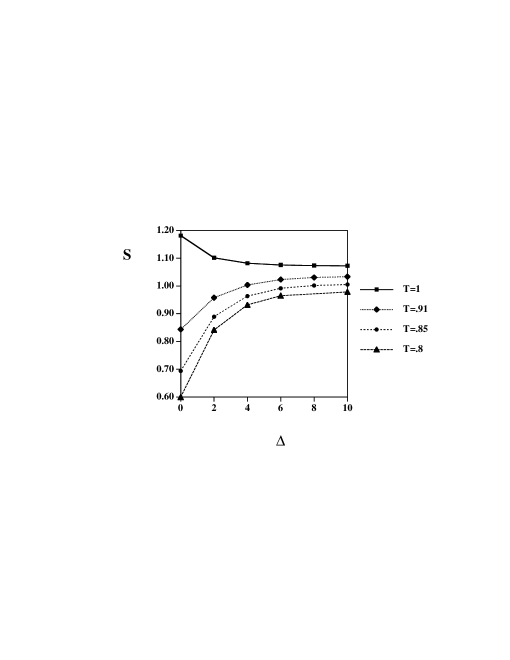
FIG. 12.: Plot of the effect of detection losses on the violation of the no loop-hole Bell inequality test (5) as explained in figure 10 above. Here $r=0.9$ we have $XM=2$.

The sensitivity to loss can be evaluated by calculating in (54) (and in the equations for the marginal probabilities such as $P^{A}(m)$) the measured probabilities $P(m,k,m^{\prime},k^{\prime})$ and $P^{A}(m,k)$ as given by (23) and (25). The effect on the violation of the no loop-hole Bell inequality (9) is given in Figures 11 and 12. Sensitivity is strong for low $\Delta$ but decreases as the range $\Delta$ increases. This provides a potential opportunity to test a strong no-auxiliary multi-particle Bell inequality for lower detector inefficiencies than indicated by the $\Delta=0$ regime discussed in the previous section.

VII Conclusions

We have presented a proposal to test the predictions of quantum mechanics against those of local hidden variable theories for multi-particle entangled states generated using parametric down conversion, where measurement is made on systems of more than one particle. A calculation is given of the detector efficiencies required to test directly the “no loop-hole”multi-particle Bell inequality. In view of the limitation of current detector efficiencies, it is necessary to consider initially tests of a “weaker” Bell inequality derived with additional auxiliary assumptions, and to therefore extend previous such derivations to the multi-particle situation we consider here.

VIII
Acknowledgments

F.D.M. acknowledges the Italian Ministero dell’Universita’ e della Ricerca Scientifica e Tecnologica (MURST) and the FET European Network IST-2000-29681(ATESIT) on “Quantum Information

”, for funding.

REFERENCES

- [1] A. Einstein, B. Podolsky and N. Rosen, Phys. Rev. 47, 777, (1935).
- [2] D. Bohm, “Quantum Theory” (Prentice-Hall, Englewood Cliffs, NJ, 1951).
- [3] J. S. Bell, Physics, 1, 195, (19965). J. S. Bell, “Speakable and Unspeakable in Quantum Mechanics” (Cambridge Univ. Press, Cambridge, 1988). J. S. Bell, Physics 1, 195 (1964).
- [4] J. F. Clauser and A. Shimony, Rep. Prog. Phys. 41, 1881 (1978), and references therein. J. F. Clauser, M. A. Horne, A. Shimony, and R. A. Holt, Phys. Rev. Lett. 23, 880 (1969).
- [5] D. M. Greenberger, M. A. Horne, A. Shimony and A. Zeilinger, Am. J. Phys. 58, 1131 (1990).
- [6] A. Aspect, P. Grangier and G. Roger, Phys. Rev. Lett. 49, 91, (1982). A. Aspect, J. Dalibard and G. Roger, ibid. 49, 1804, (1982). Y. H. Shih and C. O. Alley, Phys. Rev. Lett. 61, 2921, (1988). Z. Y. Ou and L. Mandel, Phys. Rev. Lett. 61, 50, (1988). J. G. Rarity and P. R. Tapster, Phys. Rev. Lett. 64, 2495, (1990). J. Brendel, E. Mohler and W. Martienssen, Europhys. Lett. 20, 575, (1992). P. G. Kwiat, A. M. Steinberg and R. Y. Chiao, Phys. Rev. A 47, 2472, (1993). T. E. Kiess, Y. H. Shih, A. V. Sergienko and C. O. Alley, Phys. Rev. Lett. 71 3893, (1993). P. G. Kwiat, K. Mattle, H. Weinfurter, A. Zeilinger, A. V. Sergienko and Y. Shih, Phys. Rev. Lett. 75, 4337, (1995), D. V. Strekalov, T. B. Pittman, A. V. Sergienko, Y. H. Shih and P. G. Kwiat, Phys. Rev. A 54, 1, (1996). W. Gregor, T. Jennewein and A. Zeilinger, Phys. Rev. Lett. 81, 5039 (1998). A. Zeilinger, Rev. Mod. Phys. 71, 5288, (1998). M.A. Rowe, D. Kielpinski,V. Meyer, C. A. Sackett, W. M. Itano, C. Monroe, D. J. Wineland, Nature 409, 791 (2001).
- [7] C. A. Sackett, D. Kielpinski, B. E. King, C. Langer, V. Meyer, C. J. Myatt, M. Rowe, Q. A. Turchette, W. M. Itano, D. J. Wineland, C. Monroe, Nature 404, 256 (2000).
- [8] A. Rauschenbeutel, G. Nogues, S. Osnaghi, P. Bertet, M. Brune, J. Raimond and S. Haroche, Science 288, 2024 (2000).
- [9] J. W. Pan, D. Bouwmeester, M. Daniell, H. Weinfurter, A. Zeilinger, Nature 403, 515 (2000).
- [10] Z. Y. Ou, S. F. Pereira, H. J. Kimble and K. C. Peng, Phys. Rev. Lett. 68, 3663 (1992).
- [11] Yun Zhang, Hai Wang, Xiaoying Li,Jietai Jing, Changde Xie and Kunchi Peng, Phys. Rev. A 62, 023813 (2000).
- [12] Ch. Silberhorn, P. K. Lam, O. Weiss, F. Koenig, N. Korolkova and G. Leuchs, presented at Europe IQEC (2000), quant-ph/0103002.
- [13] M. D. Reid, Europhys. Lett. 36, 1 (1996); Quantum Semiclass. Opt. 9, 489 (1997); M. D. Reid and P. Deuar, Ann. Phys. 265, 52 (1998); M. D. Reid, Phys. Rev. A. 62 022110 (2000); quant-ph/0101050
- [14] V. Giovannetti, S. Mancini and P. Tombesi, quant-ph/0005066.
- [15] N. D. Mermin, Phys. Rev. D 22, 356 (1980) . A. Garg and N. D. Mermin, Phys. Rev. Lett. 49, 901, 1294 (1982).
- [16] N. D. Mermin and G. M. Schwarz, Found. Phys. 12, 101 (1982).
- [17] P. D. Drummond, Phys. Rev. Lett. 50, 1407 (1983).
- [18] A. Peres, Found. Phys. 22,1819 (1992). A. Peres, “Quantum Theory: Concepts and Methods”, (Kluwer academic, Dordrecht, 1993).
- [19] A. Garg and N. D. Mermin, Phys. Rev. Lett. 49, 901 (1982); Phys. Rev. D 27, 339 (1983). N. D. Mermin, Phys. Rev. Lett. 65, 1838 (1990). S. M. Roy and V. Singh, Phys. Rev. Lett. 67 , 2761 (1991). A. Peres, Phys. Rev. A 46, 4413 (1992). A. Peres, Found. Phys. 22,1819 (1992). M. D. Reid and W. J. Munro, Phys. Rev. Lett. 69, 997 (1992). B. C. Sanders, Phys. Rev. A 45, 6811 (1992). G. S. Agarwal, Phys. Rev. A 47, 4608 (1993). D. Home and A. S. Majumdar, Phys. Rev. A 52, 4959 (1995). C. Gerry, Phys. Rev. A 54, 2529, (1996). A. Beige, W. J. Munro and P. L. Knight, Phys. Rev. A62, 052102 (2000).
- [20] K. Banaszek and K. Wodkiewicz, Phys. Rev. A 58, 4345 (1998); Phys. Rev. Lett. 82, 2009 (1999).
- [21] W. J. Munro and M. D. Reid, Phys. Rev. A 47, 4412 (1993).
- [22] J. G. Rarity and P. R. Tapster, Phys. Rev. Lett. A 64, 2495 (1990). M. A. Horne, A. Shimony and A. Zeilinger, Phys. Rev. Lett. 62, 2209 (1989). M. D. Reid and D. F. Walls, Phys. Rev. A 34, 1260 (1985). . P. G. Kwiat, K. Mattle, H. Weinfurter, A. Zeilinger, A. V. Sergienko and Y. Shih, Phys. Rev. Lett. 75, 4337, (1995). M. Marte, Phys. Rev. Lett. 74, 4815 (1995).
- [23] F. De Martini, Phys. Rev. Lett. 81, 2842 (1998); F. De Martini, V.Mussi and F. Bovino, Optics Comm.179, 581 (2000), F. De Martini and G. Di Giuseppe, quant-phys/0011081 and submitted to Phys. Rev. Lett.
- [24] D. T. Smithey, M. Beck, M. Belsley, and M. G. Raymer, Phys. Rev. Lett. 69, 2650 (1992).