Propagation of Raman-matched laser pulses through a Bose-Einstein condensate

Abstract

We investigate the role of non-uniform spatial density profiles of trapped atomic Bose-Einstein condensates in the propagation of Raman-matched laser pulses under conditions for electromagnetically induced transparency (EIT). We find that the sharp edged axial density profile of an interacting condensate (due to a balance between external trap and repulsive atomic interaction) is advantageous for obtaining ultra slow averaged group velocities. Our results are in good quantitative agreement with a recent experiment report [Nature 397, 594 (1999)].

1 Introduction

Recent reports [1, 2] of stopping a near resonant laser pulse inside highly absorptive atomic vapors has attracted tremendous public interests. Physically, this magic like ‘light trapping’ is due to delicate quantum interference under the condition of electromagnetically induced transparency (EIT) [3, 4, 5]. In these experiments, a dynamical controlled pump field effects the conversion of a Raman-matched probe field into atomic Raman coherence of the medium. Broadly interpreted, it provides a mechanism for storage of quantum information encoded in the probe field. The experimenters also demonstrated the read-out by back-converting stored atomic Raman coherence into a new light field. EIT typically occurs under conditions of complete opaqueness which prevents the propagation of incoherent light; while a coherent propagation can succeed because of interference induced cancellation of one-path absorption. In several earlier experiments, ultra slow light propagation was observed in Bose-Einstein condensate (BEC) of Na atoms [$\sim 17$ (m/s)[6] and $\sim 1$ (m/s)[7]], in hot rubidium vapor [$\sim 90$ m/s [8] and $\sim 8$ m/s [9]], and in a Pr:YSO crystal [$\sim 45$ m/s [10]]. As the net reduction of light speed is about the same order of magnitude in different host media, one may argue that being bose condensed is perhaps not so crucial. From a practical point of view, however, the long coherence time of BEC does prove to be advantageous. Compared with a homogeneous media [2, 8, 9, 10], using a trapped atomic BEC as the EIT medium raises an important complication from its spatially inhomogeneous density profile (due to both external trapping and atom-atom interaction) [1, 6, 7]. A consistent interpretation therefore requires careful spatial averaging and theoretical modeling. In this article we elucidate the effect of such a spatial average which also takes into account atom-atom interaction.

Slow light propagation can be phenomenologically understood in terms of a high index of refraction (slow phase velocity) or a high dispersion-like feature (slow group velocity). It has been extensively studied for atomic media exhibit EIT [3]. Under typical conditions, such media are highly sought-after as there exist many potential technological applications, e.g. optical delay lines [6], quantum entanglement of slow photons [12], non-classical (e.g. squeezed) and entangled atomic ensembles [13], and quantum memories [1, 2, 5]. Other potential fundamental applications include: high nonlinear coupling between weak fields [6, 11], quantum non-demolishing measurements and high precision spectroscopy [14], and as narrow-band sources for non-classical radiation [15]. In addition to a complete stoppage of light [5], possibilities of even negative group velocities have been discussed [16]. We expect our investigation will shed light onto the realization of these applications in addition to providing a satisfactory understanding of slow light propagation in trapped atomic BEC.

The paper is organized as follows: In Sec. II we briefly review our formulation of near-resonant light propagation in dispersive medium. Section III is devoted to the discussion of laser pulse propagation under conditions of EIT from a pair of Raman-matched pulses. In Sec. IV we discuss the widely used two-component model for the density profile of a trapped interacting BEC. In Sec. V we present numerical studies and compare them with the earlier experimental report of Hau et al. [6]. Finally we conclude in Sec. VI.

2 Group velocity in a dispersive media

Propagation of light in a non-magnetic, charge-free, dispersive medium is governed by the second order wave equation

$$\nabla^{2}_{T}\vec{E}(\vec{r},t)+\frac{\partial^{2}\vec{E}(\vec{r},t)}{\partial z^{2}}-\frac{1}{c^{2}}\frac{\partial^{2}\vec{E}(\vec{r},t)}{\partial t^{2}}+\vec{\nabla}\left(\vec{\nabla}\cdot\vec{P}(\vec{r},t)\right)=\frac{4\pi}{c^{2}}\frac{\partial^{2}\vec{P}(\vec{r},t)}{\partial t^{2}},$$ (1)

where $\vec{E}$ is the coarse grained electric field of the propagating light and $\vec{P}$ is the induced macroscopic medium polarization. Limiting our discussion to a medium where spatial changes of the dielectric function are negligible within a wavelength of propagating light, the last term in the lhs of Eq. (1) can be neglected. Although this is a standard approximation, we cautiously point out that it may lead to significant errors near the boundary of an interacting atomic BEC, where the gas density profile changes rapidly [17]. In our numerical simulation we also neglected this term based on an additional argument. For a transverse field propagating along z-axis, the coupling of $\vec{\nabla}\cdot\vec{P}(\vec{r},t)$ is mainly along the orthogonal direction from the propagation direction. Therefore we only expect slight modifications to field distribution in the immediate neighborhood of the BEC boundary. We reconstruct the behavior of injected pulse in this region from an interpolation between its behaviors in and out of the condensate. The propagation is always started away from the edge of the BEC and the thermal component density contribution of trapped atomic gas in fully included. In the paraxial approximation limit, we make further simplification of Eq. (1) by neglecting the transverse Laplacian $\nabla_{T}^{2}\vec{E}(\vec{r},t)$. This latter approximation is checked for self-consistency in comparison with experiments performed with a trapped BEC.

We consider the propagation of a light pulse with central wave vector $\vec{k}_{0}$ along the propagation ($z$) axis and carrier frequency $\omega_{0}$. In a dispersive medium, characterized by a complex refractive index $n(k,\omega)$ at frequency $\omega$ and wave number $k$, the relation between the carrier frequency and wavevector is the dispersion relation $n(k_{0},\omega_{0})\omega_{0}=ck_{0}$. Typically $n(k_{0},\omega_{0})\approx 1$ at resonance, therefore $\omega_{0}=ck_{0}$ remains approximately valid throughout such a medium for near-resonant carrier frequencies. Employing the slowly varying phase and amplitude approximation for the complex amplitudes $\{{\cal P},{\cal E}\}$, defined by $\{P,E\}=\Re[\{{\cal P},{\cal E}\}\exp{(ik_{0}z-i\omega_{0}t)}]$, we obtain

$$\frac{\partial{\cal E}}{\partial z}+\frac{1}{c}\frac{\partial{\cal E}}{\partial t}=-\frac{4\pi}{c}\frac{\partial{\cal P}}{\partial t}+2\pi ik_{0}{\cal P}.$$ (2)

The medium polarization is to be calculated from the linear response of atoms to the weak probe field $E$. It is customarily described in terms of an electric susceptibility $\chi(\vec{r},t)$ according to

$${\cal P}(z,t)=\int\,dz^{\prime}\int\,dt^{\prime}\chi(z-z^{\prime},t-t^{\prime}){\cal E}(z^{\prime},t^{\prime}).$$ (3)

All macroscopic physical quantities used are assumed to be derived from a coarse graining procedure where the medium is assumed isotropic microscopically. According to the convolution theorem, the integral in the rhs of Eq. (3) can be expressed as,

$${\cal P}(z,t)=\int\,d\omega\int\,dk\,\chi(k,\omega){\cal E}(k,\omega)e^{ikz-i\omega t},$$ (4)

which is equivalent to ${\cal P}(k,\omega)=\chi(k,\omega){\cal E}(k,\omega)$. To simplify the notation, we will reference $(k,\omega)$ with respect to the origin $(k_{0},\omega_{0})$. Expanding $\chi(k,\omega)$ to first order around $\chi_{0}=\chi(k_{0},\omega_{0})$ one obtains [18]

$${\cal P}(z,t)=\chi(0){\cal E}(z,t)+i\left(\frac{\partial\chi}{\partial\omega}\right)_{0}\frac{\partial{\cal E}}{\partial t}-i\left(\frac{\partial\chi}{\partial k}\right)_{0}\frac{\partial{\cal E}}{\partial z},$$ (5)

which upon substituting into Eq. (2) yields [8, 16]

$$\left[1-2\pi k_{0}\left(\frac{\partial\chi}{\partial k}\right)_{0}\right]\frac{\partial{\cal E}}{\partial z}+$$ (6)

$$+ \frac{1}{c}\left[1+2\pi\chi(0)+2\pi\omega_{0}\left(\frac{\partial\chi}{\partial\omega}\right)_{0}\right]\frac{\partial{\cal E}}{\partial t}=2\pi ik_{0}\chi(0){\cal E}.$$

Under the assumption of slow spatial variations we can neglect the spatial dispersion term $k_{0}(\partial\chi/\partial k)_{0}$. We now introduce a complex valued function $N_{g}=1+2\pi\chi(0)+2\pi\omega_{0}\partial\chi/\partial\omega_{0}$, whose real (imaginary) part will be called group index (phase correlation index). The real (imaginary) part of $1+2\pi\chi(0)$ will be called refractive (loss or gain) index. Unless otherwise stated, we use $(.)^{\prime}$ and $(.)^{\prime\prime}$ to denote real and imaginary part of (.) throughout this article. The Wave equation (6) then simplifies to

$$\frac{\partial{\cal E}}{\partial z}+\frac{1}{v_{g}}\frac{\partial{\cal E}}{\partial t}=\alpha{\cal E},$$ (7)

where the complex parameter $\alpha=2\pi ik_{0}\chi(0)$ mainly governs pulse attenuation or amplification while the complex velocity function $v_{g}=c/N_{g}$ is mostly responsible for the propagation. In order to appreciate the kinematic meaning of $v_{g}$, it is helpful to cast the complex wave equation (7) into two coupled equations for real functions $\phi$ (phase) and $U$ (amplitude) defined according to ${\cal E}=Ue^{i\phi}$,

$$\frac{\partial U}{\partial z}+\frac{N_{g}^{\prime}}{c}\frac{\partial U}{\partial t} = -2\pi k_{0}\chi^{\prime\prime}(0)U+\frac{N_{g}^{\prime\prime}}{c}U\frac{\partial\phi}{\partial t},$$ (8)

$$\frac{\partial\phi}{\partial z}+\frac{N_{g}^{\prime}}{c}\frac{\partial\phi}{\partial t} = 2\pi k_{0}\chi^{\prime}(0)-\frac{N_{g}^{\prime\prime}}{c}\frac{\partial\ln{U}}{\partial t}.$$ (9)

The propagation of a signal as well as the signal speed can only be defined for such real observables. When $N_{g}^{\prime\prime}\approx 0$, these two equations become uncoupled with Eq. (8) governing pulse propagation kinematics. Consequently $v_{g}=c/N_{g}^{\prime}$ can be defined as group velocity. Ambiguity arises when Eqs. (8) and (9) are coupled for $N_{g}^{\prime\prime}\neq 0$. Our choice of group velocity definition $v_{g}$ is equivalent to $v_{g}=c/\Re(N_{g})$, which is not the same as $v_{g}=\Re(d\omega/dk)=\Re(c/N_{g})$[16]. When $N_{g}^{\prime\prime}$ is not negligible these two definitions generally lead to different results as can be exemplified by selected results presented in Figs. 1 and 2, which compares calculated group velocities according to the above two different definitions.

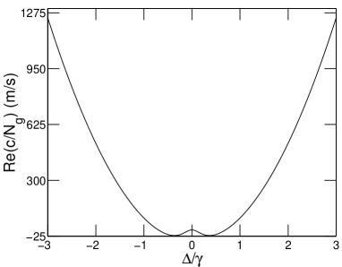
Figure 1: The group velocity for a pulse propagating through a three-level Raman EIT medium of a uniform density calculated according to $v_{g}=\Re(c/N_{g})$. See later for the discussion gas density $\sim 3.3\times 10^{12}({\rm cm}^{-3})$, $\lambda_{0}=589$(nm), $\Gamma_{31}=0.5\gamma$, $\Gamma_{21}=(2\pi)10^{3}$ (Hz), $\Omega=0.56\gamma$, and $\gamma=(2\pi)10.01$ (MHz).

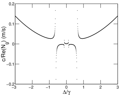
Figure 2: Same as in Fig. 1 except we used $v_{g}=c/\Re(N_{g})$.

The calculation of $N_{g}$ as well as the details of our model will be given in the next section. At zero probe field detuning $N_{g}^{\prime\prime}$ vanishes and the above two definitions become identical. For detunings where $N_{g}^{\prime}$ vanishes, however, the two results are drastically different as such points are singularities for $v_{g}=c/N_{g}^{\prime}$. Thus, it seems more appropriate to treat the group velocity as a complex function in general, and assign a real physical meaning operationally based on the pulse delays. The imaginary part $N_{g}^{{}^{\prime\prime}}$ causes non-trivial coupling between the amplitude and phase of a propagating pulse. As a result of this coupling, different propagation and transmission characteristics can occur. This situation is similar to the description of quantum tunneling in terms of a complex time and velocity [19]. When $N_{g}^{\prime\prime}$ is large, the amplitude and phase equations are strongly coupled, resulting in strong phase-amplitude correlations. This equation set can also be compared to the semi-classical laser equation [4] where similar situations arise. One important consequence of such amplitude-phase correlations is a ‘false’ gain phenomenon, or a perceived superluminal propagation [20]. To illustrate such effects explicitly, we consider a gas medium of uniform density. In this case, Eq. (7) can be solved with an ansatz $\exp{[\alpha(z-z_{0})]}f[t-(z-z_{0})/v]$, where $z_{0}$ is the injection location of the incoming pulse and $f(.)$ is an arbitrary complex valued function at the complex retarded time due to complex velocity $v=C/(N_{g}^{\prime}+iN_{g}^{\prime\prime})$. Assuming a Gaussian temporal profile for the injected pulse at $z_{0}$ as $\exp{(-at^{2})}$, the phase and amplitude functions $U$ and $\phi$ can be solved

$$U(z,t) = \exp{\left\{\alpha^{\prime}(z-z_{0})+a\left[\frac{N_{g}^{\prime\prime}}{c}(z-z_{0})\right]^{2}-a\left[t-\frac{N_{g}^{\prime}}{c}(z-z_{0})\right]^{2}\right\}},$$ (10)

$$\phi(z,t) = \alpha^{\prime\prime}(z-z_{0})+2a\frac{N_{g}^{\prime\prime}}{c}(z-z_{0})\left[t-\frac{N_{g}^{\prime}}{c}(z-z_{0})\right].$$ (11)

One can verify their correctness by direct substitution into Eqs. (8) and (9). We note that a non-vanishing $N_{g}^{\prime\prime}$ contributes to $U$ as an amplification. Usually appreciable values of $N_{g}^{\prime\prime}$ are found in the anomalous dispersion regions where $N_{g}^{\prime}<0$. A negative $N_{g}^{\prime}$ results in a negative delay time (or advance) of pulse propagation, i.e. a superluminal propagation. Hence within our general model, superluminal propagation is accompanied by an amplification factor $\exp{[a(N_{g}^{\prime\prime}(z-z_{0})/c)^{2}]}$ in addition to the nominal loss/gain factor of the medium $\exp{[\alpha^{\prime}(z-z_{0})]}$. This suggests that even in an absorptive medium with $\alpha^{\prime}=-|\alpha^{\prime}|$, a superluminal pulse can tunnel through provided that the medium produces strong phase-amplitude correlation and is of a sufficient length. Essentially one needs a medium of length

$$L>\frac{|\alpha^{\prime}|c^{2}}{aN_{g}^{\prime\prime 2}},$$ (12)

to beat the absorption factor. To illustrate this point, we take $\alpha^{\prime}=-0.1\,(1/\mu{\rm m})$, $N_{g}^{\prime}=-0.03c$, $N_{g}^{\prime\prime}=0.03c$, typical numbers in the anomalous dispersion region for near resonant pulse with a detuning $\Delta\approx 0.2\gamma$, and $a=0.44\,(1/\mu{\rm s})^{2}$, corresponding to a pulse of temporal width of $2.5\,(\mu{\rm s})$. We obtain a critical value of $L\geq L_{c}=250\,(\mu{\rm m})$ for superluminal propagation.

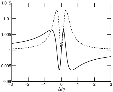
Figure 3: Refractive index (solid curve) and loss index (dashed curve) for an atomic cloud with a density $3.3\times 10^{12}({\rm cm}^{-3})$ corresponding the peak density of a trapped BEC at $T\approx 450$ (nK), slightly above $T_{C}$ [6]. Other parameters used are: $\lambda_{0}=589$ (nm), $\Gamma_{31}=0.5\gamma$, $\Gamma_{21}=(2\pi)10^{3}$ (Hz), $\Omega=0.56\gamma$, $\gamma=(2\pi)10.01$ (MHz).

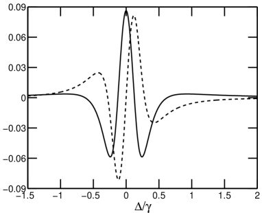
Figure 4: Group index (solid line) and phase correlation index (dashed line) (scaled by $1/c$) under the same conditions as Fig. 3.

In Fig. 4, we notice that $N_{g}^{\prime}$ has a local minimum at $\Delta\approx 0.3\gamma$. This local minima takes a negative value which signals a maximum negative delay time. However, in this case $N_{g}^{\prime\prime}$ is vanishingly small and it requires $L\rightarrow\infty$ to beat the absorption. With careful analysis, one can choose an optimum value of $N_{g}^{\prime}$ to take advantage of the amplification due to a nonzero $N_{g}^{\prime\prime}$. A typical simulation for the physical observable $U^{2}(z,t)$ is given in Fig. 5. For the parameters used, a temporal advancement of the pulse, in other words a negative delay of $7.5(\mu{\rm m})$ is found, which corresponds to a velocity higher than $c$ by $\sim 30({\rm m/s})$. It is possible to get higher superluminal velocities by decreasing the atomic vapor density. For instance, at $\rho=3.3\times 10^{10}({\rm cm}^{-3})$, which is $100$ times smaller than used in Figs. 3 and 5, the relevant parameters become $N_{g}^{\prime}=-3\times 10^{-4}c,N_{g}^{\prime\prime}=3\times 10^{-4}c$, and $\alpha^{\prime}=-1000({\rm 1/cm})$. In this case, superluminal tunneling occurs for $L>2({\rm cm})$. These parameters are experimentally accessible and in fact are close to reported values in a recent experiment [21], where $N_{g}^{\prime}=-8\times 10^{-5}c$ is measured in a Rb vapor of length $L=5({\rm cm})$.

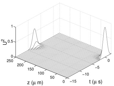
Figure 5: Superluminal pulse propagation, or tunneling through an EIT medium. The negative delay time of $7.5(\mu{\rm s})$ corresponds to a velocity higher than $c$ by $\sim 30$ (m/s).

To develop an operational theory for the slow light propagation as in the experiment [6], we need to include the above discussed amplitude-phase correlation as well as the non-uniform atomic gas density distribution. Furthermore, it would be necessary to include transverse diffraction losses as they might contribute significantly as the axial length of a trapped BEC increases. With all these complications, we have to resort to numerical simulations with available experimental parameters. Thus, we cannot simply define a group velocity for a pulse as $c/N_{g}^{\prime}$ or some other form. We should define a viable speed in accordance with the actual propagation of a physical pulse. In this article we follow the operational definition as used in experiments [6, 7]. We will concentrate on ultraslow pulse propagation rather than the equally likely superluminal effects.

The existence of amplitude-phase correlation calls for caution in interpreting both slow and fast light propagation in a dispersive or active medium. Straight forward conclusions based on a linear response theory and simple definitions of group velocities can not be taken very seriously, especially when conflicting view with non-locality properties of electromagnetic fields arise. Strictly speaking, a pulse is composed of Fourier superposition of infinite wave trains with potentially different phase velocities. It is meaningful only when there exists a finite bandwidth around central frequency so that we can write [22]

$$E(z,t)=\int_{k_{0}-\delta k}^{k_{0}+\delta k}E(k)e^{ikz-i\omega(k)t}dk.$$ (13)

Within a small bandwidth, linearization of the frequency around the center carrier gives $\omega(k)\approx\omega_{0}+v_{g}(k-k_{0})$ with $v_{g}=d\omega/dk$ (evaluated at $k_{0}$) the perceived group velocity. Such a velocity represents the speed of propagation of constant pulse amplitude surface, a non-existent situation when strong phase-amplitude correlation exists. The large cross phase-amplitude due to loss/gain index (or the imaginary part of the group velocity) causes ambiguity since the constant amplitude surface follows a trajectory now in the complex plane. As a result, we recommend treating the group velocity as a complex valued function. Further discussions will depend on specifics of medium’s electric susceptibility. This is the subject of the next section.

3 A Raman-matched EIT medium of cold atoms

Our study in this article is based on a medium of three-level $\Lambda$-type atoms. The excited level $|3\rangle$ is assumed to couple to the final state level $|2\rangle$ by a dressing laser beam with a Rabi frequency $\Omega$, and to the ground state $|1\rangle$ by the probe beam, whose propagation is the central issue of study. The dressing pump laser is assumed to be nearly Raman-matched with the probe laser (of carrier frequency $\omega_{0}$), which is detuned by $\Delta=\omega_{0}-\omega_{31}$ from the $|3\rangle\rightarrow|1\rangle$ transition frequency $\omega_{31}$. Initially all atoms are assumed to be in the ground state level $|1\rangle$. In the weak probe field limit, a linear response calculation can be carried as only a small fraction of atoms are pumped out of their initial state. In this study we use the approximation that the initial density profile $\rho_{1}(\vec{r})$ being unchanged. Solving the density matrix equation for atoms, we determine the linear susceptibility to be $\chi=\eta\chi_{1}$, directly related to the steady state value for the $|3\rangle\rightarrow|1\rangle$ matrix element. Here $\eta(\vec{r})=(3\lambda_{31}^{3}/32\pi^{3})\rho_{1}(\vec{r})$ and $\lambda_{31}$ is the transition wavelength and [3]

$$\chi_{1}(\Delta,\Omega)=-\left[\frac{\Delta}{\Gamma_{31}}+i\left(1+\frac{\Omega^{2}}{4\Gamma_{31}(\Gamma_{21}-i\Delta)}\right)\right]^{-1}.$$ (14)

$\Gamma_{31}$ is the decay rate from $|3\rangle$ to $|1\rangle$ and $\Gamma_{21}$ is the decoherence rate between $|2\rangle$ and $|1\rangle$. Typical detuning dependence of refractive and loss indices calculated from this susceptibility are shown in Fig. 3. The twin peaks in the loss index are from dressed absorption lines (Autler-Townes doublet [23]), and the narrow valley between them is associated with the normal dispersion region in the refractive index curve. Within the valley region, absorptive loss is vanishingly small. Far away from this lossless normal dispersion region both curves diminish resulting in a marked increase of transmission, except around the absorption peaks, where optical response is dominated by normal dispersion. Anomalous dispersion regions are accompanied by significant absorptive loss. For comparison, the group and phase correlation indices are illustrated in Fig. 4. In both normal and anomalous dispersion regions, we note that $N_{g}^{\prime}$ and $N_{g}^{\prime\prime}$ are now dominated by the term ($\partial\chi/\partial\Delta$) due to sharp variations in refractive and loss indices. In the normal dispersion region $N_{g}^{\prime}>0$, and particularly in the almost lossless region it attains a maximum on resonance,. This produces a minimal and well defined group velocity as $N_{g}^{\prime\prime}\approx 0$ in the same location. In the anomalous region $N_{g}^{\prime}$ becomes negative or zero, corresponding to vanishingly small or negative delay times of propagation, as recently observed in [9]. The frequency derivative $\partial\chi/\partial\Delta$ is found to be $\eta\partial\chi_{1}/\partial\Delta$ with

$$\frac{\partial\chi_{1}}{\partial\Delta}=\frac{\frac{1}{\Gamma_{31}}-\frac{\Omega^{2}}{4\Gamma_{31}(\Gamma_{21}-i\Delta)^{2}}}{\left[\frac{\Delta}{\Gamma_{31}}+i\left(1+\frac{\Omega^{2}}{4\Gamma_{31}(\Gamma_{21}-i\Delta)}\right)\right]^{2}}.$$ (15)

We can then define an auxiliary function $h(\Delta,\Omega)=\chi_{1}+(\Delta+\omega_{31})\partial\chi_{1}/\partial\Delta$, to express $N_{g}=1+2\pi\eta h(\Delta,\Omega)$. We note that $N_{g}^{\prime}$ is maximum on resonance, and the trapped atomic density profile peaks at $\vec{r}=0$. Therefore an estimate of the minimum for group speed is $v_{g}^{0}=c/[1+2\pi\eta(0)h^{\prime}(0,\Omega)]$. For a sample size of length $L$, we introduce dimensionless variables $\bar{z}=2z/L$ and $\bar{t}=(v_{g}^{0}/L)t$, and a normalized density profile function $f(\vec{r})=\rho_{1}(\vec{r})/\rho_{1}(0)$. In terms of these parameters, the wave equation Eq. (2) becomes

$$\frac{\partial{\cal E}}{\partial\bar{z}}+\left[\frac{v_{g}^{0}}{2c}+\frac{h(\Delta,\Omega)}{2h^{\prime}(0,\Omega)}f(\vec{r})\right]\frac{\partial{\cal E}}{\partial\bar{t}}=\frac{i\pi L}{2\lambda_{31}}\eta(0)\chi_{1}(\Delta,\Omega)f(\vec{r}){\cal E}.$$ (16)

In a typical experiment with $\Delta=0$ and $\Gamma_{31}\gg\Gamma_{21}$, we find

$$\chi_{1}(0,\Omega) \approx i\frac{4\Gamma_{31}\Gamma_{21}}{\Omega^{2}},$$

$$\left(\frac{\partial\chi_{1}}{\partial\Delta}\right)_{\Delta=0} \approx\frac{4\Gamma_{31}}{\Omega^{2}}.$$ (17)

Thus, $N_{g}^{\prime\prime}$ is indeed negligible and we have $N_{g}\approx 2\pi\omega_{31}\eta(4\Gamma_{31}/\Omega^{2})$. In this case, a well defined group velocity exists and is given by

$$v_{g}=c/N_{g}^{\prime}\approx\frac{4\pi^{2}\Omega^{2}c}{\rho 3\lambda_{31}^{3}\Gamma_{31}}\omega_{a}=\frac{\hbar c\epsilon_{0}\Omega^{2}}{2\omega_{31}d_{31}^{2}\rho}.$$ (18)

For convenience, the last expression is in SI units ($d_{31}^{2}/\hbar=3\lambda_{31}^{3}\Gamma_{31}/32\pi^{3}$). This result agrees with the one used for estimations of experimental results [6, 25]. It is also the same as obtained earlier [11, 26, 27, 28]. When applied to trapped atomic BEC at ultra low temperatures, inhomogeneous density profile needs to be included properly. When local density approximation is assumed, we expect the local light velocity should display rapid slowing down upon entering the BEC region from the thermal component and rapid acceleration when exiting it. This in general will result in different averaged velocity from simple estimations based on a uniform density. In order to elucidate this effect, it is necessary to specify an explicit form for the density profile of the BEC.

4 Spatial density profile of an interacting BEC

In this section, we review briefly a simple analytical model for the density profile of an interacting BEC as developed in Ref. [29]. We take the bose gas (below $T_{c}$) as composed of two components; a condensate part, whose density is computed using the Thomas-Fermi approximation and a background thermal atom part whose density is computed semi-classically assuming a continuum density of states in a harmonic trap [29, 30]. The total ground state density is then found to be

$$\rho_{1}(\vec{r})=\frac{\mu-V}{U}\theta(\mu-V)\theta(T_{C}-T)+\frac{g_{3/2}({\sf z}e^{-\beta V})}{\Lambda_{T}^{3}},$$ (19)

where $U=4\pi\hbar^{2}a_{\rm sc}/M$. $a_{\rm sc}$ is the atomic scattering length and $\theta(.)$ is the Heaviside step function, $g_{n}(x)=\sum_{j}x^{j}/j^{n}$, $\Lambda_{T}$ is the thermal de Bröglie wavelength and $\beta=1/(k_{B}T)$. The external trapping potential is $V(\vec{r})=M\omega_{r}^{2}(r^{2}+\epsilon^{2}z^{2})/2$ with $\omega_{r}$ the radial trap frequency and $\epsilon$ the aspect ratio. $M$ is atomic mass. The chemical potential $\mu$ is determined by the normalization $N=\int d\vec{r}\rho_{F}(\vec{r})$ with $N$ the total number of atoms. At high temperatures it is determined by solving ${\rm Li}_{3}({\sf z})=(T/T_{C})^{-3}\zeta(3)$ for fugacity ${\sf z}=e^{\beta\mu}$. ${\rm Li}_{3}(.)$ and $\zeta(3)$ are the third order polylogarithm and Riemann-Zeta functions respectively. At low temperatures, it is found that [29],

$$\mu=\mu_{TF}\left(\frac{N_{0}}{N}\right)^{2/5},$$ (20)

with $\mu_{TF}$ the Thomas-Fermi approximation to chemical potential and the condensate fraction

$$\frac{N_{0}}{N}=1-\left(\frac{T}{T_{C}}\right)^{3}-s\frac{\zeta(2)}{\zeta(3)}\left(\frac{T}{T_{C}}\right)^{2}\left[1-\left(\frac{T}{T_{C}}\right)^{3}\right]^{2/5},$$ (21)

with a scaling parameter $s$,

$$s=\frac{\mu_{TF}}{k_{B}T_{C}}=\frac{1}{2}\zeta(3)^{1/3}\left(15N^{1/6}\frac{a_{\rm sc}}{a_{ho}}\right)^{2/5}.$$ (22)

$a_{\rm ho}=\sqrt{\hbar/(M\epsilon^{1/3}\omega_{r})}$ denotes the average harmonic oscillator length scale [31].

5 Numerical results and discussion

In this section, we discuss several aspects of our numerical investigation for the experiment [6].

5.1 Group velocity in ideal and interacting BEC

According to experimental prescriptions [6, 7] we take the operational approach, first determine the delay time according to

$$t_{d}(T)=\frac{1}{\pi R^{2}}\int_{0}^{R}2\pi dr\int_{-L}^{L}dz\frac{1}{v_{g}(\vec{r})}-\frac{2L}{c},$$ (23)

where $R$ is the pinhole radius introduced to selectively detect propagated light from the near axial region of the atomic cloud. As justified before [24] we will ignore the spatial $(R)$ dependence of $L$ due to the shape of the cloud for small pinhole sizes and relatively long optical path length $L$ [25]. Within the local density approximation, the local group velocity is given by $v_{g}(\vec{r})=c/N_{g}^{\prime}$, and its average is then calculated according to $\langle v_{g}\rangle=L(T)/t_{d}(T)$ with $L(T)$ is the on-axis cloud size at a given temperature $T$. In Fig. 6 we compare the calculated results for an interacting and an ideal atomic gas.

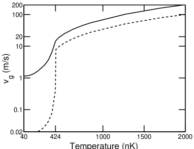
Figure 6: Comparison of an interacting (solid line) and ideal (dashed line) models for the temperature dependence of operationally defined group velocity. We have used the same parameters as in in Fig. 3. In addition, $N=8.3\times 10^{6}$, $a_{s}=2.75$ (nm), $\omega_{r}=(2\pi)69$ (Hz), $\omega_{z}=(2\pi)21$(Hz), $M=23$ (amu) as for the experiment [6]. $R_{0}=15$ ($\mu$m).

For the ideal gas case, our results simply reproduced those in Ref. [25]. Whenever possible we have used parameter values taken from Hau’s experiment [6]. At high temperatures both models are in agreement with the experimental data. At low temperatures, our model including atom-atom interaction gives results of the correct order of magnitude, while those based on ideal non-interacting atoms [25] are two orders of magnitude too low. We also note that the sharp low temperature dependence near the BEC transition temperature $T_{C}$ becomes significantly smoother, i.e. closer to the experimental observations when the atom interaction is included. Subsequently the calculated $\langle v_{g}\rangle$ does not fall down as rapidly at lower temperatures. Our model including atom-atom interaction also predicts that $\langle v_{g}\rangle$ increases with the atomic scattering length $a_{\rm sc}$ as illustrate in Fig. 7, where the group velocity is calculated for various scattering length parameters $a_{\rm sc}=7,5.75,3.75,1\,$(nm), corresponding to $s=0.3982,0.368,0.31,0.183$, respectively. We note that the two component density profile works particularly well for $s\ll 1$, but becomes less accurate when $s>0.3$ [29]. Thus, we conclude that the inclusion of interatomic interactions improves upon the ideal gas model prediction both qualitatively and quantitatively. In fact, our results with atom interaction give the correct order of magnitude as reported in the experiment [6]. Although we are still not near the reported value $v\sim 17\,({\rm m/s})$ for $T\sim 50\,({\rm nK})$. Inclusion of condensate number fluctuations, evaporation dynamics, and a self-consistent treatment of density profile might bring in further improvements.

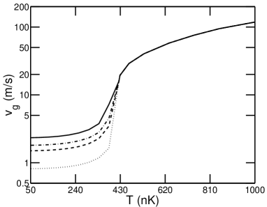
Figure 7: Group velocity is calculated with interacting BEC for $a_{\rm sc}=7,5.75,3.75,1$(nm) corresponding to solid, dot-dashed, dashed, and dotted curves, respectively. Other parameters are the same with those in Fig. 6.

5.2 Axial propagation of probe pulse

At temperatures well below $T_{C}$, both axial and radial density profiles of an atomic cloud are dominated by its condensate component. For the harmonic trapping potentials considered here, the Thomas-Fermi approximation results in an inverted paraboloid density profile. Consequently, the spatial behavior of the susceptibility in the linear response regime also follow such a behavior as shown in Fig. 8.

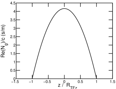
Figure 8: Axial profile of the scaled group index $N_{g}^{\prime}/c$ at $T=43$ (nK) and $\Delta=0$. $N_{g}^{\prime\prime}/c$ is very small with a peak value $\sim 10^{-12}$(s/m). All parameters are the same as in Fig. 6.

A typical simulation for the time delay of a resonant pulse $\exp{(-100t^{2})}$ after its passage through such a medium is is shown in Fig. 9.

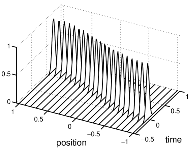
Figure 9: Propagation of a resonant pulse with $\Delta=0$, $T=43$ (nK). All parameters are the same as in Fig. 6. Position and time are given in dimensionless units explained in the text.

In this simple wave packet propagation, we only considered axial propagation along $z$. A discussion of paraxial effects and diffraction losses are given later in the next subsection. This one dimensional approach is shown to be valid in several recent slow pulse experiments where the incident Gaussian beam radius is much larger than the pinhole radius and the effects of the far radial tail become negligible. We find that upon entering the medium, the probe pulse rapidly slows down due to the sharply increased refractive index of the BEC component. It then propagates with a minimum speed around the center of the cloud, finally accelerates back to its initial vacuum speed as it exits near the edge of the cloud. According to this physical picture, the average delay which is used in determining the average group velocity is then lower than the optimal minimum group velocity at the trap center. Indeed, from the figure we see that the pulse arrives at the exit edge at about $0.6$ of the predicted delay time estimated from a uniform density. In Ref. [25], a group velocity of $9$ (m/s) was estimated for an interacting gas of effective uniform density with $N=10^{6}$ atoms, using the peak density from Thomas-Fermi approximation. When taking into account the condensate edge effects by directly propagating the wave equation in the scaled form, we obtained an improved estimation of $15$ (m/s), which agrees quite well with the reported value of $17$ (m/s). The average group velocity can be made very close to the desired minimum speed by choosing a density profile with sharp edges so that propagating light traverses the medium with the minimum speed for a longer fraction of total time spent in the medium. Ideally, a step function type density distribution along the axial direction would achieve this.

To complete this section, we also briefly studied absorption of the pulse. We examined the absorption length in detail using the propagation equation Eq.(16). At a large detuning of $\Delta=3\gamma$ we observe a penetration into only the first $15\%$ of the cloud as demonstrated in Fig. 10. By controlling the absorption length via detuning, interaction of light with only a selected part of the condensate might be realized in such a simple way.

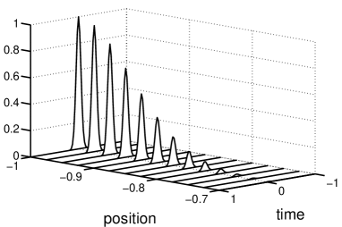
Figure 10: Absorption of an off-resonant pulse with detuning $\Delta=3\gamma$, $\gamma=(2\pi)10.01$ (MHz), and $T=43$ (nK). All other parameters are the same as in Fig. 6.Position and time are given in dimensionless units explained in the text.

5.3 Transverse diffraction effects

The discussion of radial density profile effects requires the inclusion of propagational diffraction. In practice, one can always choose appropriate trap parameters and suitably focused incident lasers to avoid most diffractive losses [6]. To examine the diffraction of a probe beam as it propagates through the condensate, we now include the previously neglected term $\nabla^{2}_{\bot}{\cal E}$ to the wave equation. Employing a standard pseudo-spectral split operator method for wave packet propagation [32] we have simulated the propagation of a pulse of radial cross section size $0.5$ (mm) in accordance with the experiment of Hau et al. [6]. Figure 11 illustrates its axial evolution of the time averaged intensity pattern.

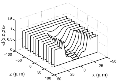
Figure 11: Diffraction pattern of a beam of radius 0.5 (mm) as it propagates through a Bose condensate at $T=0.3T_{C}$. All other parameters are the same as in Fig. 6.

In general, we find essentially one dimensional propagation equation Eq. (16) adequately describes near axis propagation as performed in the experiment [6, 7]. In the Fig. 11, we only plotted the $y=0$ plane because of its axial symmetry. Within the pinhole dimension set at $\sim 15\mu$m by experimental arrangement, and for detection close to the atomic cloud, diffraction effects are seen to be qualitatively negligible. Thus the large incident wave radius effectively assures a plane wave signal for the cloud size which is much smaller. The only significant effect of the transverse diffraction is then the diffraction loss of the pulse amplitude. In the experiment by Hau et al. [6], it was estimated that $80\%$ transmission of the probe pulse should occur under the EIT condition, yet even at high temperatures the observed transmission was limited to about $30\%$ [6]. Since Fig. 11 indicates a lower output intensity than found from the one dimensional axial propagation model, we suspect that the additional reduction in the pulse amplitude can be due to the transverse diffraction loss.

6 Conclusion

We have performed a detailed investigation of Raman-matched propagation of a probe laser pulse through a BEC. We have discussed of the interpretations and definitions of the group velocity, and argued that a complex valued group velocity should be used when strong amplitude-phase correlation exists. We have adopted the highly successful two component model for atomic condensate density profile and compared the differences of slow light propagation through an interacting and an ideal gas BEC. Based on the broadened condensate profile of an repulsively interacting Na atom BEC, we have obtained group velocity values of the same order of magnitude as observed in the experiment [6]. Furthermore our simulations for this experiment explains the qualitative behavior observed in the temperature dependence of the group velocity at low temperatures [6]. In the ultracold regime deep below the BEC transition temperature, including the atom-atom interaction and the inhomogeneous density profile results in two orders of magnitude improvement in the quantitative description of the group velocity behavior [25]. We also observed an increase in the group velocity at larger atomic scattering length.

When comparing the detailed spatial averaging of operationally defined delay time, we find that a sharp edged density profile yields lower average group velocity $\langle v_{g}\rangle$, i.e. closer to its local minimum $v_{g}(0)$, typically obtained based on the estimation of group velocity using the peak density. Our detailed numerical simulations confirm $\langle v_{g}\rangle\approx v_{g}(0)/0.6$, which gives essentially the same $\langle v_{g}\rangle$ value as reported [6].

We have also compared the One dimensional numerical simulations with a paraxial approximation including the diffraction effect during the probe pulse propagation. We find that under the experimental conditions, the use of a small pinhole to select probe light rays close to the x-axis is a reasonable approach as the diffractive effects are negligible apart from a total loss of the overall signal level. Thus, our studies also justify the one dimensional approach normally used in EIT studies.

7 acknowledgments

During the course of this work, one of us (L.Y.) was a participant of the recent workshop on quantum degenerate gases at the Lorentz Center, University of Leiden. L.Y. thanks H. Stoof for the hospitality. This work is supported by the NSF grant No. PHY-9722410.

References

- [1] C. Liu, Z. Dutton, C. H. Behroozi, and L. Vestergaard Hau, Nature 409, 490 (2001).
- [2] D. F. Phillips et al., Phys. Rev. Lett 86, 783 (2001).
- [3] S. E. Harris, Physics Today 50, 36 (1997); E. Arimondo, Progress in Optics (ed. E. Wolf), 257, (Elsevier Science, Amsterdam,1996).
- [4] M. O. Scully and M. S. Zubairy, Quantum Optics, (Cambridge University Press, 1997).
- [5] M. Fleischhauer and M. D. Lukin, Phys. Rev. Lett. 84, 5094 (2000).
- [6] L. V. Hau, S. E. Harris, Z. Dutton, and C. H. Behroozi, Nature 397, 594 (1999).
- [7] S. Inouye, R. F. Löw, S. Gupta, T. Pfau, A. Görlitz, T. L. Gustavson, D. E. Pritchard, and W. Ketterle, (cond-mat/0006455).
- [8] M. M. Kash, V. A. Sautenkov, A. S. Zibrov, L. Hollberg, G. R. Welch, M. D. Lukin, Y. Rostovtsev, E. S. Fry, and M. O. Scully, Phys. Rev. Lett. 82, 5229 (1999).
- [9] D. Budker, D. F. Kimball, S. M. Rochester, and V. V. Yashcuk, Phys. Rev. Lett. 83, 1767 (1999).
- [10] A. V. Turukhin, J. A. Musser, V. S. Sudarshanam, M. S. Shahriar, and P.R. Hemmer, (quant-ph/0010009).
- [11] S. E. Harris, J. E. Field, and A. Kasapi, Phys. Rev. A 46, R29 (1992).
- [12] M. D. Lukin and A. Imamoglu, Phys. Rev. Lett. 84, 1419 (2000).
- [13] M. D. Lukin, S. F. Yelin, and M. Fleischhauer, Phys. Rev. Lett. 84, 4232, (2000).
- [14] A. B. Matsko, Y. V. Rostovtsev, H. Z. Cummins, and M. O. Scully, Phys. Rev. Lett. 84, 5752 (2000).
- [15] M. Fleischhauer, M. D. Lukin, A. B. Matsko, and M. O. Scully, Phys. Rev. Lett. 84, 3558 (2000).
- [16] O. Kocharovskaya, Y. Rostovtsev, and M. O. Scully, (quant-ph/0001058).
- [17] F. Dalfovo, L. Pitaevskii, and S. Stringari, Phys. Rev. A 54, 4213 (1996).
- [18] S. E. Harris, J. E. Field, and A. Kasapi, Phys. Rev. A 46, R29 (1992).
- [19] R. Landauer and Th. Martin, Rev. Mod. Phys. 66, 217 (1994), and references therein.
- [20] A. M. Steinberg, P. G. Kwiat, and R. Y. Chiao, Phys. Rev. Lett. 71, 708 (1993); A. Enders and G. Nimtz, Phys. Rev. E 48, 632 (1993); R. Y. Chiao and A. M. Steinberg, Prog. Optics XXXVII, 345 (1997).
- [21] A. M. Akulshin, S. Barreiro, and A. Lezama, Phys. Rev. Lett. 83, 4277 (1999).
- [22] J. A. Stratton, Electromagnetic Theory, (McGraw-Hill, N.Y., 1941).
- [23] S. H. Autler and C. H. Townes, Phys. Rev. 100, 703 (1955).
- [24] Özgür Müstecaplıoḡlu and L. You, Phys. Rev. A (submitted, 2000).
- [25] G. Morigi and G. Agarwal, Phys. Rev. A 62, 013801 (2000).
- [26] R. Grobe, F. T. Hioe, and J. H. Eberly, Phys. Rev. Lett. 73, 3183 (1994).
- [27] M. Xiao, Y.-Q. Li, S.-Z. Jin, and J. Gea-Banacloche, Phys. Rev. Lett 74 666 (1995).
- [28] A. Kasapi, M. Jain, G. Y. Yin, and S. E. Harris, Phys. Rev. Lett. 74 2447 (1995).
- [29] M. Naraschewski and D. M. Stamper-Kurn, Phys. Rev. A 58, 2423 (1998).
- [30] V. Bagnato, D. E. Pritchard, and D. Kleppner, Phys. Rev. A 35, 4354 (1987).
- [31] S. Giorgini, L. P. Pitaevskii, and S. Stringari, Jour. Low Temperature Phys., 109, 309 (1997).
- [32] B. M. Garraway and K-A. Suominen, Rep. Prog. Phys. 58, 365 (19995).