Stimulated emission with a non-equilibrium state of radiation

Abstract

The stimulated emission from an atom interacting with radiation in non-equilibrium state is considered. The stochastic limit, applied to the non-relativistic Hamiltonian describing the interaction, shows that the state of atoms, driven by some non-equilibrium state of the field approaches a stationary state which can continuously emit photon, unlike the case with an equilibrium state.

Einstein applied Planck’s radiation theory to describe the equilibrium state between a atom and field[1]. He perceived that such an equilibrium state can be realized through the detailed balance condition, i.e. the balance in each mode between spontaneous and “stimulated emission”, i.e. the emission from the atom stimulated by the field. Einstein’s investigation can be said to give the clearest insight into the origin of Planck’s radiation because, with this notion, we can understand the Planck’s law on the density of states of the photons from an equilibrium field, i.e.

$$\rho(\omega)d\omega=\frac{\hbar\omega^{3}}{\pi^{2}c^{3}}\frac{1}{\exp\left(\frac{\hbar\omega}{kT}\right)-1}d\omega.$$ (1)

On the other hand, with the development of technology, a controlled emission with a controlled stimulating field has been realized in experimental situation, for example, a laser system. A laser is often described in terms of stimulated emission from an equilibrium state at negative temperature [2]. However the concept of the negative temperature can’t be accepted literally, but rather as an expediency to understand an inverse population state of the atoms which can emit photons. More precisely, a laser should be considered as a stimulated emission due to a non-equilibrium state of a field. In this letter we propose a way to understand such kind of stimulated emissions from non-equilibrium states, without introducing any phenomenological expediency like a negative temperature.

We apply the stochastic limit [3] to the non-relativistic QED Hamiltonian and derive two types of equations: one is the so-called rate equation for the atom and the other is an equation describing the time evolution of the number of photons. In addition, based on these equations, we discuss the stimulated emission from the atom interacting with some non-equilibrium field. The state of an atom driven by the non-equilibrium state of the field approaches a stationary state which can continuously emit photon, unlike the case of the equilibrium field. The conditions of the non-equilibrium state of the field for such phenomena is also made clear.

We shall consider an atom interacting with the EM-filed described with the standard non-relativistic QED Hamiltonian

$$H=H_{0}+\lambda~{}V,\quad H_{0}=H_{A}+H_{F}$$ (2)

where

$$H_{A}=\frac{p^{2}}{2m}+V(q),\quad\left([q,p]=i\right)$$ (3)

$$H_{F}=\int\omega(k)a^{\dagger}_{k,\sigma}a_{k,\sigma},~{}\quad\left([a_{k,\sigma},a^{\dagger}_{k^{\prime},\sigma^{\prime}}]=\delta_{\sigma\sigma^{\prime}}\delta(k-k^{\prime})\right)$$ (4)

and

$$V=\sum_{\sigma}\int dk\frac{1}{|k|^{1/2}}\varepsilon_{k,\sigma}\left(a_{\sigma,k}e^{ik\cdot q}+a_{\sigma,k}^{\dagger}e^{-ik\cdot q}\right).$$ (5)

$\sigma$ is polarization index ($\sigma=\leftrightarrow,\updownarrow$). In the following discussion we assume that $H_{A}$ has discrete spectrum or $H_{A}|\epsilon_{a}\rangle=\epsilon_{a}|\epsilon_{a}\rangle$. The interaction Hamiltonian in interaction picture $V(t)$ can be witten as [4]

$$V(t)=\sum_{\omega\in F}\sum_{a,b}\int dk\left(\overline{g_{ab}(k,\sigma)}E_{\omega}^{\dagger}\Big{(}|\epsilon_{a}\rangle\langle\epsilon_{b}|\Big{)}a_{k,\sigma}e^{-i(\omega(k)-\omega)t}+h.c\right)$$ (6)

where

$$\overline{g_{ab}(k,\sigma)} = \frac{1}{|k|^{1/2}}~{}\langle\epsilon_{a}|e^{ik\cdot q}p\cdot\varepsilon_{\sigma}|\epsilon_{b}\rangle,$$ (7)

$$E^{\dagger}_{\omega}(X) = \sum_{\epsilon_{r}\in F_{\omega}}P_{\epsilon_{r}}XP_{\epsilon_{r}-\omega},\quad P_{\epsilon_{r}}:=|\epsilon_{r}\rangle\langle\epsilon_{r}|$$ (8)

$$F = \{\omega=\epsilon_{r}-\epsilon_{r}^{\prime};~{}\epsilon_{r},\epsilon_{r}^{\prime}\in Spec~{}H_{A}\},\quad\mbox{(Bohr frequency)}$$ (9)

$$F_{\omega} = \{\epsilon_{r}\in Spec~{}H_{s};~{}\epsilon_{r}-\omega\in Spec~{}H_{A}\}.$$ (10)

We investigate the dynamics of the system described by the above Hamiltonian using the stochastic limit, which describes the quantum dynamics in the regime of weak coupling ($\lambda\rightarrow 0$) and large times ($t\rightarrow t/\lambda^{2}$) [3]. The main result of this theory (stochastic golden rule) [3] is that the time rescaling $t\rightarrow t/\lambda^{2}$ induces a rescaling of the quantum field

$$a_{k,\sigma}\rightarrow\frac{1}{\lambda}e^{-i\frac{t}{\lambda^{2}}(\omega(k)-\omega)}a_{k,\sigma}$$ (11)

and, in the limit $\lambda\rightarrow 0$ the rescaled field (11) becomes a quantum white noise (or master field) $b_{\omega,\sigma}(t,k)$ satisfying the commutation relations

$$[b_{\omega,\sigma}(t,k),b_{\omega^{\prime},\sigma^{\prime}}^{\dagger}(t^{\prime},k^{\prime})]=\delta_{\sigma\sigma^{\prime}}\delta_{\omega\omega^{\prime}}2\pi\delta(t-t^{\prime})\delta(\omega(k)-\omega)\delta(k-k^{\prime}).$$ (12)

Moreover, if the initial state of the field is the mean zero gauge invariant Gaussian state with correlations

$$\langle a^{\dagger}_{k}a_{k}^{\prime}\rangle=N(k)\delta(k-k^{\prime})$$

, then the state of the limit white noise will be of the some type with correlations

$$\langle b_{\omega,\sigma}(t,k)b_{\omega^{\prime},\sigma^{\prime}}^{\dagger}(t^{\prime},k^{\prime})\rangle = \delta_{\sigma\sigma^{\prime}}\delta_{\omega\omega^{\prime}}2\pi\delta(t-t^{\prime})\delta(\omega(k)-\omega)\delta(k-k^{\prime})N_{\sigma}(k)$$ (13)

$$\langle b^{\dagger}_{\omega,\sigma}(t,k)b_{\omega^{\prime},\sigma^{\prime}}(t^{\prime},k^{\prime})\rangle = \delta_{\sigma\sigma^{\prime}}\delta_{\omega\omega^{\prime}}2\pi\delta(t-t^{\prime})\delta(\omega(k)-\omega)\delta(k-k^{\prime})(N_{\sigma}(k)+1).$$ (14)

The Schrödinger equation becomes a quantum white noise equation which, after having been normally ordered, takes the form [3, 4]

$$dU_{t}=(-idH(t)-Gdt)U_{t}\quad;\quad t>0$$ (15)

with the initial condition $U_{0}=1$ and where $dH(t)$, called the martingale term, is the stochastic differential:

$$dH(t)=\sum_{\omega\in F}\sum_{a,b}\int dk\left(\overline{g_{ab}(k,\sigma)}E_{\omega}^{\dagger}\Big{(}|\epsilon_{a}\rangle\langle\epsilon_{b}|\Big{)}dB_{\omega,\sigma}(t)+E_{\omega}\Big{(}|\epsilon_{a}\rangle\langle\epsilon_{b}|\Big{)}dB_{\omega,\sigma}^{\dagger}(t)\right)$$ (16)

driven by the quantum Brownian motions

$$dB_{\omega,\sigma}=\sum_{\epsilon_{a}-\epsilon_{b}=\omega}\int^{t+dt}_{t}d\tau~{}\int dk\overline{g_{ab}(k,\sigma)}b_{\omega,\sigma}(\tau,k),$$ (17)

and the operator $G$, called the drift term, is given by

$$G=\sum_{\sigma}\sum_{\omega\in F}\left((g|g)^{-}_{\omega,\sigma}E^{\dagger}_{\omega}\Big{(}|\epsilon_{a}\rangle\langle\epsilon_{b}|\Big{)}E_{\omega}\Big{(}|\epsilon_{a}\rangle\langle\epsilon_{b}|\Big{)}+\overline{(g|g)}^{+}_{\omega,\sigma}E_{\omega}\Big{(}|\epsilon_{a}\rangle\langle\epsilon_{b}|\Big{)}E^{\dagger}_{\omega}\Big{(}|\epsilon_{a}\rangle\langle\epsilon_{b}|\Big{)}\right)$$ (18)

$$(g|g)^{-}_{\omega,\sigma} = \sum_{\epsilon_{a}-\epsilon_{b}=\omega}\int dk|g_{ab}(k,\sigma)|^{2}\frac{-i(N_{\sigma}(k)+1)}{\omega(k)-\omega-i0},$$ (19)

$$(g|g)^{+}_{\omega,\sigma} = \sum_{\epsilon_{a}-\epsilon_{b}=\omega}\int dk|g_{ab}(k,\sigma)|^{2}\frac{-iN_{\sigma}(k)}{\omega(k)-\omega-i0}.$$ (20)

With this quantum stochastic differential equation, we can always derive equations for the atom and field, that is, (i)master equation for reduced density operator for the atom, and (ii)equation for the field[4, 5].

One should notice that we do not assume the state of the field to be equilibrium. Therefore $N_{\sigma}(k)$ in (13) and (14) is not necessary to be

$$N_{\sigma}(k)=\frac{1}{e^{\beta\omega(k)}-1},~{}\left(\beta=\frac{1}{kT}\right),$$

but can be, for some general nonlinear functions $\beta_{\sigma}(\omega)$,

$$N_{\sigma}(k)=\frac{1}{e^{\beta_{\sigma}\left(\omega(k)\right)}-1}.$$ (21)

In this letter, let us consider a 3-level atom ($\epsilon_{1}<\epsilon_{2}<\epsilon_{3}$) whose matrix elements satisfy the conditions (Fig. 1)

$$\langle\epsilon_{1}|e^{ikq}p\cdot\varepsilon_{\updownarrow}|\epsilon_{2}\rangle=0,\quad\langle\epsilon_{2}|e^{ikq}p\cdot\varepsilon_{\leftrightarrow}|\epsilon_{3}\rangle=\langle\epsilon_{1}|e^{ikq}p\cdot\varepsilon_{\leftrightarrow}|\epsilon_{3}\rangle=0,\quad others\neq 0.$$ (22)

There are rather standard conditions in laser theory [2]. Notice however that condition (22) requires the preparation of the atom in a situation in which the longitudinal ($\updownarrow$) and transverse ($\leftrightarrow$) polarization do not enter symmmetrically. We believe that atoms, satisfying the condition (22), can be experimentally prepared. In addition, for simplicity, we restrict ourselves to a generic system [4]: this means in our case that the 3 Bohr frequencies $\omega_{21}$, $\omega_{31}$, $\omega_{32}$ ($\omega_{jk}=\epsilon_{j}-\epsilon_{k}$) are all different among themselves.

With these assumptions, we can derive the so-called rate equation for the atom

$$\frac{d}{dt}P_{1}(t) = -\left\{2(\gamma_{21,\leftrightarrow}^{(+)}+\gamma_{31,\updownarrow}^{(+)})P_{1}(t)-2(\gamma^{(-)}_{21,\leftrightarrow}P_{2}(t)+\gamma_{31,\updownarrow}^{(-)}P_{3}(t))\right\}$$ (23)

$$\frac{d}{dt}P_{2}(t) = -\left\{2(\gamma_{21,\leftrightarrow}^{(-)}+\gamma_{32,\updownarrow}^{(+)})P_{2}(t)-2(\gamma^{(-)}_{32,\updownarrow}P_{3}(t)+\gamma_{21,\leftrightarrow}^{(+)}P_{1}(t))\right\}$$ (24)

$$\frac{d}{dt}P_{3}(t) = -\left\{2(\gamma_{32,\updownarrow}^{(-)}+\gamma_{31,\updownarrow}^{(-)})P_{3}(t)-2(\gamma^{(+)}_{31,\updownarrow}P_{1}(t)+\gamma_{32,\updownarrow}^{(+)}P_{2}(t))\right\}$$ (25)

and the corresponding equations for polarized photons

$$\frac{d}{dt}n_{\leftrightarrow}(t) = 2~{}\left(\gamma^{(-)}_{21,\leftrightarrow}P_{2}(t)-\gamma^{(+)}_{21,\leftrightarrow}P_{1}(t)\right)$$ (27)

$$\frac{d}{dt}n_{\updownarrow}(t) = 2~{}\left(\gamma^{(-)}_{31,\updownarrow}P_{3}(t)-\gamma^{(+)}_{31,\updownarrow}P_{1}(t)+\gamma^{(-)}_{32,\updownarrow}P_{3}(t)-\gamma^{(+)}_{32,\updownarrow}P_{2}(t)\right)$$ (28)

where

$$P_{j}(t)=Tr\Big{(}\rho_{tot}(0)U^{\dagger}_{t}|\epsilon_{j}\rangle\langle\epsilon_{j}|U_{t}\Big{)},\quad n_{\sigma}(t)=Tr\Big{(}\rho_{tot}(0)U^{\dagger}_{t}\int dka^{\dagger}_{k,\sigma}a_{k,\sigma}~{}U_{t}\Big{)},$$ (29)

$$\gamma_{ij,\sigma}^{(\pm)}={\rm Re}(g|g)^{\pm}_{\omega_{ij},\sigma},$$ (30)

and the $(g|g)^{\pm}_{\omega_{ij},\sigma}$ are given by (19) and (20). Equations (LABEL:rate_equation) have a stationary solution which satisfies

$$\frac{P_{2}(\infty)}{P_{1}(\infty)} = \frac{\gamma_{31,\updownarrow}^{(-)}\gamma_{21,\leftrightarrow}^{(+)}+\gamma_{32,\updownarrow}^{(-)}\gamma_{21,\leftrightarrow}^{(+)}+\gamma_{31,\updownarrow}^{(+)}\gamma_{32,\updownarrow}^{(-)}}{\gamma_{31,\updownarrow}^{(-)}\gamma_{21,\leftrightarrow}^{(-)}+\gamma_{31,\updownarrow}^{(-)}\gamma_{32,\updownarrow}^{(+)}+\gamma_{32,\updownarrow}^{(-)}\gamma_{21,\leftrightarrow}^{(-)}}$$ (31)

$$\frac{P_{3}(\infty)}{P_{1}(\infty)} = \frac{\gamma_{31,\updownarrow}^{(+)}\gamma_{21,\leftrightarrow}^{(-)}+\gamma_{32,\updownarrow}^{(+)}\gamma_{21,\leftrightarrow}^{(+)}+\gamma_{31,\updownarrow}^{(+)}\gamma_{32,\updownarrow}^{(+)}}{\gamma_{32,\updownarrow}^{(-)}\gamma_{21,\leftrightarrow}^{(-)}+\gamma_{31,\updownarrow}^{(-)}\gamma_{21,\leftrightarrow}^{(-)}+\gamma_{31,\updownarrow}^{(-)}\gamma_{32,\updownarrow}^{(+)}}$$ (32)

$$\frac{P_{3}(\infty)}{P_{2}(\infty)} = \frac{\gamma_{32,\updownarrow}^{(+)}\gamma_{21,\leftrightarrow}^{(+)}+\gamma_{31,\updownarrow}^{(+)}\gamma_{21,\leftrightarrow}^{(-)}+\gamma_{32,\updownarrow}^{(+)}\gamma_{31,\updownarrow}^{(+)}}{\gamma_{31,\updownarrow}^{(-)}\gamma_{21,\leftrightarrow}^{(+)}+\gamma_{32,\updownarrow}^{(-)}\gamma_{21,\leftrightarrow}^{(+)}+\gamma_{31,\updownarrow}^{(+)}\gamma_{32,\updownarrow}^{(-)}}.$$ (33)

The right-hand side of equation (27) shows that, if $\gamma^{(-)}_{21,\leftrightarrow}P_{2}(t)-\gamma^{(+)}_{21,\leftrightarrow}P_{1}(t)>0$, i.e. if

$$\frac{P_{2}(t)}{P_{1}(t)}>\frac{\gamma_{21,\leftrightarrow}^{(+)}}{\gamma_{21,\leftrightarrow}^{(-)}}$$ (35)

then, $n_{\leftrightarrow}(t)$ must increase. Also with the stationary state of the atom, $n_{\leftrightarrow}(t)$ must keep increasing if

$$\frac{P_{2}(\infty)}{P_{1}(\infty)}>\frac{\gamma_{21,\leftrightarrow}^{(+)}}{\gamma_{21,\leftrightarrow}^{(-)}}$$ (36)

is satisfied. This means that, if we can experimentally realize condition (36), then we can also realize a continuous emission of $\leftrightarrow$-photon from the atom, stimulated by a non-equilibrium state of the field. Using (31), the condition (36) can be written as

$$\frac{\gamma_{21,\leftrightarrow}^{(+)}}{\gamma_{21,\leftrightarrow}^{(-)}}<\frac{\gamma_{31,\updownarrow}^{(-)}\gamma_{21,\leftrightarrow}^{(+)}+\gamma_{32,\updownarrow}^{(-)}\gamma_{21,\leftrightarrow}^{(+)}+\gamma_{31,\updownarrow}^{(+)}\gamma_{32,\updownarrow}^{(-)}}{\gamma_{31,\updownarrow}^{(-)}\gamma_{21,\leftrightarrow}^{(-)}+\gamma_{31,\updownarrow}^{(-)}\gamma_{32,\updownarrow}^{(+)}+\gamma_{32,\updownarrow}^{(-)}\gamma_{21,\leftrightarrow}^{(-)}}~{}~{}\Leftrightarrow~{}~{}\frac{\gamma_{21,\leftrightarrow}^{(+)}}{\gamma_{21,\leftrightarrow}^{(-)}}<\frac{\gamma_{31,\updownarrow}^{(+)}}{\gamma_{31,\updownarrow}^{(-)}}\frac{\gamma_{32,\updownarrow}^{(-)}}{\gamma_{32,\updownarrow}^{(+)}}.$$ (37)

If we suppose that the photon densities in the state (21) satisfy

$$N_{\leftrightarrow}(\omega)=N_{\updownarrow}(\omega)=\frac{1}{e^{\beta(\omega)}-1},$$

the condition (37) becomes equivalent to

$$\beta(\omega_{31})<\beta(\omega_{32})+\beta(\omega_{21}).$$ (38)

This process does not break the energy-conservation law. In fact one can easily check that

$$\frac{d}{dt}\left(\sum_{j=1}^{3}\epsilon_{j}P_{j}(t)+\sum_{\sigma}\int dk~{}\omega(k)Tr\Big{(}\rho_{tot}(0)U^{\dagger}_{t}a^{\dagger}_{k,\sigma}a_{k,\sigma}~{}U_{t}\Big{)}\right)=0,$$ (39)

and one should notice that the energy of the $\updownarrow$-field would be converted to the energy of the $\leftrightarrow$-field through the stationary state of the atom (Fig. 2). This is a peculiar property of the stimulated emission from a non-equilibrium state of the field. In fact the usual Gibbs states are characterized by the fact that the function $\beta$ in (21) is linear, i.e. $\beta(\omega)=\beta\omega$, and in this case condition (38) is never satisfied. The non-equilibrium field can therefore drive the atom to a stationary state which can emit photon, and this means that this stationary state gives an example of dissipative structure in the Prigogine sense [6].

In order to understand better the physical meanings of our condition (22), let us consider an extreme case such as

$$N_{\leftrightarrow}(\omega)\ll N_{\updownarrow}(\omega).$$ (40)

In this situation, the relation (31), defining the stationary solution, becomes approximately

$$\frac{P_{2}}{P_{1}} \sim \frac{\gamma_{31,\updownarrow}^{(+)}\gamma_{32,\updownarrow}^{(-)}}{\gamma_{32,\updownarrow}^{(-)}\gamma_{31,\updownarrow}^{(+)}}=\frac{N_{\updownarrow}(\omega_{32})}{N_{\updownarrow}(\omega_{32})+1}\frac{N_{\updownarrow}(\omega_{31})+1}{N_{\updownarrow}(\omega_{31})}\left(\neq\frac{N_{\updownarrow}(\omega_{21})}{N_{\updownarrow}(\omega_{21})+1},~{}\mbox{in general but Gibbs}\right)$$ (41)

$$\frac{P_{3}}{P_{1}} \sim \frac{\gamma_{31,\updownarrow}^{(+)}}{\gamma_{31,\updownarrow}^{(-)}}\qquad=\frac{N_{\updownarrow}(\omega_{31})}{N_{\updownarrow}(\omega_{31})+1}$$ (42)

$$\frac{P_{3}}{P_{2}} \sim \frac{\gamma_{32,\updownarrow}^{(+)}}{\gamma_{32,\updownarrow}^{(-)}}\qquad=\frac{N_{\updownarrow}(\omega_{32})}{N_{\updownarrow}(\omega_{32})+1}.$$ (43)

Notice that (41) is the Double Einstein formula discussed in [5] and that this stationary state is not a detailed balance but a distorted balance state. It is obvious that we need at least a 3-level atom to get such a distorted balance state because, since detailed balance means balance at each transition frequency, it follows that, if there is only one such frequency as in a 2-level atom, then every stationary state is a detailed balance state. This distorted balance state should play the role of the negative temperature state introduced in the phenomenology of laser systems[2]. Under the assumption (22) $\updownarrow$-field can be interpreted as the pumping field which realizes the so-called inverse population state of atom and the $\leftrightarrow$-field as a stimulating field which stimulates the emission from 2 to 1.

Finally, let us discuss to the stability of the non-equilibrium state of the field. With the above analysis, the non-equilibrium state seems extremely fragile against the interaction with atoms, while the equilibrium state seems robust. This difference should play an essential role to understand the dynamical properties of the nonequilibrium state of the field itself. It is an interesting problem to consider whether the non-equilibrium state after some interaction can become stable or not, and this problem should be related to the discussion on the stability of the macroscopic state. In order to approach these problems, we would have to take account of some kind of self-interaction of the field, that is the re-stimulation by the emitted photon, which we neglected in our discussion. Taking into account these effects, the equations of this system would be non-linear equations between $P_{i}(t)$, $n_{\sigma}(t)$ and other quantities, unlike in this letter. Our treatment in this letter is not sufficient to deal with the stability problem of the field. But in another application of the stochastic limit to superfluidity[7], a procedure to deal with this kind of self interaction has been already discussed and a non-linear equation has been derived. We think that we will be able to approach the stability problems of the non-equilibrium field also with a similar procedure.

The authors are grateful to I.V.Volovich for discussion. Kentaro Imafuku and Sergei Kozyrev are grateful to Centro Vito Volterra and Luigi Accardi for kind hospitality. This work was partially supported by INTAS 9900545 grant. Kentaro Imafuku is supported by a overseas research fellowship of Japan Science and Technology Corporation. Sergei Kozyrev was partially supported by RFFI 990100866 grant.

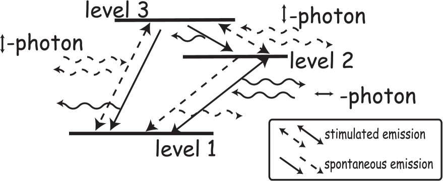
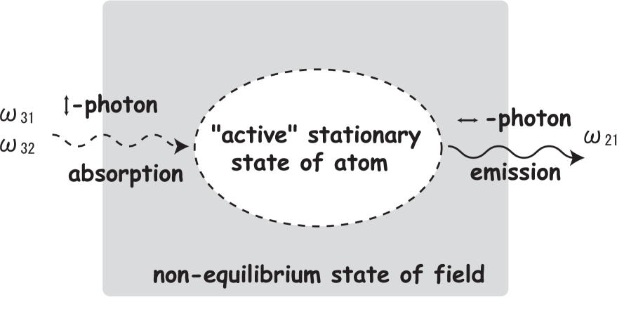
FIG. 1.: Schematical illustration of our assumption (22).

FIG. 2.: The energy flow from $\updownarrow$-photon to $\leftrightarrow$-photon.

REFERENCES

• [1] Einstein, A. Phys. Z. 18, 121 (1917)
• [2] See, e.g. H. Haken, In Encyclopedia of Physics, Vol. XXV/2c, Laser theory (Springer, Berlin-Heidelberg-New York 1970)
• [3] L.Accardi,  Y.G.Lu,  I.V.Volovich,  Quantum theory and its stochastic limit, Springer-Verlag (in press)
• [4] L.Accardi, S.V.Kozyrev,  Quantum interacting particle systems, Lecture Note of Levico school, September 2000, Preprint Centro Vito Volterra N.431
• [5] L.Accardi,  K.Imafuku,  S.V.Kozyrev, Interaction of 3-level atom with radiation, Preprint Centro Vito Volterra
• [6] P. Glansdorff, I.Prigogine, Thermodynamic theory of structure, stability and fluctuations (Wiley-Interscience, London, 1971)
• [7] L.Accardi,  S.V.Kozyrev, Superfluidity in the stochastic limit , Preprint Centro Vito Volterra.
Refer to caption