Biased EPR entanglement and its application to teleportation
Abstract
We consider pure continuous variable entanglement with non-equal correlations between orthogonal quadratures. We introduce a simple protocol which equates these correlations and in the process transforms the entanglement onto a state with the minimum allowed number of photons. As an example we show that our protocol transforms, through unitary local operations, a single squeezed beam split on a beam splitter into the same entanglement that is produced when two squeezed beams are mixed orthogonally. We demonstrate that this technique can in principle facilitate perfect teleportation utilising only one squeezed beam.
I Introduction
Entanglement is a key ingredient in many quantum communication tools [1]. It has been studied in dichotomic regimes such as photon-counting [2] and electron spin [3] and also in continuous variable regimes [4, 5]. Recently many of the quantum information protocols and tools developed dichotomically have been generalised to the continuous variable regime [6, 7, 8, 9, 10] and new experimental measures of continuous variable entanglement have also been proposed [11, 12, 13].
The most studied and generated form of entanglement in continuous variable quantum optics is Einstein-Podolsky-Rosen (EPR) entanglement [5, 14]. EPR entanglement is characterised by quantum correlations between conjugate quadrature amplitudes of two light beams. For example there may be quantum correlations between both the amplitude and the phase quadratures of the two beams. Usually EPR entanglement in which the correlations between conjugate quadratures are of equal strength is discussed. We will refer to this as unbiased EPR entanglement. There is no reason to restrict ourselves to this case however, and recently van Loock and Braunstein [15] examined entanglement with biased correlations. They evaluated the entanglement in terms of continuous variable teleportation of coherent states, studying two party and multi-party protocols.
In this paper we examine this type of entanglement in a more general way. Using a standard measure of EPR entanglement and introducing a new measure based on the number of photons present in a state, we show in what sense unbiased EPR entanglement is maximal. A key issue in our treatment is that of resources. That is, the number of photons used to produce a particular level of entanglement. Although an integral part of discrete variable discussions of quantum information, the question of resources is not always explicit in continuous variable treatments. Here we define maximal EPR states as those that use the minimum resources (photons) necessary to produce a particular degree of correlation.
We then discuss how it is possible to move between biased and unbiased states using only local operations. Using the example of continuous variable teleportation we show that an improvement in efficacy occurs with our protocol. In general unbiased entanglement provides optimum results, however we also show that there are some special situations where biased entanglement is optimal.
Protocols for manipulating entanglement are common in discrete variable quantum information. Perhaps most useful is distillation, or as it is sometimes called, concentration of entanglement [16, 17]. Distillation is a process involving only local operations and classical communication which takes some number of weakly entangled particles to a smaller number of more entangled particles. The total entanglement cannot be increased by such a process, only the entanglement per particle. Continuous variable distillation protocols [10, 18] take some number of weakly entangled modes and produce a smaller number of more entangled modes. In contrast the operations desribed in this paper involve single mode manipulations.
The paper is arranged in the following way: Section II reviews the techniques for characterising and producing EPR entanglement and introduces EPR symmetrisation and the concept of non-maximal EPR states for continuous variables. In Section III our protocol to redistribute the quantum correlations is introduced and in Section IV we consider its application to teleportation as an example. The protocol is generalised to tri-partite entanglement in Section V and we conclude in Section VI.
II Continuous variable entanglement
A Characterisation
An optical beam can be expressed as a mean unchanging field plus a fluctuation term [19].
| (1) |
Here is a field annihilation operator and is its expectation value. contains all of the fluctuations of the operator and can be split into two orthogonal hermitian operators, quadrature phase and quadrature amplitude . The superscripts and distinguish the phase and amplitude quadratures, respectively.
Taking the Fourier transform of produces the frequency domain operator which we denote by removing the hat. The variance of the phase and amplitude quadratures of an optical beam are given by . Throughout this paper we will consider sidebands at frequencies away from the carrier frequency and henceforth the frequency will not be shown explicitly. The Heisenberg uncertainty relationship can then be expressed in terms of these variances as .
In this paper the degree of quantum correlation between a given entangled pair of beams is measured with the product of conditional variances, , of conjugate quadratures between the two beams. This measure was first proposed by Reid and Drummond [5], is easily measureable, and has been used to characterise entanglement in a number of experiments [14, 20, 21]. The conditional variance measures how well a quadrature amplitude of one beam can be inferred from a quadrature measurement of the other beam, or in other words it measures the variance of the noise degrading the otherwise perfect correlations between the beams. By determining the conditional variances of two conjugate quadratures between beams, we may demonstrate the EPR-paradox experimentally [14]. This demonstration is a sufficient but not necessary condition for the states to be entangled (i.e inseparable). Limiting ourselves to the amplitude and phase quadratures, the condition for EPR entanglement becomes
| (2) |
where the conditional variances are given by [22] and the subscripts a and b label the two optical beams. defines a hard boundary below which the state must be entangled, the closer is to the stronger the entanglement. It is also possible to have rotated EPR correlations such that the conditional variance between (say) the amplitude of one beam and the phase of the other, and vice versa obey relations analogous to Eq.(2). We will only consider non-rotated states here.
A number of measures of entanglement are in useage. In particular the Duan criteria [13, 23] gives neccessary and sufficient conditions for separability of Gaussian states. We use the EPR condition here because of its physical significance and links with the efficacy of continuous variable quantum information protocols [24]. We mainly restrict ourselves in this paper to pure states and exclusively to Gaussian states. For pure Gaussian states the EPR condition is qualitatively equivalent to Duan’s criteria.
B Production
Continuous variable entanglement of the EPR type may be produced by mixing two squeezed beams on a 50/50 beam splitter [25, 26, 27]. Squeezed beams are ones for which or vice versa [19]. Throughout this paper we denote the input beams to this beam splitter by the subscripts 1 and 2, and the output beams by EPR1 and EPR2. For zero phase difference between the inputs at the beam splitter, the output quadrature amplitude relations are given by
| (3) | |||||
| (4) |
and the conditional variances between these two outputs are
| (5) |
If both input beams (1 and 2) are pure (minimum uncertainty) states, then
| (6) |
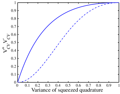
Now if both input beams are equally squeezed and the squeezing is in orthogonal directions (eg or ) then the output beams will be in the usual, unbiased, EPR entangled state. If the squeezing is not equal for the two beams and/or is not on orthogonal quadratures then biased entanglement will be produced. An interesting case is when only one input is squeezed (say and ). From equation (6) we find that is still less than 1 and thus the outputs are still entangled in this case. In this paper we will use this entanglement as our example, however the analysis and techniques we discuss can equally be applied to general biased entanglement. Clearly, for a fixed amount of squeezing, two squeezed beams will produce stronger correlations than one. Figure 1 shows for variable squeezing in both cases. As the squeezing strength increases, the biased and unbiased entanglement both approach perfect, .
As well as access to stronger correlations, entanglement from two squeezed beams has another advantage. Many quantum information protocols require quantum correlations in two conjugate quadratures, , which this entanglement naturally provides. Entanglement from only one squeezed beam on the other hand provides quantum correlations in only one quadrature, say but necessarily . One such example, is quantum teleportation of a coherent state where perfect entanglement from one squeezed beam () provides a fidelity of only compared with for perfect unbiased entanglement [15]. In section III we will show how perfect teleportation can be achieved utilising only one squeezed beam but first we would like to study the difference between biased and unbiased entanglement in more detail.
C EPR Symmetrisation
We now use a resource argument to define and quantify the difference between a maximal EPR state and a non-maximal EPR. We will identify unbiased entanglement as maximal.
First let us consider what we mean by “maximal” EPR. Clearly the maximum EPR state is the one for which . But creating such a state would require infinite energy, an unphysical limit. Thus the idea of a maximal EPR state should be considered within some limit on resources. Let us consider the minimum number of photons required to achieve a particular value of . We will define a maximal EPR state as one which achieves this particular value of entanglement with the minimum photon number. The average photon number in the sidebands of an optical beam, taken over some small range of frequencies for which the quadrature variances are constant, can be related to these variances (in suitably normalised units) via
| (7) | |||||
| (8) |
The quadrature variances of the individual EPR beams can be related to the conditional variances between them by invoking the uncertainty relations. If it is possible to infer the value of with a variance then the uncertainty relation requires that . Similarly if we can infer the value of with a variance then the uncertainty relation requires that . Thus
| (9) |
For pure-state entanglement expressions (9) are true in the equality, substituting these equalities into equation (7) we obtain the average photon number of each of the EPR beams
| (10) |
For a given degree of quantum correlation () the minimum value of is obtained when
| (11) |
and thus when the entanglement is unbiased. Both equation (11) and the equality of equation (9) are satisfied by entanglement produced from two minimum uncertainty equally squeezed beams. This identifies such states as maximal EPR states. Because for entanglement from a single squeezed beam we can immediately identify it as a non-maximal EPR state.
We describe the maximallity of the EPR entanglement by , the ratio of the minimum number of photons necessary (for that entanglement strength) to the number of photons present,
| (12) |
where is the mean photon number of the EPR state being analysed and is the mean photon number of the maximal EPR state with the same conditional variance product. If the state is maximal, if the state is non-maximal.
The parameter also identifies mixed states as non-maximal. Such states occur when the states used to produce the entanglement are not minimum uncertainty, or if the EPR beams suffer loss. For mixed states it is the equality of equation (9) which will not be satisfied, whilst the noise degrading the correlations may still be unbiased (i.e. ) . In the following discussion we will not consider mixed states further.
III Redistributing the quantum correlations
We introduce a method to transform pure non-maximal EPR states into maximal ones. In particular we will see how biased entanglement can be transformed into unbiased entanglement using only local unitary operations. These operations keep the overall degree of quantum correlation (as measured by ) constant whilst increasing (equation(12)).
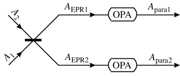
Let us consider the effect of passing entangled beams produced from only one squeezed beam through two independent degenerate optical parametric amplifiers (OPAs) as shown in figure 2. In the classical pump limit OPAs effect a unitary transformation of the field [19]. The effect of each OPA is to amplify the fluctuations of one of the input quadratures whilst de-amplifying the fluctuations of the orthogonal quadrature. The quadratures of amplification and de-amplification are controlled by the phase difference between the input and the pump field of the OPA. In our example, the amplitude quadratures of both beams are amplified. The effect of each OPA on its respective entangled beam is given by
| (13) | |||||
| (14) |
where the gain G has been chosen identically for both OPAs and the subscripts para1,2 label each entangled beam after the optical parametric operations. As the gain terms from each quadrature cancel on multiplication, these operations leave unchanged. After the OPAs the entangled quadratures given in equations (3) and (4) become
| (15) | |||||
| (16) | |||||
| (17) | |||||
| (18) |
We have previously stated that entanglement generated from one squeezed beam has quantum correlations in only one quadrature; two squeezed beams generate entanglement that has equal but weaker (for the same ) quantum correlations in both. For pure entanglement from one squeezed beam setting a gain (i.e. equal to the standard deviation of the anti-squeezed quadrature of the squeezed input beam) spreads the quantum correlations equally over both entangled quadratures. This makes the entanglement unbiased and in fact indistinguishable from entanglement generated from two squeezed beams. More generally a gain of
| (19) |
will make any pure EPR entanglement unbiased and thus maximal.
The OPAs are in fact acting as deamplifiers of photon number in this situation. By choosing the optimum gains we are able to reduce the photon number in the beams to the minimum allowed for their particular level of entanglement and thereby produce maximal entanglement. A physical picture of this process can be obtained by considering weak squeezed beams. Such beams can be described approximately in the Schrodinger picture as superpositions of vacuum and photon pairs: with . Mixing two of these beams on a beamsplitter with the appropriate phase relationship spatially separates the pairs into the individual beams producing the maximal entangled state . On the other hand splitting a single squeezed beam gives the state . We see that as well as the maximal component there is also a component of unseparated pairs. These do not contribute to the correlations. The effect of correctly tuned OPAs is to act as 2-photon absorbers which locally remove the 2-photon components leaving only the maximal component. A generalization of this argument to higher photon number orders can be made.
This process is similar to discrete variable concentration protocols [16] since the entanglement per photon is increased. Indeed there are strong similarities to the procrustean method of discrete concentration, where unentangled photons are “filtered out” whilst retaining the entangled ones [28]. However in the discrete case the photon is the fundamental carrier of the entanglement whilst in the continuous case it is the field mode which plays this role. In recognition of this distinction we refrain from using concentration to describe the continuous variable case.
IV Teleportation
In general the goal of quantum teleportation is to destroy a quantum state in one system and re-create it exactly in another. Many theoretical papers have been published on quantum teleportation [29] and it has been experimentally realised [27, 30, 31]. The Heisenberg uncertainty principle limits the information attainable from any two observables with a non-zero commutator relation [32]. Thus the perfect reproduction of an unknown input state via a direct measurment and recreation scheme is impossible. However a loophole exists if the sender, Alice, and receiver, Bob, share entanglement. This allows them to, in principle, teleport the state perfectly. The uncertainty principle is not violated as neither Alice nor Bob learn the identity of the teleported state.
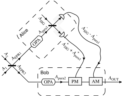
Figure 3 shows a typical continuous variable teleportation experiment with the addition of two local OPAs, one at Alices detection station and one at Bobs reconstruction station. The OPAs can conveniently be thought of as a local resource forming part of the teleportation protocol. The subscripts OUT and SIG label the the output and signal beams respectively. AM and PM label the amplitude and phase modulators respectively used to reconstruct the signal state with unity gain on one of the entangled beams. The input for the amplitude (phase) modulator is from an amplitude (phase) detector with suitably chosen gain.
The overlap integral of the original and teleported state Wigner functions is a measure of how similar the states are and is conventionally termed fidelity [33]. Other measures of teleportation quantify the disturbance (noise) introduced by the teleporter to an arbitrary teleported state under various conditions [26]. For ease of comparison with Ref.[15] we will use fidelity here and only consider unity gain (i.e. the teleportation gain has been chosen such that the size of the coherent displacement of the state before and after teleportation are equal).
If all noise sources are Gaussian, the fidelity of coherent state teleportation at unity gain is given by
| (20) |
The fidelity equals 1 when the Wigner function of the output state is a perfect replica of that of the signal state. The phase and amplitude variance of the output state of the teleporter shown in figure 3, assuming it functions perfectly, can be written as
| (21) | |||
| (22) |
We have assumed that the signal is coherent thus . This gives a fidelity of
| (23) |
The maximum fidelity for a given entanglement strength is obtained when the parametric gain is chosen as in equation (19) and is given by
| (24) |
This upper limit of achievable fidelity is set solely by the strength of the entanglement and, with appropriate parametric gain (dictated by equation (19)), all entanglement of equal strength (equal ) can in theory achieve it.
1 An example: Teleportation utilising biased entanglement
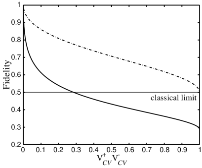
Consider entanglement generated from a single squeezed beam, for ideal squeezing approaches zero and thus the entanglement becomes perfect. Without specific OPA operations however, the maximum achievable fidelity (given by equation (23) with ,, and ) is [15]. After local OPA operations with G as in equation (19) the maximum fidelity (given by equation (24)) is equal to 1. Figure 4 shows the fidelity achieved first by simply using the biased entanglement and then by beforehand utilising our protocol to redistribute the quantum correlations.
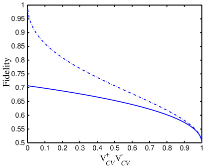
For reasonably strong squeezing substantial improvements in fidelity can be achieved via local OPA operations and indeed with just a single squeezed beam the teleportation can be perfect. In Ref.[15] the coherent state teleportation fidelity was taken as a measure of the entanglement. Remembering that entanglement cannot be increased by local operations, we see that coherent state fidelity only gives a lower bound to the entanglement strength.
2 Another example: Teleportation of a squeezed state
Here we consider teleportation of a squeezed state with an arbitrary coherent displacement. That is the orientation and dimensions of the squeezed ellipse are taken as constant and known, but the coherent displacement is unknown. We show that unbiased entanglement is not optimum in this case.
The fidelity of teleportation of a minimum uncertainty amplitude squeezed state with arbitrary coherent displacement is given by
| (25) |
where is the variance of the squeezed quadrature of the signal. Here the maximum fidelity is achieved when and is equal to that given in equation (24); again defines the classical limit. If unbiased entanglement is utilised in the teleporter and the gain simplifies to . So we see that to achieve the maximum fidelity it is now necessary to apply parametric gain to the entanglement, dependent on the strength of the signal squeezing. A comparison between the fidelity of teleportation of a squeezed state with , being teleported with entanglement generated from two equally squeezed beams, with and without OPA operations is shown in figure 5. Note that for unbiased entanglement as , which is less than 0.5 if . Thus quantum teleportation of a squeezed state with arbitrary coherent amplitude cannot be achieved with weak unbiased entanglement (see figure 5 for example).
This result can be thought of as redistribution of the quantum noise in such a way as to minimise the signal information gathered by the amplitude and phase quadrature measurements inside the teleporter. If the signal is strongly amplitude squeezed then the entanglement ‘noise’ must be increased in the anti-squeezed quadrature to hide its large quantum fluctuations and we can afford to decrease it in the squeezed quadrature because the squeezed fluctuations are small.
V Generalisation to Multi-partite Entanglement
We will now show that our protocol generalises to multi-party situations. In particular let us consider the continuous variable GHZ state [34, 15], so-called through analogy with the dichotomic GHZ state [35]. We can generalise the bipartite EPR condition to this tri-partite state by requiring that the amplitude and phase variances of, say, beam , conditioned on measurements of beams and , display an apparent violation of the Heisenberg uncertainty relation. The conditional variance generalised to the three beam situation is given by
| (28) | |||||
We can define a continuous variable GHZ violation as occurring when . This GHZ entanglement can be produced by combining three squeezed states on beam splitters such that the output fields (labelled GHZ1, GHZ2 and GHZ3) are given by
| (29) | |||||
| (30) | |||||
| (31) |
Gorbachev and Trubilko [34], and van Loock and Braunstein[15] consider GHZ states generated from three beams of equal squeezing with the squeezing of beam 1 orthogonal to that of beams 2 and 3, i.e. . This indeed satisfies the condition for GHZ violation for all levels of squeezing. However an examination of the correlations between the beams reveals they are biased in quadrature phase. A generalisation of the argument in Section IIC shows that pure GHZ states are maximal when this noise is unbiased. This can be arranged here by requiring that the squeezing of input beam one is stronger according to
| (32) |
This then produces a maximal GHZ state in the same sense as we defined a maximal EPR state. That is, for a given strength of GHZ entanglement this state has the least number of photons.
Now consider the situation of a single squeezed beam divided equally in three. This situation is described by equation (29) with beam 1 squeezed, say , but beam 2 and 3 in vacuum states . The GHZ condition is still satisfied for this state for any finite level of squeezing provided the squeezed input beam was in a minimum uncertainty state. This is in accordance with the conclusions of Ref. [15], though the state is clearly not maximal. However, as for the EPR case, it is possible to create a maximal GHZ state by applying OPAs, locally, to the three GHZ beams. In this case the required gain of the OPAs is
| (33) |
resulting in a maximal GHZ state indistinguishable from that produced from three squeezed states, as described by equation (32). These techniques can similarly be generalised to four or more parties.
VI Conclusion
We have studied pure state EPR entanglement in which the quantum correlations can be biased as a function of quadrature phase. We defined maximal EPR states as states having the most EPR entanglement for a given number of photons or equivalently as states with minimum photon number for a given value of . In particular we identified standard, unbiased EPR states produced from pairs of squeezed beams as maximal.
Entanglement produced from a single squeezed beam with squeezed variance was found to have the same degree of EPR correlation as entanglement from two squeezed beams with squeezed variances . Biased entanglement is non-maximal, however we identified local unitary operations which could convert it to a maximal EPR state of lower photon number but the same degree of correlation. We examined some consequences of these results as they apply to teleportation.
Finally we generalised our results to tri-partite entanglement. We identified the maximal continuous variable GHZ states. These are not produced from the superposition of three equally squeezed states. We showed that our techniques could be used to produce maximal GHZ states from the non-maximal one produced by equally dividing a single squeezed beam.
REFERENCES
- [1] C. H. Bennett and D. P. DiVincenzo, Nature 404, 247 (2000) and references therein.
- [2] For example see P. G. Kwiat, K. Mattle, H. Weinfurter, A. Zeilinger, A. V. Sergienko and Y. Shih, Phys. Rev. Lett. 75, 4337 (1995); J. Brendel, N. Gisin, W. Tittel and H. Zbinden, Phys. Rev. Lett. 82, 2594 (1999); J. D. Franson, Phys. Rev. A 45, 3126 (1992).
- [3] For example see A. Peres, Phys. Rev. A 54, 2685 (1996); N. Gisin, Phys. Lett. A 210, 151 (1996).
- [4] A. Einstein, B. Podolsky, N. Rosen, Phys. Rev. 47, 777 (1935).
- [5] M. D. Reid and P. D. Drummond, Phys. Rev. Lett. 60, 2731 (1988).
- [6] S. L. Braunstein and H. J. Kimble, Phys. Rev. Lett. 80, 869 (1998).
- [7] S. Lloyd and S. L. Braunstein, Phys. Rev. Lett. 82, 1784 (1999).
- [8] R. E. S. Polkinghorne and T. C. Ralph, Phys. Rev. Lett. 83, 2095 (1999).
- [9] T. C. Ralph, Phys. Rev. A 61, 010303(R) (1999).
- [10] L-M. Duan, G. Giedke, J. I. Cirac and P. Zoller, Phys. Rev. Lett. 84, 4002 (2000); L-M. Duan, G. Giedke, J. I. Cirac and P. Zoller, Phys. Rev. A 62, 032304 (2000).
- [11] K. Banaszek and K. Wódkiewicz, Phys. Rev. Lett. 82, 2009 (1999).
- [12] T. C. Ralph, W. J. Munro and R. E. S. Polkinghorne, Phys. Rev. Lett. 85, 2035 (2000).
- [13] L-M. Duan, G. Giedke, J. I. Cirac and P. Zoller, Phys. Rev. Lett. 84, 2722 (2000).
- [14] Z. Y. Ou, S. F. Pereira, H. J. Kimble, and K. C. Peng, Phys. Rev. Lett. 68, 3663 (1992).
- [15] P. van Loock, Samuel L. Braunstein, Phys. Rev. Lett. 84, 3482 (2000).
- [16] C. H. Bennett, H. J. Bernstein, S. Popescu and B. Schumacher, Phys. Rev. A 53, 2046 (1996).
- [17] C. H. Bennett, G. Brassard, S. Popescu, B. Schumacher, J. A. Smolin and W. K. Wootters, Phys. Rev. Lett. 76, 722 (1996).
- [18] S. Parker, S. Bose, M. B. Plenio, Phys. Rev. A 61, 032305 (2000).
- [19] D. F. Walls and G. J. Milburn, “Quantum Optics”, Springer-Verlag (1995).
- [20] Yun Zhang, Hai Wang, Xiaoying Li, Jietai Jing, Changde Xie, and Kunchi Peng, Phys. Rev. A 62, 023813 (2000).
- [21] Ch. Silberhorn, P. K. Lam, O. Weiss, F. Koenig, N. Korolkova, G. Leuchs, quant-ph/0103002.
- [22] M. J. Holland, M. J. Collett, D. F. Walls and M. D. Levenson, Phys. Rev. A 42, 2995 (1990).
- [23] G. Giedke, B. Kraus, M. Lewenstein, J. I. Cirac, Phys. Rev. Lett. 87, 167904 (2001).
- [24] Frederic Grosshans and Philippe Grangier, Phys. Rev. A 64, 010301 (2001).
- [25] G. Yeoman and S. M. Barnett, Journal Mod. Opt. 40, 1497 (1993).
- [26] T. C. Ralph and P. K. Lam, Phys. Rev. Lett. 81, 5668 (1998).
- [27] A. Furusawa, J. L. Sørensen, S. L. Braunstein, C. A. Fuchs, H. J. Kimble and E. S. Polzik, Science 282, 706 (1998).
- [28] R. T. Thew and W. J. Munro, Phys. Rev. A 63, 030302(R) (2001).
- [29] M. .B. Plenio and V. Vedral, Contemp. Phys 39, 6 (1998) and references within.
- [30] D. Bouwmeester, J. W. Pan, K. Mattle, M. Eibl, H. Weinfurter and A. Zeilinger, Nature 390, 575 (1997).
- [31] D. Boschi, S. Branca, F. De Martini, L. Hardy and S. Popescu, Phys. Rev. Lett. 80, 1121 (1998).
- [32] C. A. Fuchs and A. Peres, Phys. Rev. A 53, 2038 (1996).
- [33] B. Schumacher, Phys. Rev. A 51, 2738 (1995).
- [34] V. N. Gorbachev and A. I. Trubilko, quant-ph/9912061 (1999).
- [35] D. M. Greenberger, M. Horne, A. Shimony and A. Zeilinger, Am. J. Phys 58, 1131 (1990).