The local Larmor clock, Partial Densities of States, and Mesoscopic Physics

Abstract

Starting from the Larmor clock we introduce a hierarchy of density of states. At the bottom of this hierarchy are the partial densities of states which represent the contribution to the local density of states if both the incident and the out-going scattering channel is prescribed. We discuss the role of the partial densities of states in a number of electrical conduction problems in phase coherent mesoscopic systems: The partial densities of states play a prominent role in measurements with a scanning tunneling microscope on multiprobe conductors in the presence of current flow. The partial densities of states determine the degree of dephasing generated by a weakly coupled voltage probe. We show that the partial densities of states determine the frequency-dependent response of mesoscopic conductors in the presence of slowly oscillating voltages applied to the contacts of the sample. We introduce the off-diagonal elements of the partial density of states matrix to describe fluctuation processes. These examples demonstrate that the analysis of the Larmor clock has a wide range of applications.

1 Introduction

The Larmor clock is one of the most widely discussed approaches to determine the time-scales of tunneling processes. The essential ideaBAZ ; RYB ; LARMOR of the Larmor clock is that the motion of the spin polarization in a narrow region of magnetic field can be exploited to provide information on the time carriers spend in this region. It is assumed that incident carriers are spin polarized and that they impinge on a region to which a small magnetic field is applied perpendicular to the spin polarization of the incident carriers (see Fig. 1). The spin polarization of the transmitted and reflected carriers can then be compared with the polarization of the incident carriers. Dividing the angle between the polarization of the exciting carriers and that of the incident carrier by the Larmor frequency $\omega_{L}$ gives a time. Originally, only spin precession (the movement of the polarization in the plane perpendicular to the magnetic field) was considered. However, Ref. LARMOR pointed out, that especially if we deal with regions in which only evanescent waves exist (tunneling problems) the polarization executes not only a precession but also a rotation into the direction of the magnetic field. In fact in the presence of a tunneling barrier, the spin rotation, is the dominant effect. Ref. LARMOR considered a rectangular barrier and considered a magnetic field of the same spatial extend as the barrier. In the local version of the Larmor clock, introduced by Leavens and AersLEAE1 , we consider an arbitrary region in which the magnetic field is non-vanishing and investigate again the direction of the spin polarization and rotation of the transmitted and reflected carriers. The magnetic field might be non-vanishing in a small region localized inside the barrier or in a small region outside barrier on the side on which carriers are incident or on the far side of the barrier. We mention already here, that the response of the carriers is highly non-local: Even carriers which are reflected are affected by a magnetic field that is non-vanishing only on the far side of the barrier where naively we would expect only transmitted carriersLEAE2 .

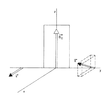
Figure 1: Spin polarized carriers incident on a barrier subject to a weak magnetic field $B_{0}$. The transmitted carriers exhibit both a spin precession and and a spin rotation. After LARMOR .

In this work we use the local Larmor clock to derive a set of local density of states states BU1 ; BTP ; BTP1 ; GASP ; GRAM which we call partial densities of states which are related to spin precession and in terms of sensitivities which are related to spin rotation. The partial densities of states, below abbreviated as PDOS, are useful to understand a number of transport problems: the transmission probability from a tunneling microscope tip into a multiterminal mesoscopic conductor GRAM can be expressed in terms of PDOS, the absorption of carriers by an optical potential (a potential with a small imaginary component), inelastic scattering and dephasing caused by a weak coupling voltage probe, and the low frequency transport in mesoscopic conductors.

The partial densities of states are determined by functional derivatives of the scattering matrix BU1 ; BTP ; GASP ; GRAM . Only in certain limited situations can the density of states be expressed in terms of energy derivatives. Expressions for the density of states in terms of energy derivatives of the scattering matrix are familiar dash ; avba . In the discussion of characteristic times the distinction between time-scales found from energy derivatives (like the Wigner-Smith phase delay) and time scales found from derivatives with respect to the local potential (the dwell time) has found some recognition. In contrast density of states are almost invariable discussed in terms of energy derivatives. Here we emphasize that a more precise discussion of density of states also uses derivatives with respect to the (local) potential and not energy derivatives. It is the dwell time (or sums of relevant dwell times) which are related to the density of states ianna1 ; ianna2 . The use of energy derivatives always signals that approximations are involved.

The interpretation of the Larmor clock remains a subject of discussion. Ref. LARMOR considered the total rotation angle dived by the Larmor precession frequency to be the relevant time. This interpretation brings the Larmor clock into agreement with the time-scales obtained by considering tunneling through a barrier with an oscillating potential Land . Subsequent works have argued that the precession angle and the rotation angle dived by the Larmor precession frequency separately should be viewed as time scales SOKOL ; GOR . The difficulty with such an interpretation is not only that one has two scales characterizing the same process, but the times defined in such a way are also not necessarily positive. Since we aim at characterizing a duration, that is a definite draw back. The two time scales can be combined into a complex time, with the real part referring to the precession time and the imaginary part to the time obtained from rotation. Like negative times, complex times are not part of the commonly accepted notions of time. Steinberg argues that the clock presents only a ”weak measurement” and that therefore complex times are permitted Stein . In quantum mechanics the questions ”how much time has the transmitted particle spent in a given interval” is problematic since being in an ”interval” and ”to be transmitted” corresponds to noncommuting operators muga . Reasonably, we can only speak of a time duration, if it is real and positive.

A comparison of the Larmor clock with the closely related linear ac-response of an electrical conductor shows immediately the ambiguity of the clock: in the ac-response of a conductor which is predominantly capacitive (tunneling limit) the voltage leads the current whereas for a highly transmissive conductor the response is inductive and the current leads the voltage.

The language used here implies similarly an extension of the usual notion of density of states. At the bottom of the hierarchy of density of states which we discuss are the partial densities of states (PDOS) which represents the contribution to the local density of states if we prescribe both the incident and the out-going channel. It turns out that certain partial densities of states are not positive. (These are of course just the PDOS that correspond to negative precession times). Thus the discussion presented below does not solve the interpretational questions related to the Larmor clock. Nevertheless as we will show even such negative PDOS are physically relevant. Using the partial densities of states, either by summing over the out-going channels (or by summing over the incident channels) we obtain the injectivity of a contact into a point within the sample or the emissivity of a point within the sample into a contact. Both injectivities and emissivities are positive and in the language of tunneling times correspond to local dwell times for which either the incident channel (or the outgoing channel but not both) are prescribed. Finally, if we take the sum of all the injectivities or the sum of all the emissivities we obtain the local density of states.

2 The scattering matrix and the local Larmor clock

We start by considering a one-dimensional scattering problem LARMOR ; LEAE1 ; LEAE2 . We consider particles moving along the $y$-axis in a potential $V(y)$. The potential is arbitrary, except that asymptotically, for large negative and large positive values of $y$ it is assumed to be flat. We adopt here the language from mesoscopic transport discussions and call the region of large negative $y$ the contact $1$ (the left contact) and the region of large positive $y$ contact $2$ (the right contact). We assume that the quantum mechanical evolution is described by the Schrödinger equation. A particle with energy $E$ has for large negative $y$ a wave vector $k_{1}(E)$ and a velocity $v_{1}(E)$ and for large positive values of $y$ a wave vector $k_{2}(E)$ and a velocity $v_{2}(E)$. We are interested in scattering states. A particle incident from the left is for large negative values of $y$ described by a scattering state

$$\psi_{1}(E,y)=e^{ik_{1}y}+S_{11}\,e^{-ik_{1}y}$$ (1)

and for large positive values of $y$ is described by a transmitted wave

$$\psi_{1}(E,y)=(\frac{v_{1}}{v_{2}})^{1/2}S_{21}\,e^{ik_{2}y}.$$ (2)

Similarly, a particle incident from the right is for large positive values of $y$ described by a scattering state

$$\psi_{2}(E,y)=e^{-ik_{2}y}+S_{22}\,e^{-ik_{2}y}$$ (3)

and for large negative values of $y$ is described by a transmitted wave

$$\psi_{2}(E,y)=(\frac{v_{2}}{v_{1}})^{1/2}S_{12}\,e^{ik_{2}y}.$$ (4)

Here the amplitudes $S_{\alpha\beta}$ determine the elements of the $2*2$-scattering matrix of the problem. Each scattering matrix element is a function of the energy $E$ of the incident carrier and is a functional of the potential $V(y)$. To express this dependence we write $S_{\alpha\beta}(E,V(y))$. Conservation of the probability current requires that this matrix is unitary and in the absence of a magnetic field time-reversal invariance implies that it is also symmetric.

Next we now consider a weak magnetic field applied to a small region. The magnetic field shall point into the $z$-direction. For simplicity we consider the case where the magnetic field is constant in a small interval $[y,y+dy]$ and takes there the value $B$. We consider only the effect of the Zeeman energy. Thus the motion of the particle remains one-dimensional and is as in the absence of a magnetic field confined to the $y$-axis. In the set-up for the Larmor clock, we consider particles with a spin. The spin of the incident particles (in the asymptotic regions) is polarized along the $x$-axis. For spin 1/2 particles the wave functions are now spinors with two components $\psi_{+}(y,E)$ and $\psi_{-}(y,E)$. Carriers incident from the left, have a spinor with components given by $\psi_{+}(y,E)=\psi_{-}(y,E)=({1/\sqrt{2}})exp(ik_{1}y)$. The Zeeman energy which is generated by the local magnetic field is diagonal in the spin up and spin down components. Consequently, in the interval $[y,y+dy]$ for a particle with spin up, the energy is reduced by $\hbar\omega_{L}/2$ with $\omega_{L}/2=g\mu B/\hbar$ and for a particle with spin down the potential is increased by $\hbar\omega_{L}/2$. Thus with the magnetic field switched on particles with spin up travel in a potential $V(y)-dV(y)$ and particles with spin down travel in potential $V(y)+dV(y)$. Here $V(y)$ is the potential in the absence of the magnetic field and $dV(y)$ is the potential generated by the magnetic field. Thus $dV(y)$ vanishes everywhere, except in the interval $[y,y+dy]$ where it takes the value $dV(y)=\hbar\omega_{L}/2=g\mu B$.

We can evaluate the polarization of the transmitted particles and the reflected particles if we can determine the scattering matrix for spin up and spin down particles in the potential generated by the magnetic field. Thus we need the scattering matrices $S^{\pm}_{\alpha\beta}(E,V(y)\mp dV(y))$ where $S^{+}$ is the scattering matrix for spin up carriers and $S^{-}$ is the scattering matrix for spin down carriers. Since the potential variation generated by the magnetic field is small we can expand these matrices away from the scattering matrix for the unperturbed potential. Thus we find to first order in the magnetic field for the scattering matrices

$$S^{\pm}_{\alpha\beta}(E,V(y))\mp dV(y))=S_{\alpha\beta}(E,V(y))\mp[dS_{\alpha\beta}(E,V(y))/dV(y)]dV(y)dy+.....$$ (5)

The variation of the scattering matrix due to the magnetic field is proportional to the derivative of the scattering matrix with respect to the local potential at the location where the magnetic field is non-vanishing. More generally, we can consider a magnetic field which varies along the $y$-axis (but always points along the $z$-axis). This leads to a potential $\delta V(y)$ determined by the local magnetic field. The variation of the scattering matrix is then determined by a functional derivative $[\delta s_{\alpha\beta}(E,V(y))/\delta V(y)]$ of the scattering matrix with regard to the local potential,

$$S^{\pm}_{\alpha\beta}(E,V(y))\mp\delta V(y))=S_{\alpha\beta}(E,V(y))$$ (6)

$$\mp\int dy^{\prime}[\delta s_{\alpha\beta}(E,V(y^{\prime}))/\delta V(y^{\prime})]\delta V(y^{\prime})+......$$ (7)

We emphasize that even though this equation looks quite simple, the evaluation of a functional derivative of a scattering matrix, while not difficult for a one-dimensional problem, can still be a laborious calculation.

Let us now find the precession and rotation angles of the polarization of the transmitted and reflected carriers. The normalized spinor of the transmitted particles which determines the spin orientation of the transmitted a particles has the components

$$\psi_{1+}(E,y)=\frac{S^{+}_{21}}{(|S^{+}_{21}|^{2}+|S^{-}_{21}|^{2})^{1/2}}.$$ (8)

$$\psi_{1-}(E,y)=\frac{S^{-}_{21}}{(|S^{+}_{21}|^{2}+|S^{-}_{21}|^{2})^{1/2}}.$$ (9)

First consider the polarization in the y direction. It is found by evaluating the expectation value of the Pauli spin matrix $\sigma_{y}$,

$$<s_{y}>_{21}=\frac{\hbar}{2}<\psi_{1}|\sigma_{y}|\psi_{1}>=-i\frac{\hbar}{2}\frac{S^{+\dagger}_{21}S^{-}_{21}-S^{+}_{21}S^{-\dagger}_{21}}{(|S^{+}_{21}|^{2}+|S^{-}_{21}|^{2})}.$$ (10)

Here the indices $21$ indicate that we consider transmission from left ($1$) to right ($2$) and evaluate the the spin in the transmitted beam. We need the spin polarization only to first order in the applied magnetic field. Using Eq. (6) we find

$$<s_{y}>_{21}=\frac{h}{T}\nu(2,y,1)\omega_{L}dy$$ (11)

where $T=|S_{21}|^{2}$ is the transmission probability in the absence of the magnetic field and

$$\nu(2,y,1)=-\frac{1}{4\pi i}\left(S_{21}^{\dagger}\frac{\delta S_{21}}{\partial V(y)}-\frac{\delta S_{21}^{\dagger}}{\delta V(y)}S_{21}\right)\;\;$$ (12)

is the partial density of states at $y$ of carriers which emanate from contact $1$ (the asymptotic region for large negative $y$) and eventually in the future reach contact $2$. Since initially the spin polarization was in the $x$-direction $<s_{y}>_{21}$ directly determines the angle of precession of the carriers in the $x-y$-plane. Thus by dividing $<s_{y}>_{21}$ by the Larmor precession frequency we can formally introduce a quantity with the dimension of time, which we call $\tau_{y}(2,y,1)$ and which is given by $\tau_{y}(2,y,1)=({h}/{T})\nu(2,y,1)dy.$ Here the index $y$ indicates that we deal with a time-scale obtained from the $y$-component of the spin polarization. We can now proceed to evaluate also the $y$-component of the spin polarization of the carriers which are reflected and can proceed to evaluate the $y$-component of the spin polarization of the carriers that are in the past incident from contact $2$ (large positive $y$) and in the future will be transmitted into contact $1$ (large negative $1$) or will be reflected back into contact $1$. We can summarize the results in the following manner: There are a total of four spin polarizations to be considered, each of them determined by a partial density of states

$$\nu(\alpha,y,\beta)=-\frac{1}{4\pi i}\left(S_{\alpha\beta}^{\dagger}\frac{\delta S_{\alpha\beta}}{\delta V(y)}-\frac{\delta S_{\alpha\beta}^{\dagger}}{\delta V(y)}S_{\alpha\beta}\right)\;\;$$ (13)

of carriers that are incident at contact $\beta=1,2$ and eventually in the future are transmitted or reflected into contact $\alpha=1,2$. Formally, the time scales related to precession in the local magnetic field at $y$ can be introduced which are related to the partial densities of states via, $\tau_{y}(\alpha,y,\beta)=({h}/{|S_{\alpha\beta}|^{2}})\nu(\alpha,y,\beta)dy$ where $|S_{\alpha\beta}|^{2}$ is the transmission probability $T$ if $\alpha$ and $\beta$ are not equal and is the reflection probability $R$ if $\alpha$ and $\beta$ are equal. Thus with each element of the scattering matrix we can associate a partial density of states. Later we discuss the properties of the partial densities of states in more detail.

Next we consider the spin polarization in the $z$-direction. For the carriers incident in contact $1$ and transmitted into contact $2$ we find that the $z$-component of the transmitted carriers is determined by

$$<s_{z}>_{21}=\frac{\hbar}{2}<\psi_{1}|\sigma_{z}|\psi_{1}>=\frac{\hbar}{2}\frac{|S^{+}_{21}|^{2}-|S^{-}_{21}|^{2}}{(|S^{+}_{21}|^{2}+|S^{-}_{21}|^{2})}.$$ (14)

Using Eq. (6) we find

$$<s_{z}>_{1}=\frac{h}{T}\eta(2,y,1)\omega_{L}dy.$$ (15)

where we call

$$\eta(2,y,1)=-\frac{1}{4\pi}\left(S_{21}^{\dagger}\frac{\delta S_{21}}{\delta U(y)}+\frac{\delta S_{21}^{\dagger}}{\delta U(y)}S_{21}\right)\;\;$$ (16)

the sensitivity of the scattering problem. Since the spin polarization of the incident particles was originally along the $x$-direction only a small $z$-component of the incident particle determines a spin rotation angle. We can formally introduce a time scale $\tau_{z}(2,y,1)$ associated with spin rotation which is given by $\tau_{z}(2,y,1)=({h}/{T})\eta(2,y,1)dy$. Again we can ask about the $z$-polarization of reflected particles and can ask about the $z$-polarization of particles incident from the right. The results are summarized by attributing each scattering matrix element $S_{\alpha\beta}$ a sensitivity

$$\eta(\alpha,y,\beta)=-\frac{1}{4\pi}\left(S_{\alpha\beta}^{\dagger}\frac{\delta S_{\alpha\beta}}{\delta U(y)}+\frac{\delta S_{\alpha\beta}^{\dagger}}{\delta U(y)}S_{\alpha\beta}\right)\;\;$$ (17)

which determine the time-scales $\tau_{z}(\alpha,y,\beta)=({h}/{|S_{\alpha\beta}|^{2}})\eta(\alpha,y,\beta)dy.$ Finally we can determine the spin polarization in the $x$-direction. This component is reduced from its initial value both because of spin precession in the $x-y$-plane and because of the rotation of spins into the $z$-direction. Since we have at every space point

$$<s_{x}>^{2}+<s_{y}>^{2}+<s_{z}>^{2}=\hbar^{2}/4,$$ (18)

it follows immediately that the time scale $\tau_{x}$ is related to the two time-scales introduced above by

$$\tau_{x}=(\tau_{y}^{2}+\tau_{z}^{2})^{1/2}.$$ (19)

Using the expressions for $\tau_{y}$ and $\tau_{z}$ given above, we find for the time-scales $\tau_{x}$ the following expressions

$$\tau_{x}(\alpha,y,\beta)=\frac{h}{|S_{\alpha\beta}|^{2}}\left(\frac{\delta S_{\alpha\beta}}{\delta V(y)}\frac{\delta S_{\alpha\beta}^{\dagger}}{\delta V(y)}\right)^{1/2}.\;\;$$ (20)

We reemphasize that neither the partial densities of states nor the sensitivities are in general positive. In contrast, $\tau_{x}(\alpha,y,\beta)$ is positive for all elements of the scattering matrix.

3 Absorption and Emission of Particles: Injectivities and Emissivities

Before discussing the partial densities of states in more detail it is of interest to investigate the absorption of particles in a small scattering region MB90 . We assume that in a narrow interval $[y,y+dy]$ there exists a non-vanishing absorption rate $\Gamma$. Thus the potential $V(y)$ is equal to $V_{0}(y)-i\hbar\Gamma$ in the interval $[y,y+dy]$ and is equal to $V_{0}(y)$ out-side this interval. To solve the scattering problem we need to find the scattering matrix $S^{\Gamma}_{\alpha\beta}(E,V(y))$ in the presence of this complex potential $V(y)$. Of interest here is, as in Ref. MB90 , the limit of small absorption. The case of strong absorption is also of interest but thus has been used only to discuss global properties and not the local quantities of interest here rama ; been . For a small absorption rate we can expand the scattering matrix $S^{\Gamma}_{\alpha\beta}(E,V(y))$ in powers of the absorption rate away from the scattering problem in the original real potential $V_{0}$. We obtain

$$S^{\Gamma}_{\alpha\beta}(E,V(y))=S_{\alpha\beta}(E,V_{0}(y))$$ (21)

$$+i\hbar[\delta S_{\alpha\beta}(E,V(y))/\delta V(y)]|_{V(y)=V_{0}(y)}\Gamma dy+.....$$ (22)

We note that the adjoint scattering matrix has to be evaluated in the potential $V^{*}(y)$ and hence

$$S^{\Gamma\dagger}_{\alpha\beta}(E,V(y))=S^{\dagger}_{\alpha\beta}(E,V_{0}(y))$$ (23)

$$-i\hbar[\delta S^{\dagger}_{\alpha\beta}(E,V(y))/\delta V(y)]|_{V(y)=V_{0}(y)}\Gamma dy+....$$ (24)

With these results it easy to show that the transmission and reflection probabilities in the presence of a small absorption in the interval $[y,y+dy]$ are

$$|S^{\Gamma}_{\alpha\beta}(E,V(y))|^{2}=|S_{\alpha\beta}(E,V_{0}(y))|^{2}(1-\Gamma\nu(\alpha,y,\beta)dy)$$ (25)

where $|S_{\alpha\beta}(E,V_{0}(y))|^{2}$ is the transmission probability $T$ of the scattering problem without absorption if $\alpha$ and $\beta$ are different and is the reflection probability $R$ of the scattering problem without absorption if $\alpha=\beta$. The incident current $j_{in}$, must be equal to the sum of the transmitted current $j_{T}$, the reflected current $j_{R}$ and the absorbed current $j_{\Gamma}$,

$$j_{in}=j_{T}+j_{R}+j_{\Gamma}.$$ (26)

Using Eq. (21) and taking into account that the incident flux is normalized to $1$, we find for carriers incident from the left or right $\beta=1,2$ an absorbed flux given by

$$j_{\Gamma}(y,\beta)=\Gamma\nu(y,\beta)dy,$$ (27)

where $\nu(y,\beta)$ is called the injectivity of contact $\beta$ into point $y$. The injectivity of the contact is related to the partial densities of states via

$$\nu(y,\beta)=\sum_{\alpha}\nu(\alpha,y,\beta).$$ (28)

In our problem with two contacts the injectivity is just the sum of two partial densities of states.

Another way of determining the absorbed flux proceeds as follows. The absorbed flux is proportional to the integrated density of particles in the region of absorption (in the interval $[y,y+dy]$). The density of particles can be found from the scattering state $\psi_{\beta}(y)$ given by Eqs. (1 -4). For carriers incident from contact $\beta$ the absorbed flux is thus

$$j_{\Gamma}(y,\beta)=\Gamma\frac{1}{hv_{\beta}}|\psi_{\beta}(y)|^{2}dy.$$ (29)

Note that here the density of states $1/hv_{\beta}$ of the asymptotic scattering region appears. It normalizes the incident current to $1$. Thus we have found a wave function representation for the injectivity. Comparing Eq. (26) and Eq. (25) gives

$$\nu(y,\beta)=\frac{1}{hv_{\beta}}|\psi_{\beta}(y)|^{2}.$$ (30)

The total local density of states $\nu(y)$ at point $y$ is obtained by considering carriers incident from both contacts. In terms of wave functions $\nu(y)$ is for our one-dimensional problem given by

$$\nu(y)=\sum_{\beta}\frac{1}{hv_{\beta}}|\psi_{\beta}(y)|^{2}.$$ (31)

Thus the total density of states is also the sum of the injectivities from the left and right contacts

$$\nu(y)=\sum_{\beta}\nu(y,\beta).$$ (32)

There is now an interesting additional problem to be addressed. Instead of a potential which acts as a carrier sink (as an absorber) we can ask about a potential which acts as a carrier source. Obviously, all we have to do to turn our potential into a carrier source is to change the sign of the imaginary part of the potential. With a a carrier source in the interval $[y,y+dy]$ we should observe a particle current toward contact $1$ and a particle current toward contact $2$. We suppose that carriers are incident both from the left and the right and evaluate the currents in the contact regions. The total current injected into the sample at $y$ is

$$j_{in}(y)=\Gamma\nu(y)dy.$$ (33)

Taking into account that the incident current is normalized to $1$ the current $j_{out}(\beta,y)$ in contact $\beta$ due to a carrier source at $y$ is given by

$$j_{out}(\alpha,y)=1-\sum_{\beta}|s^{\Gamma}_{\alpha\beta}(E,V(y))|^{2}$$ (34)

due to the modification of both the transmission and reflection coefficients. Using Eq. (21) (with $\Gamma$ replaced by -$\Gamma$) gives

$$j_{out}(\alpha,y)=-\Gamma\sum_{\beta}\nu(\alpha,y,\beta)\,dy=-\Gamma\nu(\alpha,y)\,dy.$$ (35)

The current in contact $\alpha$ is determined by the emissivity $\nu(\alpha,y)$ of the point $y$ into contact $\alpha$. Note the reversal of the sequence of arguments in the emissivity as compared to the injectivity. Thus the emissivity is like the injectivity a sum of two partial densities of states,

$$\nu(\alpha,y)=\sum_{\beta}\nu(\alpha,y,\beta).$$ (36)

For a scattering problem in the absence of a magnetic field the injectivity and emissivity are identical. If there is a homogeneous magnetic field present they are related by reciprocity: the injectivity from contact $\alpha$ into point $y$ is equal to the emissivity of point $y$ into the contact $\alpha$ in a magnetic field that has been reversed, $\nu_{+B}(y,\alpha)=\nu_{-B}(\alpha,y)$.

We have thus obtained a hierarchy of density of states: At the bottom are the partial densities of states $\nu(\alpha,y,\beta)$ for which we describe both the contact from which the carriers are incident and the contact through which the carriers have to exit. On the next higher level are the injectivities $\nu(y,\alpha)$ and the emissivities $\nu(\alpha,y)$. For the injectivity we prescribe the contact through which the carrier enters but the final contact is not prescribed. In the emissivity we prescribe the contact through which the carrier leaves but the incident contact is not prescribed. Finally, on the highest level is the local density of states $\nu(y)$ for which we prescribe neither the incident contact nor the contact through which carriers leaves.

For simple scattering problems (delta-functions, barriers) the interested reader can find a derivation and discussion of partial densities of states in Refs. GASP ; GRAM ; zhao .

Returning to time scales: we have shown that the partial densities of states are associated with spin precession. It is tempting, therefore, to associate them with a time duration. However, as can be shown, the partial densities of states are not necessarily positive. (The simple example of a resonant double barrier shows that one of the diagonal elements $\nu(\alpha,y,\alpha)$ has a range of energies where it is negative MB90 ). The injectivities and emissivities are, however, always positive. The proof is given by Eq. (28). We can associate a local dwell time $\tau_{D}(y,\beta)=\hbar\nu_{D}(y,\beta)$ with the injectivity which gives the time a carrier incident from contact $\beta$ spends in the interval $[y,y+dy]$ irrespective of whether it is finally reflected or transmitted. Similarly, we can associate a dwell time with the emissivity which is the time carriers spend in the interval $[y,y+dy]$ irrespective from which contact they entered the scattering region. There is little question that the dwell times have the properties which we associate with the duration of a process: they are real and positive. However, as explained they do not characterize transmission or reflection processes.

4 Potential Perturbations

Thus far our discussion has focused much on the partial densities of states. The sensitivity introduced as a measure of the spin rotation in the Larmor clock has, however, also an immediate direct interpretation. We have seen that the partial densities of states are obtained in response to a complex perturbation of the original potential $V(y)$. The sensitivity comes into play if we consider a real perturbation $\delta V$ of the original potential. Thus if we consider a potential which is equal to $V(y)+\delta V$ in the interval $[y,y+dy]$ and equal to $V(y)$ elsewhere the transmission probability $T^{V}$ in the presence of the perturbation is $T^{V}=T+4\pi\eta(\alpha,y,\beta)\delta Vdy$, with $\alpha\neq\beta$. The reflection probability is $R^{V}=R+4\pi\eta(\alpha,y,\alpha)\delta Vdy$. Since also $T^{V}+R^{V}=1$ we must have $\eta(y)\equiv\eta(\alpha,y,\beta)=-\eta(\alpha,y,\alpha)$. For our scattering problem, described by a $2*2$ scattering matrix there exists only one independent sensitivity $\eta(y)$. In the Larmor clock the sensitivity corresponds to spin rotation and the fact that there is only one sensitivity follows from the conservation of angular momentum: the weak magnetic field cannot produce a net angular momentum. If carriers in the transmitted beam acquire a polarization in the direction of the magnetic field then carriers in the reflected beam must have a corresponding polarization opposite to the direction of the magnetic field. In mesoscopic physics, in electrical transport problems, the sensitivity plays a role in the discussion of non-linear current-voltage characteristics and plays a role if we ask about the change of the conductance in response to the variation of a gate voltage br2 . Below, we will not further discuss the sensitivity, but we will present a number of examples in which the partial densities of states play a role.

5 Generalized Bardeen formulae

It is well known that with a scanning tunneling microscope (STM) we can measure the local density of states STM . STM measurements are typically performed in a two terminal geometry, in which the tip of the microscope represents one contact and the sample provides another contact STM . Here we consider a different geometry. We are interested in the transmission probability from an STM tip into the contact of a sample with two or more contacts as shown in Fig. 2. Thus we deal with a multiterminal transmission problem GRAM . If we denote the contacts of the sample by a Greek letter $\alpha=1,2,..$ and use tip to label the contact of the STM tip, we are interested in the tunneling probabilities $T_{\alpha tip}$ from the tip into contact $\alpha$ of the sample. In this case the STM tip acts as carrier source. Similarly we ask about the transmission probability $T_{tip\alpha}$ from a sample contact to the tip. In this case the STM tip acts as a carrier sink. Earlier work has addressed this problem either with the help of scattering matrices, electron wave dividers, or by applying the Fermi Golden Rule. Recently, Gramespacher and the author GRAM have returned to this problem and have derived expressions for these transmission probabilities from the scattering matrix of the full problem (sample plus tip). For a tunneling contact with a density of states $\nu_{tip}$ which couples locally at the point $x$ with a coupling energy $|t|$ these authors found

$$T_{tip,\alpha}=4\pi^{2}\,\nu_{tip}\,|t|^{2}\,\nu(x,\alpha)\,,$$ (37)

$$T_{\alpha tip}=4\pi^{2}\,\nu(\alpha,x)\,|t|^{2}\,\nu_{tip}\,.$$ (38)

In a multiterminal sample the transmission probability from a contact $\alpha$ to the STM tip is given by the injectivity of contact $\alpha$ into the point $x$ and the transmission probability from the tip to the contact $\alpha$ is given by the emissivity of the point $x$ into contact $\alpha$. Eqs. (37) and (38) when multiplied by the unit of conductance $e^{2}/h$ are generalized Bardeen conductances for tunneling into multiprobe conductors. Since the local density of states of the tip is an even function of magnetic field and since the injectivity and emissivity are related by reciprocity we also have the reciprocity relation $T_{tip,\alpha}(B)=T_{\alpha,tip}(-B)$.

The presence of the tip also affects transmission and reflection at the massive contacts of the sample. To first order in the coupling energy $|t|^{2}$ these probabilities are given by

$$|S^{tip}_{\alpha\beta}|^{2}=|S_{\alpha\beta}|^{2}-4\pi^{2}\,\nu(\alpha,x,\beta)\,|t|^{2}\,\nu_{tip}\,.$$ (39)

The correction to the transmission probabilities $\alpha\neq\beta$ and reflection probabilities $\alpha=\beta$ is determined by the partial densities of states, the coupling energy and the density of states in the tip. Note that if these probabilities are placed in a matrix then each row and each column of this matrix adds up to the number of quantum channels in the contacts.

Figure 2: Partial density of states measurement with a scanning tunneling microscope. The tip of an STM couples at a point $x$ with a coupling strength $t$ to the surface of a multi-terminal conductor. The contacts of the conductor are held at potentials $\mu_{\alpha}=eV_{\alpha}$ and the tip at potential $\mu_{3}=eV_{tip}$. After GRAM .

6 Voltage probe and inelastic scattering

Consider a two probe conductor much smaller than any inelastic or phase breaking length. Carrier transport through such a structure can then be said to be coherent and its conductance is at zero temperature given by $G=(e^{2}/h)T$, where $T$ is the probability for transmission form one contact to the other. How is this result affected by events which break the phase or by events which cause inelastic scattering? To investigate this question Ref. MB88 proposes to use an additional (third) contact to the sample. The third probe acts as a voltage probe which has its potential adjusted in such a way that there is no net current flowing into this additional probe, $I_{3}=0$. The current at the third probe is set to zero by floating the voltage $\mu_{3}=eV_{3}$ at this contact to a value for which $I_{3}$ vanishes. The third probe acts, therefore, like a voltage probe. Even though the total current at the voltage probe vanishes individual carriers can enter this probe if they are at the same time replaced by carriers emanating from the probe MB88 . Entering and leaving a contact are irreversible processes, since there is no definite phase relationship between a carrier that enters the contact and a carrier that leaves a contact. In a three probe conductor, the relationship between currents and voltages is given by $I_{\alpha}=\sum_{\beta}G_{\alpha\beta}V_{\beta}$ where the $G_{\alpha\beta}$ are the conductance coefficients. Using the condition $I_{3}=0$ to find the potential $V_{3}$ and eliminating this potential in the equation for $I_{2}$ or $I_{1}$ gives for the two probe conductance in the presence of the voltage probe

$$G=-G_{21}-\frac{G_{23}\,G_{31}}{G_{31}\,+\,G_{32}}.$$ (40)

For a very weakly coupled voltage probe we can use Eqs. (37 - 39). Taking into account that $G_{\alpha\beta}=-(e^{2}/h)|S_{\alpha\beta}|^{2}$ for $\alpha\neq\beta$ we find

$$G=\frac{e^{2}}{h}\,\left(T-4\pi^{2}\,|t|^{2}\,[\nu(2,x,1)-\frac{\nu(2,x)\,\nu(x,1)}{\nu(x)}]\right).$$ (41)

Here $\nu(x)$ is the local density of states at the location of the point at which the voltage probe couples to the conductor. Eq. (41) has a simple interpretation MB88 . The first term $T$ is the transmission probability of the conductor in the absence of the voltage probe. The first term inside the brackets proportional to the local partial density of states gives the reduction of coherent transmission due to the presence of the voltage probe. The second term in the brackets is the incoherent contribution to transport due to inelastic scattering induced by the voltage probe. It is proportional to the injectivity of contact $1$ at point $x$. A fraction $\nu(2,x)/{\nu(x)}$ of the carriers which reach this point, proportional to its emissivity, are scattered forward and, therefore, contribute to transport. Notice the different signs of these two contributions. The effect of inelastic scattering (or dephasing) can either enhance transport or diminish transport, depending on whether the reduction of coherent transmission (first term) or the increase due to incoherent transmission (second term) dominates.

Instead of a voltage probe, we can also use an optical potential to simulate inelastic scattering or dephasing. However, in order to preserve current, we must use both an absorbing optical potential (to take carriers out) and an emitting optical potential (to reinsert carriers). The absorbed and re-emitted current must again exactly balance each other. From Eq. (26) it is seen that the coherent current is again diminished by $\Gamma\nu(2,x,1)$, i. e. by the partial density of states at point $x$. The total absorbed current is proportional to $\Gamma\nu(x,1)$, the injectance of contact $1$ into this point. As shown in section 3 a carrier emitting optical potential at $x$ generates a current $-\Gamma\nu(1,x)$ in contact $1$ and generates a current $-\Gamma\nu(2,x)$ in contact $2$. It produces thus a total current $-\Gamma\nu(x)$. In order that the generated and the absorbed current are equal we have to normalize the emitting optical potential such that it generates a total current proportional to $\Gamma\nu(x,1)$ (equal to the absorbed current). The current at contact $2$ generated by an optical potential normalized in such a way is thus $-\Gamma\nu(2,x)\nu(x,1)/\nu(x)$. The sum of the two contributions, the absorbed current and the re-emitted current gives an overall transmission (or conductance) which is given by Eq. (41) with $4\pi|t|^{2}$ replaced by $\Gamma$.

Thus the weakly coupled voltage probe (which has current conservation built in) and a discussion based on optical potentials coupled with a current conserving re-insertion of carriers are equivalent BB . There are discussions in the literature which invoke optical potentials but do not re-insert carriers. Obviously, such discussions violate current conservation. A recent discussion JAY , which compares the voltage probe model and the approach via optical potentials, does re-insert carriers but does this in an ad hoc manner. In fact Ref. JAY claims that the Onsager symmetry relations are violated in the optical potential approach. This is an incorrect conclusion arising from the arbitrary manner in which carriers are re-inserted.

We conclude this section with a cautionary remark: We have found here that the weakly coupled probe voltage probe model and the optical potential model are equivalent. But this equivalence rests on a particular description of the voltage probe. There are many different models and even in the weak coupling limit our description of the voltage probe given here is not unique. The claim can only be that for sufficiently weak optical absorption and re-insertion of carriers there exits one voltage probe model which gives the same answer. Differing weak coupling voltage probes are discussed in Refs. MBOPT .

7 AC Conductance of mesoscopic conductors

In this section we discuss as an additional application of partial densities of states briefly the ac-conductance of mesoscopic systems. We consider a conductor with an arbitrary number of contacts labeled by a Greek index $\alpha=1,2,3...$. The problem is to find the relationship between the currents $I_{\alpha}(\omega)$ at frequency $\omega$ measured at the contacts of the sample in response to a sinusoidal voltage with amplitude $V_{\beta}(\omega)$ applied to contact $\beta$. The relationship between currents and voltages is given by a dynamical conductance matrix BTP $G_{\alpha\beta}(\omega)$ such that $I_{\alpha}(\omega)=\sum_{\beta}G_{\alpha\beta}(\omega)V_{\beta}(\omega)$. All electric fields are localized in space. The overall charge on the conductor is conserved. Consequently, current is also conserved and the currents depend only on voltage differences. Current conservation implies $\sum_{\alpha}G_{\alpha\beta}=0$ for each $\beta$. In order that only voltage differences matter, the dynamical conductance matrix has to obey $\sum_{\beta}G_{\alpha\beta}=0$ for each $\alpha$. We are interested here in the low frequency behavior of the conductance and therefore we can expand the conductance in powers of the frequency BU1 ,

$$G_{\alpha\beta}(\omega)=G^{0}_{\alpha\beta}-i\omega E_{\alpha\beta}+K_{\alpha\beta}\omega^{2}+O(\omega^{3}).$$ (42)

Here $G^{0}_{\alpha\beta}$ is the dc-conductance matrix. $E_{\alpha\beta}$ is called the emittance matrix and governs the displacement currents. $K_{\alpha\beta}$ gives the response to second order in the frequency. All matrices $G^{0}_{\alpha\beta},E_{\alpha\beta}$ and $K_{\alpha\beta}$ are real.

We focus here on the emittance matrix $E_{\alpha\beta}$. The conservation of the total charge can only be achieved by considering the long-range Coulomb interaction. Here we describe the long-range Coulomb interaction in a random phase approach (RPA) in terms of an effective interaction. The effective interaction potential $g(x^{\prime},x)$ has to be found by solving a Poisson equation with a non-local screening term. The effective interaction gives the potential variation at point $x^{\prime}$ in response to a variation of the charge at point $x$. With the help of the effective interaction we find for the emittance matrix BU1

$$E_{\alpha\beta}=e^{2}\left[\int dx\nu(\alpha,x,\beta)-\int dx^{\prime}dx\nu(\alpha,x^{\prime})\,g(x^{\prime},x)\,\nu(x,\beta)\right]$$ (43)

Here the first term, proportional to the integrated partial density of states, is the ac-response at low frequencies which we would have in the absence of interactions. The second term has the following simple interpretation: an ac-voltage applied to contact $\beta$ would (in the absence of interactions) lead to a charge built up at point $x$ given by the injectivity of contact $\beta$. Due to interaction, this charge generates at point $x^{\prime}$ a variation in the local potential which then induces a current in contact $\alpha$ proportional to the emissivity of this point into contact $\alpha$. The effective interaction has the property that at an additional charge with a distribution proportional to the local density of states gives rise to a spatially uniform potential, $\int dx^{\prime}\nu(x^{\prime})g(x^{\prime},x)=1$ for every $x$. This property ensures that the elements of each row and each column of the emittance matrix add up to zero. In particular if screening is local (over a length scale of a Thomas Fermi wave length) we have $g(x^{\prime},x)=\delta(x^{\prime}-x)\nu^{-1}(x)$. In this limit the close connection between Eq. (43) and Eq. (38) is then obvious.

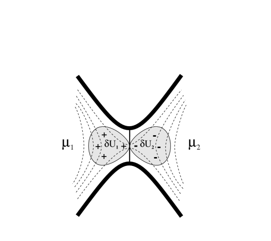
Figure 3: Charge dipole across a saddle point constriction. $\mu_{1}=eV_{1}$ and $\mu_{2}=eV_{2}$ are the potentials of the contacts, $\delta U_{1}$ and $\delta U_{2}$ are local potentials. The dashed lines are the equipotential lines of the equilibrium potential. After TCMB .

8 Transition from Capacitive to Inductive Response

The following example TCMB provides an instructive application of the ac-conduc- tance formula Eq. (43). Consider the transmission through a narrow opening shown in Fig. 3. Carrier motion is in two dimension through a potential $U(x,y)$ which has the form a saddle with a height $U_{0}$. The conductance (transmission) through such a narrow opening (a quantum point contact) has been widely studied and is found to rise step-like Wees as a function of the potential $U_{0}$ with plateaus at values $G=(2e^{2}/h)N$ corresponding to perfect transmission of $N$ spin degenerate channels. Here we are interested in the emittance $E$ as a function of $U_{0}$. We consider the case that $U_{0}$ is so large that transmission is completely blocked and then lower $U_{0}$ such that the probability of transmission probability $T$ gradually increases from $0$ to $1$.

We introduce two regions $\Omega_{1}$ and $\Omega_{2}$ to the left and the right of the barrier, respectively. Instead of the local partial density of states we consider the partial density of states integrated over the respective volumes $\Omega_{1}$ and $\Omega_{2}$. Thus we introduce $D_{\alpha k\beta}=\int_{\Omega_{k}}dxdy\nu(\alpha,x,y,\beta)$. We furthermore introduce the total density of states $D$ of the two regions. We assume that the potential has left-right symmetry and consequently the density of states in the regions $\Omega_{1}$ and $\Omega_{2}$ are $D_{1}=D_{2}=D/2$. Ref. TCMB evaluates the partial densities of states semiclassically. We find that carriers incident from contact $1$ and transmitted into contact $2$ give rise to a partial densities of states in region $1$ given by $D_{211}=TD_{1}/2$. To determine $D_{212}$, we note that in the semiclassical limit considered here, there are no states in $\Omega_{1}$ associated with scattering from contact $2$ back to contact $2$, hence it holds $D_{212}=0$. With similar arguments one finds for the semi-classical PDOS

$$D_{\alpha k\beta}=D_{k}\left(T/2+\delta_{\alpha\beta}(R\>\delta_{\alpha k}-T/2)\>\right)\;\;,\;\;\;{\rm if}\;\;\alpha,\beta\neq 3\;\;.$$ (44)

From Eq. (44) we obtain for the emissivity into contact $1$ from region $1$ and injectivity from contact $1$ into region $1$, $D^{e}_{11}=D^{i}_{11}=(1/4)(1+R)D$ and and obtain for the emissivity into contact $1$ from region $2$ and the injectivity into region $1$ from contact $2$, $D^{e}_{12}=D^{i}_{12}=(1/4)TD$. Instead of the full Poisson equation the effective interaction TCMB ; BU1 ; CURACAO is determined with the help of a geometrical capacitance $C$. For a detailed discussion we have to refer the reader to Refs. TCMB ; CURACAO . Due to charge conservation we have $E\equiv E_{11}=E_{22}=-E_{12}=-E_{21}$ with

$$E=(RC_{\mu}-DT^{2}/4)$$ (45)

Here $C_{\mu}^{-1}=R^{-1}(C^{-1}+(e^{2}D/4)^{-1})$ is the effective capacitance of the contact. It is proportional to the reflection probability and proportional to the series capacitance of the geometrical capacitance $C$ and the ”quantum capacitance” $e^{2}D$. If the contact is completely closed we have $R=1,T=0$ and the emittance is completely determined by the capacitance $C_{\mu}$. If the channel is completely open we have $R=0,T=1$ and the emittance is $E=-D/4$. It is negative indicating that for a completely open channel the ac-response is now not capacitive but inductive. Thus there is a voltage $U_{0}$ for which the emittance vanishes. For a simple saddle point potential the behavior of the capacitance and emittance is illustrated in Fig. 4. The dotted line shows the conductance, the dashed line is the capacitance $C_{\mu}$ and the full line is the emittance as a function of the saddle point potential $U_{0}$. The emittance is capacitive (positive) for a nearly closed contact and changes sign as the transmission probability increases from near $0$ to $1$. The emittance shows additional structure associated with the successive opening of further quantum channels.

A similar transition from capacitive to inductive behavior is found in the emittance of a mesoscopic wire: Guo and coworkers Guo investigate the emittance of a wire as a function of impurity concentration. A ballistic wire with no impurities has an inductive response, a disordered metallic diffusive wire has a capacitive response. Experiments on ac-transport in mesoscopic structures are challenging and we can mention here only the work by Pieper and Price pp on the ac-conductance of an Aharonov-Bohm ring and the recent work by Desrat et al. desrat on the low-frequency impedance of quantized Hall conductors.

Our simple example demonstrates the difficulty in associating a time with a result obtained by analyzing a stationary (or as here) a quasi-stationary scattering problem. The emittance divided by the conductance quantum $e^{2}/h$ has the dimension of a time. (In the non-interacting limit $e^{2}/C<<4/D$ we have Mikh $E/(e^{2}/h)=(R-T)\tau_{D}/4$ where $\tau_{D}$ is the dwell time in the two regions $\Omega_{1}$ and $\Omega_{2}$). But since this ”time” changes sign such an interpretation is not appropriate. Furthermore, in electrical problems the natural ”times” are $RC$-times if the low frequency dynamics is capacitive or an $R/L$-time if it is inductive. The fact that we describe here a crossover from capacitive to an inductive-like behavior demonstrates that neither of these two time-scales can adequately describe the dynamics.

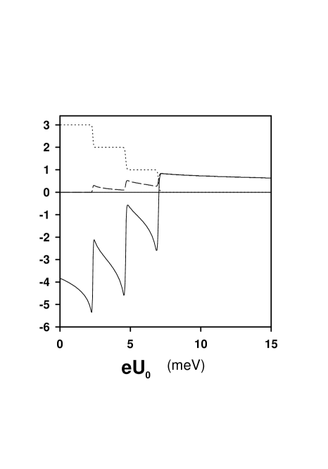
Figure 4: Conductance of the saddle point constriction (dotted line) in units of $2e^{2}/h$, capacitance and emittance (dashed and full curve) as a function of the height of the saddle point potential $U_{0}$. In the range of voltages shown three quantum channels are opened. After TCMB .

9 Partial Density of States Matrix

Thus far the main aim of our discussion has been to illustrate the concept of partial densities of states with a number of simple examples. We now would like to point to some important extensions of this concept.

Quantum mechanics is a theory of probability amplitudes. We can thus suppose that our initial state is a scattering experiment which is described by a superposition $\Psi(y)=a_{\beta}\Psi_{\beta}(y)+a_{\gamma}\Psi_{\gamma}(y)$. Here $\Psi_{\beta}$ and $\Psi_{\gamma}$ are two scattering states describing particles incident in channel $\beta$ and in channel $\gamma$ with amplitudes $a_{\beta}$ and $a_{\gamma}$. Often such superpositions are eliminated since we can assume that each incident amplitude carries its own phase $\phi_{\beta}$ and $\phi_{\gamma}$. We suppose that $a_{\beta}=|a_{\beta}|^{1/2}exp(i\phi_{\beta})$ and $a_{\gamma}=|a_{\gamma}|^{1/2}exp(i\phi_{\gamma})$ and that these phases are random and uncorrelated. Thus if an average over many scattering experiments is taken we have $<e^{i\phi_{\beta}}e^{-i\phi_{\gamma}}>=\delta_{\beta\gamma}$ and consequently we find that $<|\Psi(y)|^{2}>=|a_{\beta}|^{2}|\Psi_{\beta}|^{2}+|a_{\gamma}|^{2}|\Psi_{\gamma}|^{2}$ is the sum of scattering events in the different quantum channels. However, as soon as we are interested in quantities which depend to forth (or higher order) on the amplitudes then even after averaging over the random phases of the incident waves we find that scattering processes which involve two (or more) incident waves matter. For instance consider $<|\Psi(y)|^{2}|\Psi(y^{\prime})|^{2}>-<|\Psi(y)|^{2}><|\Psi(y^{\prime})|^{2}>$ which is determined by $|a_{\beta}|^{2}|a_{\gamma}|^{2}\Psi_{\beta}^{*}(y)\Psi_{\gamma}(y)\Psi_{\beta}(y^{\prime})\Psi_{\gamma}^{*}(y^{\prime})+h.c.$. This expression describes a correlation of the particle density at the points $y$ and $y^{\prime}$. Obviously for such higher order correlations superpositions are very important even if we associate a random phase with each incident scattering states and take an average over these phases.

We can relate such density fluctuations to functional derivatives of scattering matrix expressions. To describe density fluctuations of scattering processes with an incident carrier stream from channel $\beta$ and $\gamma$ we consider

$$\nu(\alpha,y,\beta,\gamma)=-\frac{1}{4\pi i}\left(S_{\alpha\beta}^{\dagger}\frac{\delta S_{\alpha\gamma}}{\delta V(y)}-\frac{\delta S_{\alpha\beta}^{\dagger}}{\delta V(y)}S_{\alpha\gamma}\right)\;\;$$ (46)

Note that two different scattering matrices enter into this expression. The connection to the scattering states is determined by the relation

$$\sum_{\alpha}\nu(\alpha,y,\beta,\gamma)=(1/h)(v_{\beta}v_{\gamma})^{-1/2}\Psi_{\beta}^{*}(y)\Psi_{\gamma}(y)\;\;$$ (47)

Here $v_{\beta}$ and $v_{\gamma}$ are the (asymptotic) velocities of the carriers in the scattering channels ${\beta}$ and ${\gamma}$ far away from the scattering region. Eq. (47) was given in Ref. math and a detailed derivation of this relation is presented in ankara .

The expressions $\nu(\alpha,y,\beta,\gamma)$ can be viewed as the off-diagonal elements of a partial density of states matrix. In Eq. (47) we take the sum over out-going channels. The resulting matrix is the local density of states matrix. Using Eq. (46) in Eq. (47) we find,

$$\nu(y,\beta,\gamma)\equiv\sum_{\alpha}\nu(\alpha,y,\beta,\gamma)=-\frac{1}{2\pi i}\sum_{\alpha}\left(S_{\alpha\beta}^{\dagger}\frac{\delta S_{\alpha\gamma}}{\delta V(y)}\right)\;\;$$ (48)

where we have taken into account that the scattering matrix is unitary.

Let us now consider the total density of states matrix. The fluctuations of interest are then the total particle number fluctuations in the scattering region ${\Omega}$, $D(\beta,\gamma)=\int_{\Omega}dy\nu(y,\beta,\gamma)$. Furthermore, if the volume of integration is sufficiently large, we can, in WKB approximation, replace the functional derivative with respect to $V$ with a derivative with respect to energy. The matrix which governs the fluctuations in the particle number in the scattering region then becomes,

$$D(\beta,\gamma)=\frac{1}{2\pi i}\sum_{\alpha}\left(S_{\alpha\beta}^{\dagger}\frac{dS_{\alpha\gamma}}{dE}\right)\;\;$$ (49)

Eq. (49) is the Wigner-Smith delay time matrix Smith . We have earlier emphasized that the appearance of the energy derivative is a consequence of approximations (here the fact that we consider the WKB limit). We also mention that strictly speaking, here we do not consider a ”delay”. We do not compare with a reference scattering problem (a free motion) as is typically done in nuclear scattering problems. Eq. (49) determines a total time or absolute time and we should more appropriately call it the absolute time matrix instead of the delay time matrix.

The partial density of states matrix has been used in Ref. math to obtain the second order in frequency term of the ac-conductance (see Eq. (42)). Ref. plb investigated the current induced into a nearby gate due to charge fluctuations in quantum point contacts and chaotic cavities. More recently, the charge fluctuations in two nearby mesoscopic conductors was treated with this approach and the effect of quantum dephasing due to charge fluctuations was calculated within this approach mbam ; ankara . The results can be compared with other theoretical works levinson and with experiments buks1 .

The Wigner-Smith delay time matrix has received wider attention. In recent years the focus has been on the calculation of the entire distribution function of delay times Sommers for structures whose dynamic is in the classical limit chaotic (chaotic cavities). Predominantly structures have been investigated in which carrier propagation is an allowed energy region.

We conclude by briefly discussing the Wigner-Smith matrix for a tunnel barrier. For a symmetric barrier with transmission and reflection probability $T$ and $R$ the scattering matrix has elements $S_{11}=S_{22}=-i\sqrt{R}\exp(i\phi)$, and $S_{21}=S_{12}=\sqrt{T}\exp(i\phi)$ where $\phi$ is the phase accumulated during a reflection or transmission process. Thus the elements of the Wigner-Smith delay time matrix Eq. (49) are

$${\cal D}_{11}={\cal D}_{22}=\frac{1}{2\pi}\frac{d\phi_{n}}{dE},\,\,{\cal D}_{12}={\cal D}_{21}=\frac{1}{4\pi}\frac{1}{\sqrt{R_{n}T_{n}}}\frac{dT_{n}}{dE}.$$ (50)

To be specific consider now the case of a tunnel barrier. In the WKB limit we have $R\approx 1$ and $T=exp(-2S/\hbar)$ with $S=\int dy\sqrt{2m}\sqrt{V(y)-E}$ where the integral extends from one turning point to the other. We have $d\phi/dE=0$ and using the expression $\tau_{T}=m\int dy(\sqrt{2m}\sqrt{V(y)-E})^{-1}$ for the traversal time of tunneling gives $dT/dE=(2\tau_{T}/\hbar)T$. Consequently, the diagonal elements of the Wigner-Smith matrix vanish and the non-diagonal elements are

$${\cal D}_{12}={\cal D}_{21}=\frac{\tau_{T}}{2\pi\hbar}\sqrt{T}.$$ (51)

Thus while the the average density inside the barrier vanishes (the trace of the Wigner-Smith matrix is zero) the off-diagonal elements are non-zero and indicate that the fluctuations of the charge will in general be non-vanishing even deep inside the classically forbidden region.

The discussion of this section rests admittedly vague. While important first steps have been made to extend the notion of partial density of states to treat fluctuations, our discussion shows that even at the conceptual level, there is clearly room for more research.

Another development which could be discussed here is a theory of quantum pumping in small systems. In quantum pumping one is interested in the current generated as two parameters (like gate voltages, magnetic fluxes) which modulate the system are varyed sinusoidally but out of phase. Brouwer BR1 , Avron et al. Avron , Shutenko et al. alein and Polianski and Brouwer BR2 develop a theory which is based on the modulation of the partial densities of states discussed here.

10 Discussion

The Larmor clock and its close relatives have become one of the most widely investigated approaches mainly in order to understand the question: ”How long does a particle traveling through a classically forbidden region (a tunnel barrier) interact with this region?”. We have already in the previous sections pointed out that there is no consensus in the interpretation even of this simple clock. Regardless of these difficulties the investigation of the Larmor clock has been helpful in understanding a number of transport problems: In particular we have discussed a hierarchy of density of states as they occur in open multiprobe mesoscopic conductors. These density of states are directly related to local Larmor times. We have shown that a small absorption or a small emission of particles can be described with these densities (or in terms of the Larmor times). We have shown that the transmission probabilities through weakly coupled contacts like the STM is related to these densities. We have shown that a weakly coupled voltage probe, describing inelastic scattering or a dephasing process can be treated in terms of these densities. We have also pointed out that the ac-conductance of a mesoscopic conductor at small frequencies can be expressed with the help of these densities. Furthermore, we have indicated that it is useful to consider also the off-diagonal elements of a partial density of states matrix since this permits a description of fluctuation processes. Thus there is no question that the investigation of the Larmor clock has been a very fruitful and important enterprise.

References

- (1) A. I. Baz’, Sov. J. Nuc. Phys. 4, 182 (1967); 5, 161 (1967).
- (2) V. F. Rybachenko, Sov. J. Nucl. Phys. 5, 635 (1967).
- (3) M. Büttiker, Phys. Rev. B 27, 6178 (1983).
- (4) C. R. Leavens and G. C. Aers, Solid State Commun. 63, 1107 (1989).
- (5) C. R. Leavens and G. C. Aers Phys. Rev. B 40, 5387-5400 (1989).
- (6) M. Büttiker, J. Phys.: Condensed Matter 5, 9361 (1993).
- (7) M. Büttiker, H. Thomas, and A. Prêtre, Z. Phys. B 94, 133 (1994).
- (8) M. Büttiker, A. Prêtre and H. Thomas, Phys. Rev. Lett. 70, 4114 (1993); M. Büttiker, H. Thomas, and A. Prêtre, Phys. Lett. A 180, 364 (1993).
- (9) V. Gasparian, T. Christen, and M. Büttiker, Phys. Rev. A 54, 4022 (1996).
- (10) T. Gramespacher and M. Buttiker, Phys. Rev. B 56, 13026-13034 (1997); Phys. Rev. B 60, 2375-2390 (1999); Phys. Rev. B 61, 8125-8132 (2000).
- (11) R. Dashen, S. Ma, and H. J. Bernstein, Phys. Rev. 187, 345 (1969).
- (12) Y. Avishai and Y. B. Band, Phys. Rev. B 32, 2674 (1985).
- (13) G. Iannaccone, Phys. Rev. B 51, 4727 (1995).
- (14) G. Iannaccone and B. Pellegrini, Phys. Rev. B 53, 2020 (1996).
- (15) M. Büttiker and R. Landauer, Phys. Rev. Lett. 49, 1739 (1982); Physica Scripta 32, 429-434, (1985).
- (16) D. Sokolovski and L. M. Baskin Phys. Rev. A 36, 4604-4611 (1987); H. A. Fertig, Phys. Rev. B 47, 1346-1358 (1993).
- (17) V. Gasparian, M. Ortuno, J. Ruiz, and E. Cuevas Phys. Rev. Lett. 75, 2312 (1995); Y. Japha and G. Kurizki, Phys. Rev. A 60, 1811 (1999).
- (18) A. M. Steinberg, Phys. Rev. Lett. 74, 2405 (1995).
- (19) S. Brouard, R. Sala, J. G. Muga, Phys. Rev. A 49 4312 (1994).
- (20) X. Zhao, J. Phys. Cond. Matter, 12, 4053 (2000).
- (21) M. Büttiker, in ”Electronic Properties of Multilayers and low Dimensional Semiconductors”, edited by J. M. Chamberlain, L. Eaves, and J. C. Portal, (Plenum, New York, 1990). p. 297-315.
- (22) S. A. Ramakrishna and N. Kumar, Phys. Rev. B 61, 3163 (2000).
- (23) C.W.J. Beenakker, cond-mat/0009061
- (24) P. W. Brouwer, S. A. van Langen, K. M. Frahm, M. Büttiker, and C. W. J. Beenakker, Phys. Rev. Lett. 79, 914 (1997).
- (25) G. Binnig and H. Rohrer, Helv. Phys. Acta 55, 726 (1982); J. Tersoff and D. R. Hamann, Phys. Rev. B 31, 805 (1985).
- (26) M. Büttiker, IBM J. Res. Develop. 32, 63 (1988).
- (27) P. W. Brouwer and C. W. J. Beenakker, Phys. Rev. B 55, 4695 (1997).
- (28) T. P. Pareek, Sandeep K. Joshi, A. M. Jayannavar, Phys. Rev. B 57, 8809 (1998).
- (29) M. Büttiker, in ”Analogies in Optics and Micro-Electronics”, edited by W. van Haeringen and D. Lenstra, Kluwer Academic Publishers, (Dordrecht-Boston-London, 1990). p. 185-202.
- (30) T. Christen and M. Büttiker, Phys. Rev. Lett. 77, 143 (1996).
- (31) B. J. van Wees et al., Phys. Rev. Lett. 60, 848 (1988); D. A. Wharam et al., J. Phys. C: Solid State Phys. 21, L209 (1988).
- (32) M. Büttiker and T. Christen, in ”Mesoscopic Electron Transport”, NATO Advanced Study Institute, Series E: Applied Science, edited by L. L. Sohn, L. P. Kouwenhoven and G. Schoen, (Kluwer Academic Publishers, Dordrecht, 1997). Vol. 345. p. 259. cond-mat/9610025
- (33) Tiago De Jesus, Hong Guo, and Jian Wang, Phys. Rev. B 62, 10774 (2000).
- (34) J. P. Pieper and and J. C. Price, Phys. Rev. Lett. 72, 3586 (1994).
- (35) W. Desrat, D. K. Maude, L. B. Rigal, M. Potemski, J. C. Portal, L. Eaves, M. Henini, Z. R. Wasilewski, A. Toropov, G. Hill and M. A. Pate, Phys. Rev. B 62 12990 (2000).
- (36) S. A. Mikhailov and V. A. Volkov, JETP Lett. 61, 524 (1995).
- (37) M. Büttiker, J. Math. Phys., 37, 4793 (1996).
- (38) M. Büttiker, in ”Quantum Mesoscopic Phenomena and Mesoscopic Devices”, edited by I. O. Kulik and R. Ellialtioglu, (Kluwer, Academic Publishers, Dordrecht, 2000). Vol. 559, p. 211. cond-mat/9911188
- (39) F. T. Smith, Phys. Rev. 118 349 (1960).
- (40) M. H. Pedersen, S. A. van Langen and M. Büttiker, Phys. Rev. B 57, 1838 (1998).
- (41) M. Büttiker and A. M. Martin, Phys. Rev. B 61, 2737 (2000).
- (42) Y. B. Levinson, Europhys. Lett. 39, 299 (1997); L. Stodolsky, Phys. Lett. B 459, 193 (1999).
- (43) E. Buks, R. Schuster, M. Heiblum, D. Mahalu and V. Umansky, Nature 391, 871 (1998); D. Sprinzak, E. Buks, M. Heiblum and H. Shtrikman, Phys. Rev. Lett. 84, 5820 (2000).
- (44) Y. V. Fyodorov and H. J. Sommers, Phys. Rev. Lett. 76, 4709 (1996); V. A. Gopar, P. A. Mello, and M. Büttiker, Phys. Rev. Lett. 77, 3005 (1996); P. W. Brouwer, K. M. Frahm, and C. W. J. Beenakker, Phys. Rev. Lett. 78, 4737 (1997); C. Texier and A. Comtet, ibid.82, 4220 (1999).
- (45) P.W. Brouwer, Phys. Rev. B 58, R10 135 (1998).
- (46) J. E. Avron, A. Elgart, G. M. Graf, and L. Sadun, Phys. Rev. B 62, R10618 (2000).
- (47) T. A. Shutenko, I. L. Aleiner, B. L. Altshuler, Phys. Rev. B61, 10366 (2000).
- (48) M. L. Polianski, P. W. Brouwer, cond-mat/0102159