Enhanced Estimation of a Noisy Quantum Channel Using Entanglement

Abstract

We discuss the estimation of channel parameters for a noisy quantum channel – the so-called Pauli channel – using finite resources. It turns out that prior entanglement considerably enhances the fidelity of the estimation when we compare it to an estimation scheme based on separable quantum states.

I Introduction

In the last few years, the field of quantum information processing has made enormous progress. It has been shown that the laws of quantum mechanics open completely new ways of communication and computation [1]. This progress has mainly been driven by understanding more and more about the physics of entanglement. The corresponding nonclassical correlations are central to completely new applications like quantum cryptography using entangled systems [2], teleportation [3] and dense coding [4]. These are all examples of superior information transmission with quantum mechanical means.

Consequently, much work has been done toward the understanding of quantum communication channels. In principle a quantum channel is simply a transmission line between a sender, say Alice, and a receiver, say Bob, that allows them to transfer quantum systems. The noiseless channel leaves the quantum states of the transmitted systems intact. In other words, such a channel is completely isolated from any environment. This is certainly a strong idealization. More realistic is the noisy quantum channel that takes into account the interaction of the sent system with an environment: the corresponding quantum state decoheres. In effect this process can be described by a superoperator $C$ which in general maps Alice’s pure state $|\psi\rangle\langle\psi|$ on a density operator $\hat{\rho}=C(|\psi\rangle\langle\psi|)$ on Bob’s side [5].

The prominent topics of research in the field of quantum channel theory are to understand the notion of capacity of a quantum channel and to understand the role played by entanglement. The proof [6] of the quantum analog of Shannon’s noiseless coding theorem [7] was a milestone in this field indicating that a quantum theory of information transmission is possible in parallel to its classical counterpart. Consequently, much work then concentrated on the concept of capacity for a general noisy quantum channel [8, 9]. Hence these investigations aim at quantifying the maximum rate at which information can be sent through a noisy quantum channel: in analogy to the noisy-channel coding theorem of Shannon [7]. Moreover, it was shown [8] that entanglement can be used as a resource to quantify the noise of a quantum channel.

However, since a quantum channel can carry classical as well as quantum information, several different capacities can be defined [8, 9]. In particular, it is well-known that prior entanglement can enhance the capacity of quantum channels to transmit classical information [4, 10]. It is therefore justified to consider entanglement as a fruitful resource which has no classical analogue [11].

In the present paper we shall discuss a different application of entanglement in the field of quantum channels. Let us suppose that Alice and Bob are connected by a specific noisy channel. Both parties know about the fundamental errors imposed by the noise but they have no information about the corresponding error strengths. Hence, before Alice and Bob use the channel for communication they would like to estimate the corresponding error rates. Then they can, for example, decide on a suitable error correction scheme [12] or choose a suitable encoding for their information [13]. In the remainder of the paper we will show that prior entanglement substantially increases the average reliability of their estimation.

II The Pauli Channel

The channel that we will investigate in this paper is the so called Pauli channel $C$ which causes single qubit errors. These single qubit errors can be fully classified by the Pauli spin operators $\hat{\sigma}_{1}=|0\rangle\langle 1|+|1\rangle\langle 0|$, $\hat{\sigma}_{2}=i(|1\rangle\langle 0|-|0\rangle\langle 1|)$ and $\hat{\sigma}_{3}=|0\rangle\langle 0|-|1\rangle\langle 1|$ in the computational basis defined by $|0\rangle$ and $|1\rangle$. The application of the unitary operators $\hat{\sigma}_{i}$ leads to a fundamental rotation of a qubit state $|q\rangle=c_{0}|0\rangle+c_{1}|1\rangle$ with coefficients $c_{i}$. The bit flip error is given by $\hat{\sigma}_{1}$, that is, $\hat{\sigma}_{1}|q\rangle=c_{0}|1\rangle+c_{1}|0\rangle$. It exchanges the two basis states. The phase-flip error $\hat{\sigma}_{3}|q\rangle=c_{0}|0\rangle-c_{1}|1\rangle$ changes the sign of $c_{1}$ in any coherent superposition of the basis states. Finally $\hat{\sigma}_{2}$ generates a combination of bit and phase flip.

In a Pauli channel each of the three errors can occur with a certain probability $p_{i}$ so that the superoperator reads

$$C(\hat{\rho})=\sum_{i=1}^{4}p_{i}\hat{\sigma}_{i}\hat{\rho}\hat{\sigma}_{i}^{\dagger}$$ (1)

with $\hat{\sigma}_{4}=\hat{1}$ and with probability $p_{4}=1-p_{1}-p_{2}-p_{3}$ that the density operator remains unchanged. Hence the Pauli channel is completely characterized by a parameter vector $\vec{p}=(p_{1},p_{2},p_{3})^{T}$. Thus the action of the channel on the general density operator

$$\hat{\rho}(\vec{s})=\frac{1}{2}\left(\hat{1}+\sum_{i=1}^{3}s_{i}\hat{\sigma}_{i}\right)$$ (2)

defined by the Bloch vector $\vec{s}=(s_{1},s_{2},s_{3})^{T}$ with $s_{i}\in\mathbb{R}$ and $|\vec{s}|\leq 1$ can be described by the basic transformations

$$C(\hat{\sigma}_{1}) = \left[1-2(p_{2}+p_{3})\right]\hat{\sigma}_{1}$$ (3)

$$C(\hat{\sigma}_{2}) = \left[1-2(p_{1}+p_{3})\right]\hat{\sigma}_{2}$$ (4)

$$C(\hat{\sigma}_{3}) = \left[1-2(p_{1}+p_{2})\right]\hat{\sigma}_{3}$$ (5)

and $C(\hat{1})=\hat{1}$. Our aim is to estimate the parameters $p_{i}$ from a finite amount of measurement results. Hence the general scenario is the following: Alice prepares qubits in well-known reference states and sends them to Bob through the channel to be estimated. Bob knows those reference states and performs suited measurements on the qubits he has received. The statistics of his measurement results will then allow him to estimate the parameters $p_{i}$.

III Channel Estimation

First, we consider the case – also depicted in Fig. 1a – that Alice sends single qubits through the channel. In order to determine $\vec{p}$ Alice has to prepare three well-defined reference states. For each of the states Bob then measures one operator so that at the end Bob has measured three independent operators.

The natural choice is that Alice prepares three pure states (a) $\hat{\rho}_{1}=\hat{\rho}(\vec{s}=(1,0,0)^{T})$, (b) $\hat{\rho}_{2}=\hat{\rho}(\vec{s}=(0,1,0)^{T})$, (c) $\hat{\rho}_{3}=\hat{\rho}(\vec{s}=(0,0,1)^{T})$ and Bob measures the operators (a) $\hat{\sigma}_{1}$, (b) $\hat{\sigma}_{2}$ and (c) $\hat{\sigma}_{3}$ [14]. The corresponding expectation values $\langle\hat{\sigma}_{i}\rangle=1-2P_{i}$ depend on the probability $P_{i}$ to measure the eigenvalue $-1$ (spin down) in each case. With the help of Eqs. (2) and (3) we immediately find that the parameter vector

$$\vec{p}=\frac{1}{2}\left(\begin{array}[]{c}P_{3}-P_{1}+P_{2}\\ P_{1}-P_{2}+P_{3}\\ P_{2}-P_{3}+P_{1}\end{array}\right)$$ (6)

can be calculated from the measured probabilities $P_{i}$.

If only finite resources are available Bob just finds frequencies instead of probabilities. Using $M$ qubits for each of the three input states and the corresponding measurements yields the estimated parameters

$$\vec{p}^{\;est}=\frac{1}{2M}\left(\begin{array}[]{c}i_{3}-i_{1}+i_{2}\\ i_{1}-i_{2}+i_{3}\\ i_{2}-i_{3}+i_{1}\end{array}\right)$$ (7)

if $i_{j}$ results “$-1$” are recorded for the measurement of $\hat{\sigma}_{j}$. The reason why we choose the same number of $M$ qubits for each of these measurements is that we assume complete ignorance about the probabilities $p_{i}$.

As the measure of estimation quality we use a standard statistical measure, namely the quadratic deviation $\sum_{j=1}^{3}(p_{j}-p_{j}^{est})^{2}$ which describes the error of the estimation. With this choice of cost function we find the average error

$$\bar{f}(M,\vec{p}) = \sum_{i_{1}=0}^{M}\sum_{i_{2}=0}^{M}\sum_{i_{3}=0}^{M}{M\choose i_{1}}{M\choose i_{2}}{M\choose i_{3}}(p_{2}+p_{3})^{i_{1}}$$ (8)

$$\times (1-p_{2}-p_{3})^{M-i_{1}}(p_{1}+p_{3})^{i_{2}}(1-p_{1}-p_{3})^{M-i_{2}}$$ (9)

$$\times (p_{1}+p_{2})^{i_{3}}(1-p_{1}-p_{2})^{M-i_{3}}\sum_{j=1}^{3}(p_{j}-p_{j}^{est})^{2}$$ (10)

$$= \frac{3}{2M}\left[p_{1}(1-p_{1})+p_{2}(1-p_{2})+p_{3}(1-p_{3})\right.$$ (11)

$$- \left.p_{1}p_{2}-p_{2}p_{3}-p_{1}p_{3}\right]$$ (12)

averaged over all possible experimental outcomes.

Up to now we have only considered the case that Alice sends $N=3M$ single unentangled qubits through the Pauli channel. However, one could also think of using entangled qubit pairs (ebits) to estimate the channel parameters. For this purpose we consider the following second scenario which is also shown in Fig. 1b: Alice and Bob share an ebit prepared in a $|\psi^{-}\rangle=1/\sqrt{2}(|0\rangle|1\rangle-|1\rangle|0\rangle)$ Bell state. Alice sends her qubit through the Pauli channel whereas Bob simply keeps his qubit. The channel causes the transformation

$$C(|\psi^{-}\rangle\langle\psi^{-}|) = p_{1}|\phi^{-}\rangle\langle\phi^{-}|+p_{2}|\phi^{+}\rangle\langle\phi^{+}|+p_{3}|\psi^{+}\rangle\langle\psi^{+}|$$ (13)

$$+ (1-p_{1}-p_{2}-p_{3})|\psi^{-}\rangle\langle\psi^{-}|.$$ (14)

The Pauli channel transforms the initial $|\psi^{-}\rangle$ state into a mixture of all four Bell states $|\phi^{\pm}\rangle=1/\sqrt{2}(|0\rangle|0\rangle\pm|1\rangle|1\rangle)$, $|\psi^{\pm}\rangle=1/\sqrt{2}(|0\rangle|1\rangle\pm|1\rangle|0\rangle)$ where each Bell state is generated by exactly one of the possible single qubit errors $\hat{\sigma}_{j}$. Bob now performs a Bell measurement in which he finds each Bell state with probability

$$P_{|\phi^{-}\rangle}= p_{1} \qquad P_{|\phi^{+}\rangle}=p_{2}\qquad P_{|\psi^{+}\rangle}=p_{3}$$ (15)

$$P_{|\psi^{-}\rangle} =1-p_{1}-p_{2}-p_{3}.$$ (16)

Note that Alice and Bob can only use the same qubit resources as before. That is, if they have used $N$ single qubits before they can now generate $N^{\prime}=N/2$ ebits in the reference state $|\psi^{-}\rangle$. Consequently Bob gets only half as many measurement results as before: he finds four values $i_{1}$, $i_{2}$, $i_{3}$ and $i_{4}$ with $\sum_{j=1}^{4}i_{j}=N^{\prime}$ for the number of occurrences of the Bell states $|\phi^{-}\rangle$, $|\phi^{+}\rangle$, $|\psi^{+}\rangle$ and $|\psi^{-}\rangle$. From these four values he can calculate the estimated probabilities

$$p_{1}^{est}=\frac{i_{1}}{N^{\prime}} p_{2}^{est}=\frac{i_{2}}{N^{\prime}}\qquad p_{3}^{est}=\frac{i_{3}}{N^{\prime}}$$ (17)

that fully characterize the Pauli channel. The average error for the estimation scheme with entangled qubits then reads

$$\bar{g}(N^{\prime},\vec{p}) = \sum_{i_{1}+i_{2}+i_{3}+i_{4}=N^{\prime}}\frac{N^{\prime}!}{i_{1}!i_{2}!i_{3}!i_{4}!}$$ (18)

$$\times p_{1}^{i_{1}}p_{2}^{i_{2}}p_{3}^{i_{3}}(1-p_{1}-p_{2}-p_{3})^{i_{4}}\sum_{j=1}^{3}(p_{j}-p_{j}^{est})^{2}$$ (19)

$$= \sum_{i_{1}=0}^{N^{\prime}}\sum_{i_{2}=0}^{N^{\prime}-i_{1}}\sum_{i_{3}=0}^{N^{\prime}-i_{1}-i_{2}}\frac{N^{\prime}!}{i_{1}!i_{2}!i_{3}!(N^{\prime}-i_{1}-i_{2}-i_{3})!}$$ (20)

$$\times p_{1}^{i_{1}}p_{2}^{i_{2}}p_{3}^{i_{3}}(1-p_{1}-p_{2}-p_{3})^{N^{\prime}-i_{1}-i_{2}-i_{3}}$$ (21)

$$\times \sum_{j=1}^{3}(p_{j}-\frac{i_{j}}{N^{\prime}})^{2}$$ (22)

$$= \frac{1}{N^{\prime}}\left[p_{1}(1-p_{1})+p_{2}(1-p_{2})+p_{3}(1-p_{3})\right].$$ (23)

We can now compare the average errors, Eqs. (6) and (10), for both estimation schemes. As emphasized above for a fair comparison we have to consider the same number $N=2N^{\prime}=3M$ of available qubits for both schemes. We find that the difference

$$\Delta(N,\vec{p}) = \bar{f}(M=N/3,\vec{p})-\bar{g}(N^{\prime}=N/2,\vec{p})$$ (24)

$$= \frac{1}{2N}\left[5(1-p_{1}-p_{2}-p_{3})(p_{1}+p_{2}+p_{3})\right.$$ (25)

$$+ \left.p_{1}p_{2}+p_{1}p_{3}+p_{2}p_{3}\right]\geq 0$$ (26)

is non-negative for all possible parameter values $\vec{p}$. This clearly shows that we indeed get an enhancement of the estimation quality due to the use of entangled qubit pairs. This enhancement is illustrated in Fig. 2 for the case $p_{2}=0$ which already shows the typical features of $\Delta$. We see that $\Delta(N,\vec{p})$ is always positive except for the extremal points $\vec{p}=(0,0,0)^{T}$, $\vec{p}=(1,0,0)^{T}$ and $\vec{p}=(0,0,1)^{T}$ where $\Delta$ vanishes.

Instead of comparing the errors for the same number of available qubits one could also compare the estimation quality for the same number $K$ of channel applications. For the latter case we have $K=N^{\prime}=3M$ so that the enhancement

$$\tilde{\Delta}(K,\vec{p}) = \bar{f}(M=K/3,\vec{p})-\bar{g}(N^{\prime}=K,\vec{p})$$ (27)

$$= \frac{1}{2K}\left[7(1-p_{1}-p_{2}-p_{3})(p_{1}+p_{2}+p_{3})\right.$$ (28)

$$+ \left.5p_{1}p_{2}+5p_{1}p_{3}+5p_{2}p_{3}\right]\geq 0$$ (29)

due to entanglement is even larger.

IV Conclusion

In conclusion we have shown a new application in which entanglement serves as a superior resource for quantum information processing: In the case of the Pauli channel there is a significant improvement in the estimation of the error strengths due to the use of entangled qubits instead of separable ones. Hence entanglement allows a better characterization of the quantum channel for finite initial resources which can be counted in terms of available qubits or in terms of channel applications. In contrast to dense coding [4], where we achieve an optimal encoding of information by entanglement, we obtain an enhanced extraction of information about a quantum channel here. As a consequence this additional information about the channel can be used in practical quantum communication problems to optimize error correction schemes [12] or signal ensembles [13].

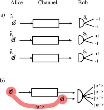
FIG. 1.: The two schemes for estimating the Pauli-channel parameters $p_{i}$ from an initial supply of $N$ qubits. In scheme a) Alice prepares single qubits in three different quantum states $\hat{\rho}_{i}$ ($M=N/3$ qubits in each state) and sends them through the quantum channel. After receiving the qubits Bob measures the operator $\hat{\sigma}_{i}$ for each qubit. Thus he finally possesses $N$ measurement results from which he estimates the parameters $p_{i}$. In scheme b) Alice and Bob share $N^{\prime}=N/2$ entangled pairs of qubits prepared in a $|\psi^{-}\rangle$ Bell state. Alice sends her qubit through the quantum channel to Bob who then performs a Bell measurement onto the qubit pairs. In this scheme Bob records only $N/2$ measurement results.

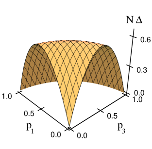
FIG. 2.: Plot of the estimation enhancement due to the use of entangled qubit pairs. For the specific example of $p_{2}=0$ we have plotted $N\Delta$, Eq. (11), versus the channel probabilities $p_{1}$ and $p_{3}$ in the allowed parameter range $0\leq p_{1}+p_{3}\leq 1$. This quantity which is independent of $N$ is always non-negative. For $p_{2}=0$ the maximum gain of $N\Delta_{max}=25/38\approx 0.66$ is reached for $p_{1}=p_{3}=5/19$. In the general case ($p_{2}\geq 0$) the maximum value of $N\Delta_{max}=75/112\approx 0.67$ is found for $p_{1}=p_{2}=p_{3}=5/28$.

- [1] For a recent review see D. Bouwmeester, A. Ekert, and A. Zeilinger (Eds.), The Physics of Quantum Information (Springer, Berlin, 2000) and the references cited therein.
- [2] A.K. Ekert, Phys. Rev. Lett. 67, 661 (1991).
- [3] C.H. Bennett, G. Brassard, C. Crepeau, R. Jozsa, A. Peres, and W.K. Wootters, Phys. Rev. Lett. 70, 1895 (1993); for more references see Ref. [1].
- [4] C.H. Bennett and S.J. Wiesner, Phys. Rev. Lett. 69, 2881 (1992).
- [5] K. Kraus, States, Effects, and Operations, Lecture Notes in Physics Vol. 190 (Springer, Berlin, 1983).
- [6] B. Schumacher, Phys. Rev. A 51, 2738 (1995).
- [7] G.E. Shannon and W. Weaver,The Mathematical Theory of Communication (University of Illinois Press, Urbana, 1949).
- [8] B. Schumacher, Phys. Rev. A 54, 2614 (1996).
- [9] B. Schumacher and M.A. Nielsen, Phys. Rev. A 54, 2629 (1996); C.H. Bennett, D.P. DiVincenzo, J.A. Smolin, and W.K. Wootters, Phys. Rev. A 54, 3824 (1996); S. Lloyd, Phys. Rev. A 55, 1613 (1997); C.H. Bennett, D.P. DiVincenzo, and J.A. Smolin, Phys. Rev. Lett. 78, 3217 (1997); B. Schumacher and M.D. Westmoreland, Phys. Rev. A 56, 131 (1997); C. Adami and N.J. Cerf, Phys. Rev. A 56, 3470 (1997); H. Barnum, M.A. Nielsen, and B. Schumacher, Phys. Rev. A 57, 4153 (1998); D.P. DiVincenzo, P.W. Shor, and J.A. Smolin, Phys. Rev. A 57, 830 (1998).
- [10] C.H. Bennett, P.W. Shor, J.A. Smolin, and A.V. Thapliyal, Phys. Rev. Lett. 83, 1459 (1999).
- [11] H.K. Lo and S. Popescu, Phys. Rev. Lett. 83, 1459 (1999).
- [12] P.W. Shor, Phys. Rev. A 52, R2493 (1995); A.R. Calderbank and P.W. Shor, Phys. Rev. A 54, 1098 (1996); R. Laflamme, C. Miquel, J.P. Paz, and W.H. Zurek, Phys. Rev. Lett. 77, 198 (1996); A.M. Steane, Phys. Rev. Lett. 77, 793 (1996); E. Knill and R. Laflamme, Phys. Rev. A 55, 900 (1997).
- [13] B. Schumacher and M.D. Westmoreland, e-print quant-ph/9912122 (1999).
- [14] The reason why this choice of prepared input states is optimal is that they are eigenstates of one of the channel error operators , cp. Eq. (3). Thus the resulting output states only depend on two instead of three channel parameters . The measurements are then designed in such a way that the variation in measured probabilities due to a change of channel parameters is maximal.