Maximizing the entanglement of two mixed qubits

Abstract

Two-qubit states occupy a large and relatively unexplored Hilbert space. Such states can be succinctly characterized by their degree of entanglement and purity. In this letter we investigate entangled mixed states and present a class of states that have the maximum amount of entanglement for a given linear entropy.

With the recent rapid developments in quantum information there has been a renewed interest in multiparticle quantum mechanics and entanglement. The properties of states between the pure, maximally-entangled, and completely mixed (separable) limits are not completely known and have not been fully characterized. The physically allowed degree of entanglement and mixture is a timely issue, given that entangled qubits are a critical resource in many quantum information applications (such as quantum computationDiVincenzo95 ; Vedral98 , quantum communicationSchumacher96 , quantum cryptographyEkert 91 ; Naik00 and teleportationBennett93 ; Bouwmeester97 ), and that entangled mixed states could be advantageous for certain quantum information situationsCleve99 .

The simplest non-trivial multiparticle system that can be investigated both theoretically and experimentally consists of two-qubits. A two-qubit system displays many of the paradoxical features of quantum mechanics such as superposition and entanglement. Extreme cases are well known and clear enough: maximally-entangled two particle states have been produced in a range of physical systems Aspect 82 ; Kwiat99 ; Turchette98 ; Turchette95 , while two-qubits have been encoded in product (non-entangled) states Braunstein99 via liquid NMR Chuang98 . Recently, however White et al. have experimentally generated polarization-entangled photons in both non-maximally entangled statesWhite99 , and general states with variable degree of mixture and entanglement White00 .

In this letter we explore theoretically the domain between pure, highly entangled states, and highly mixed, weakly entangled states. We will partially characterisepartial such two-qubit states by their purity and degree of entanglement Bennett96 . Specifically, we address the question: What is the form of maximally-entangled mixed states, that is, states with the maximum amount of entanglement for a given degree of purity? Ishizaka et al. Ishizaka00 have proposed two-qubit mixed states in which the degree of entanglement cannot be increased further by any unitary operations (the Werner stateWerner89 is one such example). A numerical exploration of the entanglement - purity plane is used to establish an upper bound for the maximum amount of entanglement possible for a given purity, and vice versa. We derive an analytical form for this class of maximally-entangled mixed states (MEMS) and show it to be optimal for the entanglement and purity measures considered.

Currently a variety of measures are known for quantifying the degree of entanglement in a bipartite system. These include the entanglement of distillationBennett96 , the relative entropy of entanglementVedral98 , but the canonical measure of entanglement is called the entanglement of formation (EOF) Bennett96 and for an arbitrary two-qubit system is given byCoffman99

$$E_{F}(\hat{\rho})=h\left(\frac{1+\sqrt{1-\tau}}{2}\right),$$ (1)

where $h(x)=-x\log_{2}(x)-(1-x)\log_{2}(1-x)$ is Shannon’s entropy function and $\tau$, the “tangle” Coffman99 (“concurrence” squared) is given by

$$\tau={\cal C}^{2}=\left[\max\{\lambda_{1}-\lambda_{2}-\lambda_{3}-\lambda_{4},0\}\right]^{2},$$ (2)

Here the $\lambda$’s are the square roots of the eigenvalues, in decreasing order, of the matrix, $\hat{\rho}\tilde{\hat{\rho}}=\hat{\rho}\;\sigma_{y}^{A}\otimes\sigma_{y}^{B}\hat{\rho}^{*}\sigma_{y}^{A}\otimes\sigma_{y}^{B}$, where $\hat{\rho}^{*}$ denotes the complex conjugation of $\hat{\rho}$ in the computational basis $\{|00\rangle,|01\rangle,|10\rangle,|11\rangle\}$, and is an anti-unitary operation. Since the entanglement of formation $E_{F}$ is a strictly monotonic function of $\tau$, the maximum of $\tau$ corresponds to the maximum of $E_{F}$. Thus in this letter we use the tangle directly as our measure of entanglement. For a maximally-entangled pure state $\tau=1$, while for a unentangled state $\tau=0$.

There exist for the degree of mixture of a state a number of measures. These include the von Neumann entropy of a state, given by $\rm{S}=-\rm{Tr}[\hat{\rho}\rm{ln}\hat{\rho}]$ vonNeumann55 , and the purity ${\rm Tr}[\hat{\rho}^{2}]$. In this letter we use the linear entropy given byBose00

$${\cal S}_{L}={4\over 3}\left\{1-{\rm Tr}\left[\hat{\rho}^{2}\right]\right\}.$$ (3)

which ranges from 0 (for a pure state) to 1 (for a maximally-mixed state). The linear entropy is generally a simpler quantity to calculate and hence its choice here.

Let us now examine our two-qubit states and the region they occupy in the tangle-linear entropy plane. We begin by randomly generating two million density matrices representing physical states, and determining their linear entropy and tangle. In Fig. (1a) we display a subset of these results for thirty thousand points. We see that quite a large region of this plane is filled with physically acceptable states (obviously a maximally-mixed, maximally-entangled, state is not possible). Zyczkowski et. al.Zyczkowski 99 have preformed similar numerical studies but their work focused on how many entangled states are in the set of all quantum states.

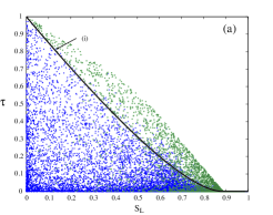
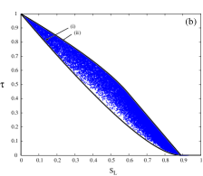
Figure 1: Plot of the tangle, $\tau$, and linear entropy, ${\cal S}_{L}$, of numerically generated two-qubit random matrices. Two sets of data are plotted: a) 30,000 randomly generated matrices, which show the extent of physical states in the entanglement-purity plane; b) 30,000 randomly generated matrices weighted to explore the boundary region. Also shown are analytical curves for: i) the Werner state, a mixture of the maximally-entangled state and the maximally-mixed state; and ii) the maximally-entangled mixed states, states with the maximal amount of entanglement for a given degree of linear entropy (or vice versa). See text for further details.

In Fig. (1a) we have also explicitly plotted the tangle versus linear entropy for the Werner state, a mixture of the maximally-entangled state and the maximally-mixed state Werner89 :

$$\hat{\rho}={{1-\gamma}\over{4}}I_{2}\otimes I_{2}+\gamma|\Phi_{+}\rangle\langle\Phi_{+}|,$$ (4)

where $I_{2}$ is the identity matrix and $|\Phi_{+}\rangle={1\over\sqrt{2}}\left[|0\rangle|0\rangle+|1\rangle|1\rangle\right]$. We have labelled our orthogonal qubit states by $|0\rangle$ and $|1\rangle$. This Werner state is entangled (inseparable) for $\gamma>1/3$Bennett96a and maximally-entangled when $\gamma=1$. The results from Fig. (1a) clearly indicate a class of states that have a larger degree of entanglement for a given linear entropy than the Werner states. We also generated a second set of data (by random perturbations about the maximally-entangled mixed states) so as to examine the boundary of possible states, which in the previous data set was a sparsely populated region. As can be seen in Fig. (1b), a definite boundary to the physically possible states exists.

Let us now analytically determine the form of these maximally-entangled mixed states (MEMS). As our starting point, let us consider the Werner state given by (4). How can one increase its degree of entanglement without changing its purity, or, alternatively, how can one increase its linear entropy given a certain degree of entanglement? In deriving our ansatz we will note the following points:

• In the Werner state (4) all the entanglement arises from the $\gamma|\Phi_{+}\rangle\langle\Phi_{+}|$ term, and hence, to leave the degree of entanglement fixed while increasing the linear entropy this term needs to remain untouched. Local unitary operations will not affect the degree of entanglement or linear entropy.

• The $I_{2}\otimes I_{2}$ term of the Werner states comprises the maximally-mixed state. It can be written as an equal incoherent mixture of the four Bell states

  $$|\Psi_{\pm}\rangle = {1\over\sqrt{2}}\left[|0\rangle|1\rangle\pm|1\rangle|0\rangle\right],$$ (5)

  $$|\Phi_{\pm}\rangle = {1\over\sqrt{2}}\left[|0\rangle|0\rangle\pm|1\rangle|1\rangle\right],$$ (6)

  In our ansatz, if we increase the amount of any of the $|\Psi_{\pm}\rangle$ or $|\Phi_{-}\rangle$ Bell states, then the net entanglement in the total system generally decreases.

• In a general two-qubit density matrix there are two types of off-diagonal terms, those that represent the entanglement and those that represent single particle superposition. These single particle superposition terms can be set to zero by local linear operations, and so, by definition, cannot change the net entanglement.

• The diagonal elements of the two-qubit density matrix do not affect the system’s maximum entanglement (given a specified amount of $|\Phi_{+}\rangle\langle\Phi_{+}|$. The diagonal elements, however, have a significant impact on the linear entropy.

These principles lead us to postulate an ansatz of the form

$$\hat{\rho}=\left(\begin{array}[]{cccc}x+{\gamma\over 2}&0&0&{\gamma\over 2}\\ 0&a&0&0\\ 0&0&b&0\\ {\gamma\over 2}&0&0&y+{\gamma\over 2}\\ \end{array}\right).$$ (11)

This comprises a mixture of the maximally-entangled Bell state $|\Phi_{+}\rangle$ and a mixed diagonal state (who populations are specified by the real and non-negative parameters a,b,x,y). Without loss of generality we choose $\gamma$ to be a positive real number, which ensures that the ansatz density matrix is positive semi-definite. From normalization,

$$x+y+a+b+\gamma=1,$$ (12)

The linear entropy is simply given by

$${\cal S}_{L}={4\over 3}\left\{1-a^{2}-b^{2}-x^{2}-y^{2}-\gamma\left(x+y\right)-\gamma^{2}\right\}$$ (13)

with the concurrence given by

$${\cal C} = {\rm Max}\left[\gamma-2\sqrt{ab},0\right].$$ (14)

To determine the form of the two-qubit maximally-entangled mixed states, we begin by specifying that the concurrence ${\cal C}$ must be greater than zero. Thus ${\cal C}={\rm Max}\left[\gamma-2\sqrt{ab},0\right]=\gamma-2\sqrt{ab}\geq 0$ and therefore is maximized when ${\cal C}=\gamma$. This requires either $a=0$ and/or $b=0$ (without loss of generality we set $b=0$). Using the normalization constraint given by (12), the linear entropy is given by

$${\cal S}_{L}={4\over 3}\left\{2a+\left(\gamma+2x\right)\left(1-a-\gamma\right)-2x^{2}-2a^{2}\right\}.$$ (15)

Calculating the turning point of (15) we find that $\partial{\cal S}_{L}/\partial x=0$ when either $x=0$ (a minimum) or $2x=1-a-\gamma$ (a maximum) and $\partial{\cal S}_{L}/\partial a=0$ when either $a=0$ (a minimum) or $4a=2-2x-\gamma$ (a maximum). First examining the $\partial{\cal S}_{L}/\partial x$ stationary solution and the maximum given by $2x=1-a-\gamma$, we observe that this condition requires $x=y$. If $a=1-\gamma$ then the stationary point corresponds to a turning point. We now need to examine several parameter regimes to determine the optimal solution. The first region has concurrence values in the region $2/3\leq{\cal C}\equiv\gamma\leq 1$. In this region the optimal situation occurs when $x=0$ and $a=1-\gamma$. This means the maximally-entangled mixed state has the form

$$\hat{\rho}_{\rm\scriptsize MEMS}=\left(\begin{array}[]{cccc}{\gamma/2}&0&0&{\gamma/2}\\ 0&1-\gamma&0&0\\ 0&0&0&0\\ {\gamma/2}&0&0&{\gamma/2}\\ \end{array}\right).$$ (20)

The second regime occurs for $0\leq{\cal C}\equiv\gamma\leq 2/3$. In this case the optimal solution occurs when $a=1/3$ and $x+\gamma/2=1/3$. The optimal maximally-entangled mixed state in this region has the form

$$\hat{\rho}_{\rm\scriptsize MEMS}=\left(\begin{array}[]{cccc}{1/3}&0&0&{\gamma/2}\\ 0&{1/3}&0&0\\ 0&0&0&0\\ {\gamma/2}&0&0&{1/3}\\ \end{array}\right).$$ (25)

In this case the diagonal elements do not vary with $\gamma$. Combining both these solutions, we can obtain (up to local unitary transformations) the following single explicit form for the maximal entangled mixed state:

$$\hat{\rho}_{\rm\scriptsize MEMS}=\left(\begin{array}[]{cccc}g(\gamma)&0&0&{\gamma/2}\\ 0&1-2g(\gamma)&0&0\\ 0&0&0&0\\ {\gamma/2}&0&0&g(\gamma)\\ \end{array}\right),$$ (30)

where

$$g(\gamma)=\left\{\begin{array}[]{cccc}\gamma/2&&&{\cal C}\equiv\gamma\geq 2/3\\ 1/3&&&{\cal C}\equiv\gamma<2/3\end{array}\right..$$ (33)

The degree of entanglement for this maximally-entangled mixed state is simply $\tau=\gamma^{2}$, while the linear entropy has the form

$${\cal S}_{L} = \frac{2}{3}\left[4\,g(\gamma)\,\left(2-3\,g(\gamma)\right)-\gamma^{2}\right].$$ (34)

In figure (1) we have plotted the tangle versus the linear entropy for the Werner state, and the numerically determined maximally-entangled mixed state. Our analytic expression for the state (30) perfectly overlays the numerically generated optimal curve. It is clear that these states have a significantly greater degree of entanglement for a given linear entropy than the corresponding Werner states. The maximally-entangled mixed state and Werner state curves join each other at two points in the tangle - linear entropy plane. The first and most obvious point occurs at $(\tau,S_{L})=(1,0)$ (here both states are maximally entangled). The second point occurs at $(\tau,S_{L})=(0,8/9)$. Here the two states are given by,

$$\hat{\rho}_{\rm\scriptsize WERNER}=\left(\begin{array}[]{cccc}{1\over 3}&0&0&{1\over 6}\\ 0&{1\over 6}&0&0\\ 0&0&{1\over 6}&0\\ {1\over 6}&0&0&{1\over 3}\end{array}\right),\;\;\hat{\rho}_{\rm\scriptsize MEMS}=\left(\begin{array}[]{cccc}{1\over 3}&0&0&0\\ 0&{1\over 3}&0&0\\ 0&0&0&0\\ 0&0&0&{1\over 3}\end{array}\right).$$ (43)

Neither state is entangled. We observe that $\hat{\rho}_{\rm\scriptsize MEMS}$ at this point has no nonzero off-diagonal elements but the Werner state does. The maximally-entangled mixed state is entangled as soon as the off-diagonal elements are nonzero ($\gamma>0$, while the Werner state requires $\gamma>1/3$ to be entangled). Though $\hat{\rho}_{\rm\scriptsize WERNER}$ and $\hat{\rho}_{\rm\scriptsize MEMS}$ have different forms they have the same degree of entanglement (zero) and linear entropy. Because of the way the maximally-entangled mixed state has been constructed, it never attains a linear entropy $S_{L}=1$. The Werner state attains this point because of its maximally-mixed component.

To confirm that our analytic solution is optimal and that no density matrix has a greater degree of entanglement for a given linear entropy than the state (30), we generated one million further random density matrices. We found that the maximally-entangled mixed state is indeed optimal. It is interesting to note, however, that the state is only optimal for mixture measures based on ${\rm Tr}\left[\hat{\rho}^{2}\right]$; if instead the degree of mixture is measured for instance by the entropyvonNeumann55 the state is not optimal.

Lastly, how does our class of maximally-entangled mixed states compare with those predicted by Ishizaka and HiroshimaIshizaka00 ? Ishizaka’s two-qubit mixed states, the Werner state being a specific example, were chosen so that the degree of entanglement of such states cannot be increased further by unitary operations. In contrast we have derived a class of states that have the maximum amount of entanglement for a given linear entropy (and vice versa). Therefore our states are members of the Ishizaka et al. class by definition, although they were not explicitly consideredIshizaka00 . The Ishizaka et al. result indicates that a maximally-entangled mixed state cannot have the degree of entanglement increased by unitary operations. This state can however have its entanglement increased by a simple and experimentally realizable non-unitary concentration protocol recently proposed by Thew and MunroThew00 . Such a protocol is a based on generalization of the Procrustean method originally introduced for pure statesBennett96b and recently demonstrated experimentallyKwiat 00 . In Figure (2) we display the results of the concentration protocol for two initial conditions. The solid curves represent a range of states that are obtainable, from the maximally-entangled mixed state, as the concentration protocol is applied to improve the output state characteristics. We observe that for all $\gamma$ the output characteristics can be significantly improved (solid grey lines). In fact for $\gamma\geq 2/3$ the maximally-entangled mixed state can be concentrated up the dashed curve to a maximally-entangled pure state.

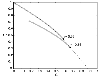
Figure 2: Plot of the tangle $\tau$ versus linear entropy $S_{L}$ for the maximally-entangled mixed state (dotted line). By employing a concentration protocol[26], an initial state (solid circle), can be manipulated to produce a range of new states (solid grey lines) with improved entanglement and linear entropy characteristics.

To summarize, we have discovered a class of partially entangled mixed two-qubit states that have the maximum amount of entanglement for a given linear entropy. An analytical form for these states was derived and they were shown to have significantly more entanglement for a given degree of purity than the Werner states. The properties of these states are still largely unknown and require significant exploration. Open questions such as “can such states be realized experimentally”, “to what extent do they violate Bell inequalities?”, and “do they have information processing advantages over other states” are the subject of current investigation.

We wish to thank K. Nemoto and G. J. Milburn for encouraging discussions. WJM and AGW would like to acknowledge the support of the Australian Research Council while DFVJ would like to thank the University of Queensland for their hospitality during his visit.

References

- (1) D. P. DiVincenzo, Science 270, 255 (1995).
- (2) V. Vedral et al., Prog. Quant. Electron. 22, 1 (1998).
- (3) B. Schumacher, Phys. Rev. A 54, 2614 (1996).
- (4) A. K. Ekert, Phys. Rev. Lett 67, 661 (1991).
- (5) T. Jennewein et al., Phys. Rev. Lett 84, 4729 (2000); D. S. Naik et al., ibid, 4733 (2000); W. Tittel et. al, ibid, 4739 (2000).
- (6) C. H. Bennett et al., Phys. Rev. Lett 70, 1895 (1993).
- (7) D Bouwmeester et al., Nature 370. 575, 1997; D. Boschi et. al, Phys. Rev. Lett 80, 1121 (1998).
- (8) R. Cleve et al., Phys. Rev. Lett 82, 648 (1999).
- (9) A. Aspect et al., Phys. Rev. Lett49, 91 (1982); A. Aspect et al., Phys. Rev. Lett 49, 1804 (1982).
- (10) P. G. Kwiat et al., Phys. Rev. A 60, R773 (1999).
- (11) Q. A. Turchette, et al., Phys. Rev. Lett 81, 3631 (1998); C. A. Sackett et al., Nature 404, 256 (2000).
- (12) Q. A. Turchette et al., Phys. Rev. Lett 75, 4710 (1995).
- (13) S. L. Braunstein, et al., Phys. Rev. Lett 83, 1054 (1999).
- (14) I. L. Chuang et al., Phys. Rev. Lett 80, 3408 (1998).
- (15) A.G. White, D.F.V. James, P.H. Eberhard, and P.G. Kwiat, Phys. Rev. Lett 83, 3103 (1999).
- (16) A.G. White, D.F.V. James, W.J.Munro and P.G. Kwiat, submitted to Science (2001).
- (17) Arbitrary two-qubit states are uniquely specified by 15 real parameters [8]. The degree of entanglement and mixture do not determine all these 15 parameters absolutely.
- (18) C. H. Bennett, et al., Phys. Rev. A 54, 3824 (1996).
- (19) S. Ishizaka and T. Hiroshima, quant-ph/0003023.
- (20) R. F. Werner, Phys. Rev. A 40, 4277 (1989).
- (21) V. Coffman et al., Phys. Rev. A 61, 052306 (2000); quant- ph/ 9907047
- (22) J. von Neumann, Mathematical Foundations of Quantum Mechanics. (Princeton University Press, Princeton, 1955) (Eng. translation by R. T. Beyer).
- (23) S. Bose et al., Phys. Rev. A61 040101(R) (2000).
- (24) K Zyczkowski, Phys. Rev. A58, 883 (1998); Phys. Rev. A60, 3496 (1999)
- (25) C. H. Bennett, et al., Phys. Rev. Lett 76, 722 (1996).
- (26) R. T. Thew and W. J. Munro, in press Phys. Rev. A (2001)
- (27) C.H. Bennett, et al., Phys. Rev. A 53, 2046 (1996).
- (28) P. G. Kwiat et. al, Nature 409, 1014 (2001) (2001)