Indian Journal of Theoretical Physics 48, no. 2, pp. 97-132 (2000)

On the nature of spin, inertia and gravity
of a moving canonical particle

Volodymyr Krasnoholovets

Institute of Physics, National Academy of Sciences,

Prospect Nauky 46, UA-03028 Kyïv, Ukraine   http://inerton.cjb.net

October 1998 – November 1999

Abstract

It is suggested that a moving canonical particle interacts with a vacuum regarded as a ”soft” cellular space. The interaction results into the emergence of elementary excitations of space – inertons – surrounding the particle. It is assumed that such a motion leads not only to the spatial oscillation of the particle along a path but to the oscillation of the particle centre-of-mass as well. This phenomenon culminating in the anisotropic pulsation of the particle is associated with the notion of spin. The particle-space interaction is treated as the origin of the matter waves which are identified with the particle inertia and inertons surrounding the moving particle are considered as carriers of its inert properties. Inertons are also identified with real carriers of the gravitational interaction and the range of the particle gravitational potential is evaluated by the inerton cloud amplitude $\Lambda=\lambda c/v_{0}$, where $\lambda$ is the de Broglie wavelength, $c$ and $v_{0}$ are the velocity of light and the particle respectively. The nature of the phase transition that occurs in a quantum system when one should pass from the description based on the Schrödinger formalism to that of resting on the Dirac one is explained in detail.

Key words:

quantum mechanics, spin, space, inertons, gravitation

PACS:

03.65.w Quantum mechanics;
04.50 Unified field theories and other theories of gravitation;
04.60.-m Quantum gravity

1 Introduction and the statement of problem

Since the introduction of a hypothesis for the spin by Goudsmit [1] and Uhlenbeck [2] (see also Van der Waerden [3]), the question as to the nature of this phenomenon has consistently been a major focus of interest for researchers. Most of them are guided by the findings of Schrödinger [4] and subsequently of Dirac [5] who have shown that a rapid oscillatory motion – Zitterbewegung – is peculiar to a free relativistic particle. Then Frenkel [6] has assumed that the spin can be regarded as a proper mechanical moment, which is due to the fuzzy mass and charge hidden from an observer. The ideas of Schrödinger and Frenkel have stimulated the emergence of such particle spin models as bilocal rotator, Halbwachs et al. [7], relativistic oscillator, Ginzburg and Man’ko [8], and stochastic oscillator, Petroni et al. [9], dequantized spin-particle, Plahte [10], and extended objects, Umezawa [11], Barut and Tracker [12], Bohm et al. [13]. Barut and Zanghi [14] have considered the spin as an angular moment of the real Zitterbewegung. Spavieri [15] has described the spin of the particle by the intrinsic component, a massless subparticle that travels around the centre-of-mass of the particle in a fuzzy orbit. Berezin and Marinov [16] and Srivastava and Lemos [17] have treated the spin as a construction of hidden variables that obey Grassmann’s algebra. Kuryshkin and Entralgo [18] have discussed the classical spin model based on the concept of a structural-point object that implies an assembly of point particles with distinctive small masses and charges confined to a specific interaction, which operates between them. On the other hand, Ohanian [19] includes the assumption that neither the spin, nor the magnetic moment of the electron are its intrinsic properties and that they are nothing but the structure of the field of the electronic wave. By assuming that the intrinsic magnetic moment of the electron is the initial notion, Heslot [20] associates the emergence of the spin with the generator of a group of rotations in nonrelativistic classical mechanics. Presented by Shima [21] is the field Lagrangian that satisfies the gauge invariance and describes the spin-1/2 massless Dirac particle. Pav$\rm\check{s}$i$\rm\check{c}$ et al. [22] have developed the model proposed by Barut and Zanghi [14] in terms of Clifford algebra; Pav$\rm\check{s}$i$\rm\check{c}$ et al. have obtained a non-linear Dirac-like equation which characterises a cylindrical helix trajectory of a point-like object, i.e. spinning particle. Corben [23] has proposed an interesting approach to the structure of a spinning point particle at rest. Sidharth [24] has conjectured that spin is a consequence of a space-time cut off at the Compton wavelength and Compton time scale. Oudet [25] has maintained the deep analysis of experimental manifestations of the spin and the model of the electron in which the electron is thought as a small fluid mass has been discussed. The shape of the mass is supposed to be transformed according to the energy exchanged between the field and the electron along its trajectory. This conception proposes that there is energy associated with the spin. It is notable that the author’s following study is roughly similar to the pattern described by Oudet.

In the above papers, a variety of notions, in some instances mutually exclusive ones, provide the basis for the development of the spin model, and yet some specificity that must necessarily be inherent in an elementary particle is the initial point. The present paper also deals with the spin problem. However the author pursues an object to study the problem in the framework of a vacuum medium model. And in this case the so-called hidden variables (see, e.g. Bohm [26]) evidently should play a primordial important role.

There are several new views on the vacuum substance (see, e.g. Fomin [27], Aspden [28], and Vegt [29]). On special note is approaches developed by Winterberg [30] and Rothwarf [31]. Winterberg’s aether is a densely filled substance with an equal number of positive and negative Planck masses $m_{\rm P}=\sqrt{hc/G}$ which interact locally through contact-type delta-function potentials; in the framework of this approach Winterberg has shown that quantum mechanics can be derived as an approximate solution of the Boltzmann equation for the Planck aether masses. The particle in that model is a formation appeared owing to the interaction between the positive and negative Planck masses similar to the phonon in a solid.

The Rothwarf’s aether model [31] is based upon a degenerate Fermion fluid, composed primarily of electrons and positrons in a negative energy state relative to the null state or true vacuum. A key assumption of Rothwart was that the speed of light was the Fermi velocity of the degenerate electron-positron plasma that dominates the aether. The model was applied for the description of a large number of phenomena such as the nature of spin (considered as a vortex in the aether), electric fields (polarization of the aether), the nature of the photon (a region of rotating polarized aether propagating with a screw-like motion), etc.

The author’s vacuum concept [32-34] is close to that of Winterberg [30]. However, unlike Winterberg’s aether, it supposes an elasticity of discrete vacuum substance and takes into account the possibility of deterministic motion of a particle in real space. It is the first physical model of space that is not contradictory to the formalism of special relativity (see Ref. [33]). At the same time the concept conjectures a new type of elementary excitations of space – inertons, – which should substitute for gravitons of general relativity. The statement needs an explanation. As we know classical mechanics was the origin both of the theory of relativity and quantum mechanics. In classical mechanics an object’s mass can manifest itself as gravitational mass (in gravitational experiments) or as inert one (in the dynamics including the kinetics). General relativity asserts (see, e.g. Bergmann [35]) that gravitational and inert mass are equivalent. However, the affirmation was proved in the case of macroscopic phenomena: The theory of relativity derives the equations of motion of a massive point in the highly rarefied space (see, e.g. Bergmann [36], Pauli [37], Weinberg [38], Dubrovin et al. [39]). Recent developments in quantum general relativity (see, e.g. Ashtekar [40]) do not concern this significant problem as well.

Quantum mechanics does not tell one notion of mass from the other one and in addition the equations of quantum mechanics include mass only as a pure classical parameter. So orthodox quantum theory can say nothing about the mass behaviour in atom and nucleus range. Sidharth [41] tried to study this problem; he concluded that inert mass of an elementary particle is the energy of binding of nonlocal amplitudes in the zitterbewegung Compton wavelength region. But what energy is?! When applied to a particle, the energy means the square form: the mass times the velocity to the second power. Much probably in this case just the notion of mass is initial. What is more, the submicroscopic construction of quantum mechanics developed at the scale of $10^{-28}$ cm in the author’s research [32-34] evidences that the notion of inert mass is original. The moving particle interacts with space which is not empty but fine-grained, in any event ”so-called empty space is actually filled with elementary particles that pop in and pop out and … these ”virtual” particles … could exert a gravitational force”, Krauss [42]). As a consequence, elementary deformation excitations caused by that interaction must accompany the moving massive point. This means that the Einstein classical equations which describe the mass distribution in empty space should not only be added by the lambda term but they are bound to be change: The equations should be constructed with due regard for the interaction of the moving mass/masses with space as well. When such is the case, the mentioned excitations, i.e. inertons, will play a role of actual carriers of gravitational interaction. It must be emphasized that clouds of inertons surrounding electrons, indeed, manifest themselves experimentally; the statement has recently been proved by the author[43].

The author has previously demonstrated [32,33] that the mechanics of a massive point, which was interacting with space, culminated in the Schrödinger wave equation formalism. In the present paper the investigation of the behaviour of a massive particle with the spin is performed and it is shown how such kind of the submicroscopic mechanics can give rise to the Dirac equation formalism. Besides the proposed paper gives a coherent explanation, as compared to author’s preceding papers on the inerton motion, notions of space, and the space crystallite and peculiar features of the latter are discussed.

2 Intrinsic motion of a particle

Space is treated by the author [32-35] as a specific medium (a quantum aether) with a cellular structure, each cell being either the superparticle or corpuscle filled (i.e. this is a mathematical space constructed of balls). The corpuscle is thought to evolve from the superparticle when degeneration over one of its multiplet states is eliminated. The velocity of light $c$, i.e. the speed of the transmission of information from superparticle to superparticle, is a property of space. Superparticles do not transfer in space and yet they are capable of conveying information by a relay mechanism. As for the corpuscle, it actually travels passing between fluctuating superparticles. We will identify the corpuscle with a canonical particle like the electron, muon, and so on.

In the present model, the initial velocity $v_{0}$ of the particle is not constant along its trajectory due to permanent mutual collisions with superparticles. If the particle is not absolutely rigid it can be presumed that along with a nonstationary translational movement, the particle also exhibits a nonstationary intrinsic motion, i.e. owing to mutual collisions with space, radial pulsation is excited in the particle (a relative motion of the front and back surfaces along the line coincident with the particle trajectory).

In paper [33] the Lagrangian of a relativistic spinless particle has been chosen in the form:

$$L=-M_{0}c^{2}\Bigl{\{}1-\bigl{[}\dot{X}^{2}+\sum_{r}U(X,\dot{X};x_{(r)},\dot{x}_{(}r))\bigr{]}/c^{2}\Bigr{\}}^{1/2}$$ (1)

where $M_{0}$ is the mass of the particle at rest. The function $U$ allows for the kinetic energy of the particle-emitted inerton ensemble and the potential of the interaction between the particle and inertons. In (1) the translational motion of the physical ”point” (particle cell) along its trajectory is described by the radius vector $X(X^{i})$ and the velocity vector $\dot{X}({\dot{X}}^{i})$; similarly, $x_{(r)}(x_{(r)}^{i})$ and ${\dot{x}}_{(r)}({\dot{x}}_{(r)}^{i})$ are the radius vector and velocity vector of the $r$th inerton. Let us modernise the Lagrangian (1) by introducing the function $U_{1}$, which incorporates the intrinsic motion of the particle and inerton ensemble

$$L=-M_{0}c^{2}\Bigl{\{}1 - \bigl{[}\dot{X}^{2}+\sum_{r}U(X,\dot{X};x_{(r)},\dot{x}_{(r)})$$ (2)

$$+ \sum_{r}U_{1}(\Xi,\dot{\Xi};\xi_{(r)},\dot{\xi}_{(r)})\bigr{]}/c^{2}\Bigr{\}}^{1/2}.$$

We suppose that the intrinsic motion of the particle is related with the oscillation of the particle’s centre-of-mass and is a consequence of an asymmetric deformation of the particle volume at the initial moment at which the particle acquires a momentum. Indeed, as the particle is considered to be solid and elastic (like a drop), then the induction of the convace on one side must automatically result in the appearance of the convex on the other side (Fig. 1). However the elasticity also implies the appearance of the reverse force which restores the particle state. We will examine the intrinsic motion of the particle in the same frame of reference that the spatial motion. Because of this, one will describe the deflected position of the particle centre-of-mass along the particle trajectory by the radius-vector $\Xi(\Xi^{i})$ and depict the speed of its motion by the intrinsic-velocity vector $\dot{\Xi}({\dot{\Xi}}^{i})$; in a similar way, $\xi_{(r)}$ and ${\dot{\xi}}_{(r)}$ are the radius-vector and velocity of the intrinsic motion of the rth inerton. It should be noted that the point over the vectors $\dot{X}$ and $\dot{\Xi}$ means differentiation with respect to the proper time t of the particle which characterises the particle along its trajectory; by analogy, the point over the vectors ${\dot{x}}_{(r)}$ and ${\dot{\xi}}_{(r)}$ implies differentiation on the proper time $t_{(r)}$ of the $r$th inerton.

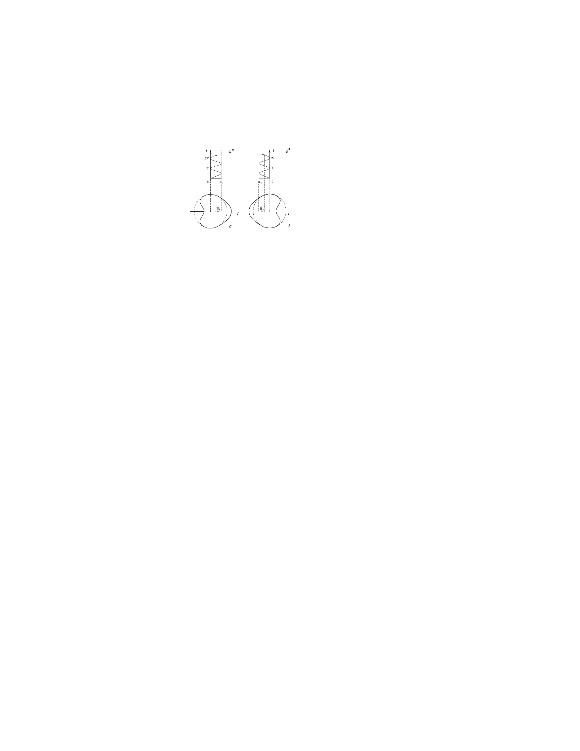
Figure 1: The pulsation of the particle along its spatial trajectory: $a$ the convex is oriented in the direction of the particle spatial motion and this orientation determines the intrinsic-velocity vector $\dot{\Xi}_{\uparrow}$; $b$ the convex is oriented against the particle spatial motion and this orientation determines the intrinsic-velocity vector $\dot{\Xi}_{\downarrow}$. Figures $a^{*}$ and $b^{*}$ schematically show the trajectory of the particle centre-of-mass in a frame of reference connected with the cell, which includes the oscillating particle ($\alpha_{0}$ is the amplitude of these intrinsic oscillations).

In the intrinsic motion one of the two possibilities can be realized: either the position of the particle’s centre-of-mass is displaced forward from the equilibrium one (Fig. 1$a$) or, on the contrary, the position of the particle’s centre-of-mass is displaced backwards from the one (Fig. 1$b$). Then, in the former case, the intrinsic velocity vector $\dot{\Xi}$ is aligned with the translational motion of the particle, i.e. parallel to the vector $\dot{X}$; in the latter case, it is opposing the translational motion, i.e. antiparallel to the vector $\dot{X}$. The same is also true for the vector of the intrinsic velocity of inertons. In order to discern these two phase states of radial pulsations of the particle, let us use the index $\alpha$ for the intrinsic-velocity vector of the particle and of the $r$th inerton that defines the intrinsic-velocity projection on the respective trajectories of the particle and the $r$th inerton. One presumes that $\alpha=\uparrow$ for the former case (the motion-oriented projection) and $\alpha=\downarrow$ for the latter case (the motion-opposing projection). Thus, hereinafter, we shall use the notations ${\dot{\Xi}}_{\alpha}$ and ${\dot{\xi}}_{\alpha}$ for the intrinsic-velocity vectors.

Allowances can be made for the two possible phase states of the particle in the Lagrangian if it is given as the two-row matrix

$${\cal L}={{\cal L}_{\uparrow}\choose{\cal L}_{\downarrow}}.$$ (3)

Let us represent the function ${\cal L}_{\alpha}$ in the form (compare with Ref. [32]):

$${\cal L}_{\alpha}=-gc^{2}\bigl{\{}1-[U^{\rm spat}+U^{\rm intr}_{\alpha}]/gc^{2}\bigr{\}}^{1/2},$$ (4)

$$U^{\rm spat}=g_{ij}\dot{X}^{i}(t)\dot{X}^{j}(t)+\sum_{r}\tilde{g}_{ij}^{(r)}\dot{x}^{i}_{(r)}(t_{(r)})\dot{x}^{j}_{(r)}(t_{(r)})\ \$$

$$-\sum_{r}\frac{2\pi}{T_{(r)}}\delta_{t-\Delta t_{(r)},t_{(r)}}\Bigl{[}X^{i}(t)\hat{B}_{ij}\dot{x}^{j}_{(r)}(t_{(r)})+\dot{X}^{i}(t)\big{|}_{t=0}\hat{B}_{ij}x^{j}_{(r)}(t_{(r)})\Bigr{]};$$ (5)

$$U^{\rm intr}=g_{ij}{\dot{\Xi}}_{\alpha}^{i}(t){\dot{\Xi}}_{\alpha}^{j}(t)+\sum_{r}\tilde{g}_{ij}^{(r)}{\dot{\xi}}^{i}_{\alpha(r)}(t_{(r)}){\dot{\xi}}^{j}_{\alpha(r)}(t_{(r)})$$

$$\ \ \ \ \ \ \ \ \ -\sum_{r}\frac{2\pi}{T_{(r)}}\delta_{t-\Delta t_{(r)},t_{(r)}}\Bigl{[}\Xi^{i}_{\alpha}(t)\hat{B}_{ij}\dot{\xi}^{j}_{\alpha(r)}(t_{(r)})+{\dot{\Xi}}^{i}_{\alpha}(t)\big{|}_{t=0}\hat{B}_{ij}\xi^{j}_{\alpha(r)}(t_{(r)})\Bigr{]};$$ (6)

In (5) the three terms describe the kinetic energies of the particle and of the inerton ensemble and their interaction energy respectively. In (6) the three terms describe the kinetic energies of the intrinsic motion of the particle and of the inerton ensemble and the energy of the intrinsic interaction between the particle and the inerton ensemble accordingly. In (5) and (6) $g_{ij}$ are components of the metric nonparametrised tensor created by the particle in the three-dimensional space, along the particle trajectory  $g_{ij}={\rm const}\ {\delta}_{ij}$;   $g=g_{ij}\delta^{ij}$ is the convolution of the tensor. The $r$th inerton moves in the field $g_{ij}$ and is characterized by the proper metric tensor with the components ${\tilde{g}}^{(r)}_{ij}$ in the three-dimensional space; these components describe a local deformation of space in the neighborhood of the $r$th inerton (the index $r$ is enclosed in parentheses in order to distinguish it from the indices $i,\ j$, and $s$ which represent the vector and tensor quantities). Along the trajectory of the $r$th inerton, the tensor ${\tilde{g}}^{(r)}_{ij}$ is locally equal to   const$\ {\delta}_{ij}$  approximately.  $1/{T_{(r)}}$ is the frequency of mutual collisions between the particle and the $r$th inerton, hence, $T_{(r)}$ is the time interval elapsed from the moment of emission of the $r$th inerton to the moment of its absorption; ${\delta}_{t-{\Delta t_{(r)}},t_{(r)}}$ is the Kroneker’s symbol that provides an agreement between the proper time $t$ of the particle and the proper time $t_{(r)}$ of the $r$th inerton and $\Delta t_{(r)}$ is the time interval after the elapse of which (starting from the moment of the particle motion $t=0$) the particle emits the $r$th inerton. Besides in (5) and (6) the notation

$$\hat{B}_{ij}=\sqrt{g_{is}(\hat{A}^{-1}\tilde{g}_{sj}^{(r)})_{0}},$$ (7)

is introduced where the operator ${\hat{A}}^{-1}$ takes inertons to the trajectories distinct from the trajectory of the particle [32].

Below we shall employ the approximation where the quantities ${\hat{B}}_{ij}$ are constant; for this purpose the proper time $t$ of the particle should be regarded as the parameter proportional to the natural $l$,   $t\propto l$  ($l$ is the trajectory length). In this case, the Euler-Lagrange equations for the variables ($X^{i},{\dot{X}}^{i}$) and ($x_{(r)},{\dot{x}}_{(r)}$) agree with the respective equations of extremals for the nonrelativistic Lagrangian [32,33]. Similarly obtainable are the equations for the intrinsic variables  (${\Xi}^{i}_{\alpha},{\dot{\Xi}}^{i}_{\alpha}$)  and  (${\xi}^{i}_{\alpha,(r)},{\dot{\xi}}^{i}_{\alpha,(r)}$).  As the proper time $t$ of the particle is related with that of the $r$th inerton by means of the relation $t=t_{(r)}+{\Delta}t_{(r)}$, the equations of extremals for the intrinsic variables can be written through the parameter $t_{(r)}$.

In the Euclidean space the Euler-Lagrange equations for the intrinsic variables of the Lagrangian (4) take the form (compare the respective equations for space variables in Refs. [32, 33])

$$\ddot{\Xi}_{\alpha r}(t_{r})+\frac{\pi}{T_{r}}\frac{v_{0r}}{c}\dot{\xi}_{\alpha r}^{\perp}(t_{r})=0;$$ (8)

$$\ddot{\xi}^{\perp}_{\alpha r}(t_{r})-\frac{\pi}{T_{r}}\frac{c}{v_{0r}}\Bigl{[}\dot{\Xi}_{\alpha r}(t_{r})-\dot{\Xi}_{\alpha r}(t_{r})\big{|}_{t_{r}=0}\Bigr{]}=0;$$ (9)

$$\ddot{\xi}^{\parallel}_{\alpha r}(t_{r})=0,$$ (10)

from this point on, the index $r$ is not parenthesis. In Eqs. (8) and (9) the intrinsic vectors ${\ddot{\Xi}}_{{\alpha}r}$ and ${\dot{\Xi}}_{{\alpha}r}$ are oriented parallel or antiparallel to the $X\equiv X^{1}$ axis, along which the particle moves; ${\dot{\xi}}^{\perp}_{{\alpha r}}=\sqrt{({\dot{\xi}}^{2}_{{\alpha}r})^{2}+({\dot{\xi}}^{3}_{{\alpha}r})^{2}}$ is the intrinsic-velocity vector projection of the $r$th inerton that is oriented parallel or antiparallel to the axis which is normal to the $X$ axis. In this case, the projection of the intrinsic velocity of inertons onto the $X$ axis is ${\dot{\xi}}^{\parallel}_{{\alpha}r}(t_{r})=0$.

For the sake of convenience, let us represent the intrinsic-velocity vector for the particle and the $r$th inerton in the form (hereinafter, we omit the index $\perp$ at $\xi$)

$$\dot{\Xi}_{\alpha r}(t_{r})=e_{\alpha}\dot{\Xi}_{r}(t_{r}),\ \ \ \ \dot{\xi}_{\alpha r}(t_{r})=e_{\alpha}\dot{\xi}_{r}(t_{r}),$$ (11)

where the polarization symbol is inserted

$$e_{\alpha}=\cases{1&if $\alpha=\uparrow$,\cr-1&if $\alpha=\downarrow$.\cr}$$ (12)

As may be inferred from the form of Eqs. (8) and (9), their solution essentially depends on the quantity of the initial intrinsic velocity of the particle ${\dot{\Xi}}_{\alpha r}(t_{r}){|}_{t_{r}=0}$.  It seems reasonable to relate this value to the quantity of the initial velocity of the particle’s translational motion $v_{o}$ that is typical for the particle on the trajectory; we consider the velocity of light $c$ as peculiar to inertons. Then the initial velocity ${\dot{\Xi}}_{r}\big{|}_{t_{r}=0}$ is determined as

$$\dot{\Xi}_{r}(t_{r})\big{|}_{t_{r}=0}=v_{0r},$$ (13)

where $v_{0r}$ is the velocity of the particle at the moment of its collision with the $r$th inerton [32]:

$$v_{0r}=v_{0}[1-\sin(\pi r/2N)];$$ (14)

$N$ is the total number of the particle-emitted inertons (for $t_{r}\big{|}_{r=0}=t=0$ the quantity $v_{0r}\rightarrow v_{0}$). With regard for the above-mentioned, the solutions for Eqs. (8) and (9) are easily obtainable:

$$\dot{\Xi}_{\alpha r}=e_{\alpha}v_{0r}[1-\sin(\pi t_{r}/T_{r})];$$

$$\Xi_{\alpha r}=e_{\alpha}\Bigl{[}v_{0r}t_{r}+\frac{v_{0r}T_{r}}{\pi}[\cos(\pi t_{r}/T_{r})-1]\Bigr{]};$$

$$\dot{\xi}_{\alpha r}=e_{\alpha}c\cos(\pi t_{r}/T_{r});$$

$$\xi_{\alpha r}=e_{\alpha}{\Lambda_{r}\over\pi}\sin(\pi t_{r}/T_{r}).$$

Solutions (15) and (16) for the intrinsic variables are true only within the time interval $T_{r}=T(1-r/N)$ and they are identical in form to the solutions [33] for space variables $X,\dot{X}$  and   $x^{\perp}_{r},{\dot{x}}^{\perp}_{r}$ (schematically the motion of the particle surrounded by its own inertons is shown in Fig. 2). In (15) and (16) it is put

$$\lambda_{r}=v_{0r}T_{r},\ \ \ \ \ \ \Lambda_{r}=cT_{r}.$$

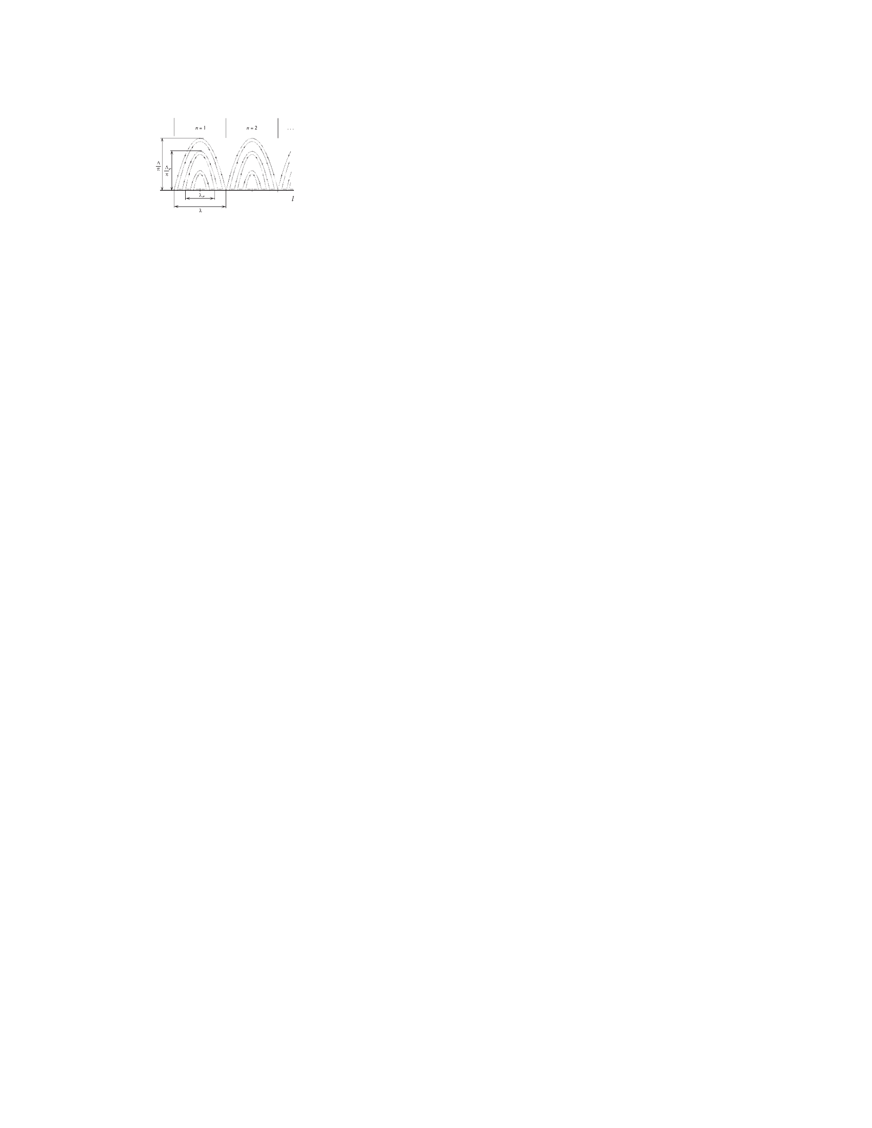
Figure 2: The schematic representation of the motion of the particle surrounded by inertons along the particle trajectory $l$.

Having regard to

$$\dot{X}|_{t=nT}=v_{0}$$

where $n=1,\ 2,\ 3,\ ...$   is the number of the time period $T$ of collisions in accordance with which the quantity of the particle velocity resumes its initial value, one can present [33] the solutions for $X$ and $\dot{X}$ as a function of the proper time $t$ of the particle :

$$\dot{X}(t)=v_{0}(1-|\sin(\pi t/T)|);$$

$$X(t)=v_{0}t+\frac{v_{0}T}{\pi}\Bigl{\{}(-1)^{[t/T]}\cos(\pi t/T)-\bigl{(}1+2[t/T]\bigr{)}\Bigr{\}};$$

here the notation $[t/T]$ means an integral part of the integer $t/T$. By analogy we can write the solutions for the intrinsic variables of the particle that are also true along its entire spatial trajectory (Fig. 3):

$$\dot{\Xi}_{\alpha}(t)=e_{\alpha}v_{0}(1-|\sin(\pi t/T)|);$$

$$\Xi_{\alpha}(t)=e_{\alpha}\Bigl{\{}v_{0}t+\frac{v_{0}T}{\pi}\bigl{\{}(-1)^{[t/T]}\cos(\pi t/T)-\bigl{(}1+2[t/T]\bigr{)}\bigr{\}}\Bigr{\}}$$

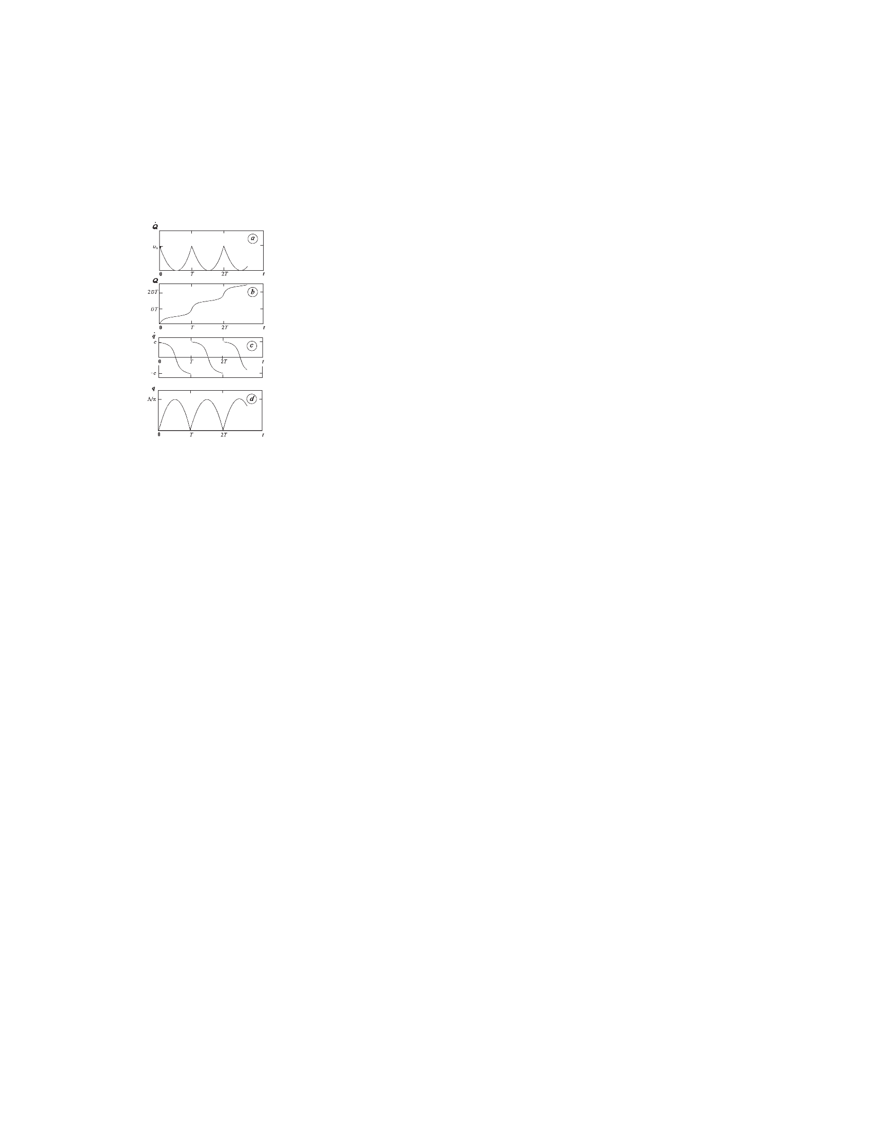
Figure 3: The schematic representation of the solutions of Eqs. (19) and (20) for the particle ($a,\ b$) and Eqs. (23) for the inerton cloud ($c,\ d$). Here $Q\equiv\{X;\ \Xi_{\alpha}\}$, $\dot{Q}\equiv\{\dot{X};\ {\dot{\Xi}}_{\alpha}\}$ and $q\equiv\{x;\ \xi_{\alpha}\}$, $\dot{q}\equiv\{\dot{x};\ {\dot{\xi}}_{\alpha}\}$. Note that the value $\bar{v}T$ shown in the figure b can be interpreted as a mean de Broglie wavelength $<\lambda>$ of the particle along its trajectory.

3 Hamiltonian of a ”bare” particle

Further analysis is performed within the framework of the Euclidean space viewing the inerton ensemble as a single object, i.e. the inerton cloud. Let masses of the particle and the cloud at rest be equal to $M_{0}$ and $m_{0}$ respectively. Assume that the particle trajectory runs along the $X$ axis and let $x$ is the distance between the cloud and the particle, then $\dot{x}$  is the velocity of the cloud in a frame of reference connected with the particle. The intrinsic coordinate $\Xi_{\alpha}=e_{\alpha}\Xi$ defines the location of the centre-of-mass of the pulsating particle along the particle’s trajectory;  the intrinsic-velocity vector ${\dot{\Xi}}_{\alpha}=e_{\alpha}{\dot{\Xi}}$ of the particle sticks out of the point of the particle’s centre-of-mass location. Similarly for the inerton cloud: $\xi_{\alpha}=e_{\alpha}\xi$, where $\xi$ is the displacement of the cloud’s pulsating centre-of-mass from the equilibrium position and $\dot{\xi}_{\alpha}=e_{\alpha}\dot{\xi}$, where $\dot{\xi}$ is the intrinsic-velocity vector that sticks out of the position of the cloud’s centre-of-mass, i.e. $\dot{\xi}$ is the velocity vector of the pulsation. Both the particle’s ($X,{\dot{X}};\Xi,\dot{\Xi}$) and cloud’s ($x,\dot{x};\xi,\dot{\xi}$) parameters are functions of the proper time $t$ of the particle. Thus instead of (3) – (6), we proceed from the Lagrangian $L=\|L_{\alpha}\|$ where

$$L_{\alpha}=-M_{0}c^{2}\Bigl{\{}1\ \ \ \ \ \ \ \ \ \ \ \ \ \ \ \ \ \ \ \ \ \ \ \ \ \ \ \ \ \ \ \ \ \ \ \ \ \ \ \ \ \ \ \ \ \ \ \ \ \ \ \ \ \ \ \ \ \ \ \ \ \ \ \ \ \ \ \ \ \$$

$$-\frac{1}{M_{0}c^{2}}\Bigl{[}M_{0}\dot{X}^{2}+m_{0}\dot{x}^{2}-\frac{2\pi}{T}\sqrt{m_{0}M_{0}}(X\dot{x}+v_{0}x)\Bigr{]}\ \ \ \ \ \ \ \ \ \$$

$$-\frac{1}{M_{0}c^{2}}\Bigl{[}M_{0}\dot{\Xi}_{\alpha}^{2}+m_{0}{\dot{\xi}}_{\alpha}^{2}-\frac{2\pi}{T}\sqrt{m_{0}M_{0}}(\Xi_{\alpha}\dot{\xi}_{\alpha}+e_{\alpha}v_{0}\xi_{\alpha})\Bigr{]}\Bigr{\}}^{1/2}.$$

Here $1/T$ is the frequency of collisions between the particle and the inerton cloud, $v_{0}$ is the initial particle velocity.

If the parameter of running for the functional of extremals

$$S_{\alpha}=\int_{A}^{B}L_{\alpha}dt$$

is thought of as being natural,   $t\propto l$ ($l$ is the $AB$ curve length or in other words the particle path), solution to the Euler-Lagrange equations for both spatial and intrinsic variables of the Lagrangian (21) are readily obtainable. The particle-describing solutions for the variables   ${\dot{X}},X$  and   ${\dot{\Xi}}_{\alpha},\Xi_{\alpha}$  agree with the respective expressions (19) and (20). For solutions for the spatial variables $\dot{x}$ and $x$ of the inerton cloud see Ref. [33] and the solutions for the intrinsic variables of the cloud coincide in form with (16) where the sine and cosine should be put into the modules sign and the index $r$ should be dropped. In other words, the solutions for the cloud have the form

$$q=\frac{\Lambda}{\pi}|\sin(\pi t/T)|;$$

$$\dot{q}=(-1)^{[t/T]}c\cos(\pi t/T)$$

where $q\equiv\{x;\ \xi_{\alpha}\}$ and $\dot{q}\equiv\{\dot{x};\ {\dot{\xi}}_{\alpha}\}$. Note that one can choose the proper time of the particle along its trajectory in the form of $t=l/\bar{v}$ where $\bar{v}$ is the mean velocity of the particle along its trajectory. Owing to expression (19$a$) one finds

$$\bar{v}=\frac{1}{T}\int\limits^{T}_{0}\dot{X}dt=v_{0}(1-2/\pi).$$

With regard for expression (24) the solution of equations of motion for the particle ((19) and (20)) take the symmetric form.

The substitutions

$${\dot{\tilde{x}}}={\dot{x}}-\frac{\pi}{T}\sqrt{M_{0}/m_{0}}\ X,$$

$${\dot{\tilde{\xi}}}_{\alpha}={\dot{\xi}}_{\alpha}-\frac{\pi}{T}\sqrt{M_{0}/m_{0}}\ \Xi_{\alpha}$$

reduce the Lagrangian (21) to the form

$$L_{\alpha}=-M_{0}c^{2}\Bigl{\{}1\ \ \ \ \ \ \ \ \ \ \ \ \ \ \ \ \ \ \ \ \ \ \ \ \ \ \ \ \ \ \ \ \ \ \ \ \ \ \ \ \ \ \ \ \ \ \ \ \ \ \ \ \ \ \ \ \ \ \ \ \ \ \ \ \ \ \ \ \ \ \ \ \ \ \ \ \ \$$

$$-\frac{1}{M_{0}c^{2}}\Bigl{[}M_{0}\dot{X}^{2}-M_{0}\omega^{2}X^{2}+m_{0}\dot{\tilde{x}}^{\ 2}-2\omega\sqrt{m_{0}M_{0}}\ v_{0}x\Bigr{]}\ \ \ \ \ \ \ \ \ \$$

$$-\frac{1}{M_{0}c^{2}}\Bigl{[}M_{0}\dot{\Xi}^{2}_{\alpha}-M_{0}\omega^{2}\Xi^{2}_{\alpha}+m_{0}\dot{\tilde{\xi}}^{\ 2}-2\omega\sqrt{m_{0}M_{0}}\ v_{0}e_{\alpha}\xi_{\alpha}\Bigr{]}\Bigr{\}}^{1/2}$$

where the notation

$$\omega={2\pi}/2T$$

is inserted.

Let us build up the Hamiltonian function appropriate to the Lagrangian (27):

$$H_{\alpha}={\dot{X}}\partial L_{\alpha}/\partial\dot{X}+\dot{\tilde{x}}\partial L_{\alpha}/\partial\dot{\tilde{x}}+\dot{\Xi}_{\alpha}\partial L_{\alpha}/\partial\dot{\Xi}_{\alpha}+\dot{\tilde{\xi}}_{\alpha}\partial L_{\alpha}/\partial\dot{\tilde{\xi}}_{\alpha}-L_{\alpha}.$$

Substituting $L_{\alpha}$ from (27) into (28), we derive

$$H_{\alpha}=M\omega^{2}X^{2}+M\omega^{2}\Xi^{2}_{\alpha}+2\omega\sqrt{mM_{0}}\ v_{0}(x+e_{\alpha}\xi_{\alpha})+Mc^{2}$$

where the designations

$$M=M_{0}/\sqrt{1-v_{0}^{2}/c^{2}},\ \ \ \ \ \ m=m_{0}/\sqrt{1-v^{2}_{0}/c^{2}}$$

are entered (the derivation of (30) presupposes that in the Lagrangians (21) and (27), the radical  $\sqrt{...}$  is constant along the particle trajectory and equal to $\sqrt{1-v_{0}^{2}/c^{2}}$).

On the other hand, the momentum is determined as equal to ${\partial L}/{\partial{\dot{Q}}}$ where $\dot{Q}$ is the canonical velocity. The Lagrangian (27) is a function of the four velocities, so we can introduce their four respective momenta:

$$p=\partial L_{\alpha}/\partial\dot{X}=M\dot{X};$$

$$\tilde{p}\ =\partial L_{\alpha}/\partial\dot{\tilde{x}}\ \ =m\dot{\tilde{x}};$$

$$\pi_{\alpha}=\partial L_{\alpha}/\partial\dot{\Xi}_{\alpha}=M\dot{\Xi}_{\alpha};$$

$$\tilde{\pi}_{\alpha}=\ \partial L_{\alpha}/\partial\dot{\tilde{\xi}}_{\alpha}=m\dot{\tilde{\xi}}_{\alpha}.$$

Expressions (32) permit the Hamiltonian (29) to be represented as

$$H_{\alpha}=p^{2}/M+{\tilde{p}}^{\ 2}/m+\pi^{2}_{\alpha}/M+{\tilde{\pi}}^{\ 2}_{\alpha}/m+(M_{0}c)^{2}/M.$$

Both the Hamiltonians, (30) and (33), are identical and their superposition makes it possible to write the Hamiltonian for the particle – inerton cloud system as

$$H_{\alpha}=H^{\rm part}_{\alpha}+H^{\rm cloud}_{\alpha}+H^{\rm renorm}_{0}$$

where the effective Hamiltonians of the particle and the cloud are respectively equal to

$$H^{\rm part}_{\alpha}=p^{2}/2M+M\omega^{2}X^{2}/2+\pi_{\alpha}^{2}/2M+M\omega^{2}\Xi^{2}_{\alpha}/2;$$

$$H_{\alpha}^{\rm cloud}={\tilde{p}}^{\ 2}/2m+{\tilde{\pi}}^{\ 2}_{\alpha}/2m+2\omega\sqrt{mM_{0}}\ v_{0}(x+e_{\alpha}\xi_{\alpha}).$$

The renormalized energy of the particle at rest involved in (34) is

$$H^{\rm renorm}_{0}=(M_{0}c)^{2}/2M+Mc^{2}/2.$$

The Hamiltonian (35) governs the behaviour of a ”bare” relativistic particle in the phase space, the first two terms describe spatial oscillations of the particle relative to the inertia centre of the particle and inerton cloud and the last two terms represent particle intrinsic oscillations. Following papers [32,33] we now pass from the function (35) to the Hamilton-Jacobi equations for the shortened action (the spatial $S_{1}$ and intrinsic $\Sigma_{\alpha 1}$ ) of the particle:

$$(\partial S_{1}/\partial X)^{2}/2M+M\omega^{2}X^{2}/2=E,$$

$$(\partial\Sigma_{\alpha 1}/\partial\Xi_{\alpha})^{2}/2M+M\omega^{2}\Xi^{2}_{\alpha}/2=E_{\alpha}.$$

Here the constants $E$ and $E_{\alpha}$ are the respective energies of the spatial and intrinsic motions and these quantities should be identified with the initial energy of the oscillator, i.e. with the kinetic energy equals $Mv_{0}^{2}/2$. So

$$E=E_{\alpha}=Mv_{0}^{2}/2.$$

From Eqs. (38) and (39) one deduces (see, e.g. ter Haar [44], Goldstein [45]):

$$X=\sqrt{2E/M\omega^{2}}\sin{\omega t},$$

$$\Xi_{\alpha}=\sqrt{2E_{\alpha}/M\omega^{2}}\sin{\omega t}.$$

Periodicity in the motion of the particle allows for passing on to the action – angle variables in Eqs. (38) and (39) that describe its motion. For the increment of the action within the oscillation period $2T$ we derive

$$J=\oint pdX=E\times 2T;$$

$$\iota_{\alpha}=\oint\pi_{\alpha}d\Xi_{\alpha}=E_{\alpha}\times 2T.$$

With regard to (40) and (17), we find from (43) and (44):

$$J=Mv_{0}\times v_{0}T=p_{0}\lambda;$$

$$\iota_{\alpha}=Me_{\alpha}v_{0}\times e_{\alpha}v_{0}T=\pi_{\alpha 0}\lambda_{\alpha}.$$

According to (40), the quantity $\iota_{\alpha}$ determined in (44) does not depend on $\alpha$; hence, assuming that $J=\iota=h$ where $h$ is Planck’s constant, we obtain from (45) and (46) the de Broglie relation

$$h/\lambda=Mv_{0}$$

where, however, $\lambda$ is not a certain wave but is a spatial period or, equivalently, the oscillation amplitude of the moving particle. As $2T$ is the cyclic oscillation period, by introducing the frequency $\nu=1/2T$ into (43) and (44) in view of the equality $J=\iota=h$ we obtain another basic relation in quantum mechanics:

$$E=h\nu;$$

the constant $E$ being adequate to the initial kinetic energy of the particle.

4 Wave equation for spin

As is known, de Broglie [46], the relations (46) and (47) admit the wave equation for space variable $\vec{X}$ to be written as

$$\Bigl{(}\frac{\hbar^{2}}{2M}\nabla^{2}_{\vec{X}}-E\Bigr{)}\psi=0.$$

But the same relations (47) and (48) hold for the intrinsic variable ${\vec{\Xi}}_{\alpha}$ as well, so in this case, too, we could formally insert the wave equation.

However, in Eq. (49) the eigenvalue $E$ describes the particle spectrum. This quantity is observable, i.e., it is immediately measured by the instrument. The quantity $|\psi|^{2}$ governs some mean coordinate and momentum of the particle. For a detailed up-to-date interpretation of the $\psi$-function one refers to the review of Sonego [47]. Besides Oudet [25] has shown that components $\psi_{s}$ ($s=\overline{1,\ 4}$) in Dirac’s equation might be connected with the exchange by ”grains” between the electron and its field (the ”grain” is an element of the total electron mass). Evidently, in our approach the role of those grains is played by inertons. The present theory gives an additional information. It points to a spatial vicinity of the $\psi-$function extension around the particle. It is obvious that the vicinity is defined by the dimensions of the inerton cloud: $\lambda$ along the particle path and $2\Lambda/\pi$ in transversal directions.

At the same time, when measuring the quantum system undisturbed under a certain external influence, its intrinsic variables are not manifested. Therefore, in this case, the eigenfunction ($\chi_{{\alpha}0}$) and eigenvalue ($\varepsilon_{{\alpha}0}$) that describe intrinsic degrees of freedom should be identically equal to zero, the intrinsic operators of the coordinate ${\hat{\vec{\xi}}}_{\alpha}$ and of the momentum ${\hat{\vec{\pi}}}_{\alpha}=-i\hbar{\nabla}_{{\vec{\xi}}_{\alpha}}$ being potential. But the external field being superimposed on the system, the intrinsic variables can fall into engagement with the field and, as a consequence, will be able to become explicit, when measuring.

In this way, the spatial momentum operator in the magnetic field with the vector potential $\vec{A}$ is $({\hat{\vec{p}}}-{e\vec{A}})$. Analogously, the intrinsic momentum operator ${\hat{\vec{\pi}}}_{\alpha}$ should apparently be substituted for the generalized one $\hat{\vec{\Pi}}_{\alpha}=(\hat{\vec{\pi}}_{\alpha}-{e\vec{A}})$; recall that orientations of basis vectors $e^{1},\ e^{2}$, and $e^{3}$ for spatial ($X^{1},\ X^{2},\ X^{3}$) and intrinsic ($\xi^{1}_{\alpha},\xi^{2}_{\alpha},\xi^{3}_{\alpha}$) coordinates of the particle coincide. If the induction of magnetic field has only one component ${\cal B}$ aligned with the axis $Oe^{3}$, Eq. (49) in the central-symmetric potential $V(\vec{X})$ is known (see, e.g. Sokolov et al. [48]) to reduce to the form

$$\Bigl{(}E-V(\vec{X})-{\hat{\vec{p}}}^{\ 2}/2M+e{\cal B}\hat{L}_{3}/2Mc\Bigr{)}\psi=0$$

where $\hat{L}_{3}$ is the operator component of the moment of momentum along the $Oe^{3}$ axis ($L_{3}=\hbar{\bar{m}}$, where $\bar{m}=0,\pm 1,\pm 2,\ ...$).

An apparent manifestation of the intrinsic motion of the free particle in the field of magnetic induction $\cal B$ implies the guidance of the nonzero intrinsic eigenvalue $\varepsilon_{\alpha}$ and eigenfunction $\chi_{\alpha}$. As a result, in this case, we have the right to write the equation

$$\Bigl{(}{\hat{\vec{\Pi}}}^{\ 2}_{\alpha}/2M-e_{\alpha}\varepsilon_{\alpha}\Bigr{)}\chi_{\alpha}=0.$$

The eigenvalue shows to what extent the particle energy is changed when the intrinsic degree of freedom interacts with the induction $\cal B$, that is why the quantity $\varepsilon_{\alpha}$ being either positive or negative. However, in view of a specific construction of Eq. (49) (according to Eq. (49), in Eq. (50) the eigenvalue $E>0$), we similarly introduce only a positively determined parameter $e_{\alpha}{\varepsilon_{\alpha}}$ into Eq. (51) where $e_{\alpha}$ is defined in (12). Allowing that the induction $\cal B$ is aligned solely with the $Oe^{3}$ axis, instead of Eq. (51) we obtain

$$\bigl{(}{\hat{\Pi}_{\alpha 1}}^{2}/2M+{\hat{\Pi}_{\alpha 2}}^{2}/2M-e_{\alpha}\varepsilon_{\alpha}\bigr{)}\chi_{\alpha}=0.$$

As

$$[\hat{\Pi}_{\alpha 1},\hat{\Pi}_{\alpha 2}]_{\_}=ie\hbar{\cal B},$$

dimensionless variables ${\hat{Q}}_{\alpha}$ and ${\hat{P}}_{\alpha}$ determined according to the rule

$$\hat{\Pi}_{\alpha 1}=C\hat{Q}_{\alpha},\ \ \ \ \hat{\Pi}_{\alpha 2}=C\hat{P}_{\alpha};\ \ \ \ C=(e\hbar{\cal B})^{1/2}$$

can be entered. It thus follows from commutation (53) that ${\hat{Q}}_{\alpha}$ is the generalized dimensionless coordinate operator and ${\hat{P}}_{\alpha}=i{\partial}/\partial{\hat{Q}}_{\alpha}$ is generalized dimensionless momentum operator. With the new variables Eq. (52) is rewritten as follows:

$$\frac{e\hbar{\cal B}}{2M}\Bigl{(}\hat{P}^{2}_{\alpha}+\hat{Q}^{2}_{\alpha}\Bigr{)}\chi_{\alpha}=e_{\alpha}\varepsilon_{\alpha}\chi_{\alpha}.$$

It is obvious that Eq. (55) is the harmonic oscillator equation, so we can find both its eigenfunction and eigenvalue. If chosen out of a variety of solutions is only the one characterized by the smallest magnitude of $e_{\alpha}\varepsilon_{\alpha}$, the solution to Eq. (55) for this lowest level takes the form

$$\chi_{\alpha}=\pi^{-1/4}\exp[-\hat{Q}^{2}_{\alpha}/2]\equiv\pi^{-1/4}\exp\Bigl{[}-\frac{(\hat{\pi}_{\alpha 1}-eA_{1})^{2}}{2e\hbar{\cal B}}\Bigr{]};$$

$$\varepsilon_{\alpha}=e_{\alpha}e\hbar{\cal B}/2M$$

(regard is made here that $e^{2}_{\alpha}=1$). As is seen from (56), with $\cal B\rightarrow$0, the eigenfunction $\chi_{\alpha}$ and the eigenvalue $\varepsilon_{\alpha}$ tend to zero, as they must. With allowance for $e_{\alpha}=\pm 1$, automatically obtainable from $(56)$ is the expression for $\varepsilon_{\uparrow(\downarrow)}$ in the representation of the so-called operator of the spin projection onto the axis $Oe^{3}$:

$$\varepsilon_{\uparrow(\downarrow)}=\frac{e\cal B}{M}{\hat{S}}_{3}$$

where, as is known, the eigenvalues of this operator

$$S_{\uparrow(\downarrow)3}=\pm\hbar/2.$$

Correction (57) to the particle energy which is due to the intrinsic degree of freedom should be inserted into the total particle spectrum, i.e. in Eq. (50) the eigenvalue should be renormalised, $E\rightarrow E+e{\cal B}S_{\uparrow(\downarrow)3}/M$.  The renormalised equation goes into the Pauli equation. They differ only in the mass quantity: the relativistic mass of the particle $M$ enters Eq. (50) but only the mass at rest $M_{0}$ appears in the Pauli (and Schrödinger) equation. However, if the terms proportional to $v_{0}/c$ are accounted for, Eq. (50) and the Pauli equation coincide.

5 Discussion

Based on the total Hamiltonian written, for instance, as (33) the total Hamiltonian of the particle in the neglect of the availability of inertons appears as

$$H_{\uparrow(\downarrow)}^{\rm part.tot}=\vec{p}^{\ 2}/M+\vec{\pi}_{\uparrow(\downarrow)}^{\ 2}/M+(M_{0}c)^{2}/M.$$

Since the total energy of the particle $E_{\rm tot}=E_{{\uparrow}(\downarrow){\rm tot}}=Mc^{2}$, (59) can be represented in the form of

$$H_{\uparrow(\downarrow)}^{\rm part.tot}=\sqrt{c^{2}\vec{p}^{\ 2}+c^{2}\vec{\pi}^{\ 2}_{\uparrow(\downarrow)}+M_{0}^{2}c^{4}}.$$

If in (60) we pass on to the operators and linearise the Hamiltonian (60) over $\hat{\vec{p}}$, the intrinsic momentum operators ${\hat{\vec{\pi}}}_{\uparrow(\downarrow)}$ have been excluded, we derive the Dirac Hamiltonian

$$\hat{H}_{\rm Dirac}=c\hat{\vec{\alpha}}\hat{\vec{p}}+{\hat{\varrho}}_{3}M_{0}c^{2}.$$

At this point, information on the operators ${\hat{\vec{\pi}}}_{\uparrow(\downarrow)}$ immediately goes into the $\hat{\vec{\alpha}}$- matrix.

In the relativistic quantum theory, ascribed to the particle is the frequency which equals, according to de Broglie,

$$\nu_{\rm rel}=\sqrt{p^{2}c^{2}+M^{2}_{0}c^{4}}/h$$

and it is precisely this frequency that characterises the spectrum of the wave-particle in the Dirac wave equation

$$(i\hbar\partial/\partial t-\hat{H}_{\rm Dirac})\psi_{\rm Dirac}=0.$$

At the same time the wave equations obtained in the previous section refer to the particle as a corpuscle which is defined only by the kinetic constituent $Mv_{0}^{2}/2$ of the total energy of the particle $Mc^{2}$ and these equations result from the established ratio between the frequency $\nu$, amplitude $\lambda$ and initial velocity $v_{0}$ of the oscillating particle: $\nu=v_{0}/2{\lambda}$. In as much as the energy of the particle at rest $M_{0}c^{2}$ is a peculiar intrinsic potential energy, it is reasonable for our model that this energy does not displace itself in the particle spectrum. So in what manner can the hidden energy $M_{0}c^{2}$ make itself evident in an explicit form? We shall make an effort to answer this question, consideration being given to the particle-surrounding vacuum medium.

Phase transitions in the vacuum are an urgent problem of the field theory. In the vacuum the phase transition presumably occurs with the development of singularity (see, e.g. Ginzburg [49]) to which the equation of the state

$${\cal E}_{\rm vac}=-{\cal P}_{\rm vac}$$

is employed (${\cal E}_{\rm vac}$ and ${\cal P}_{\rm vac}<0$ are respectively the energy density and vacuum pressure in the region of singularity). In the present model the particle is practically a point defect in space structure. So it is logical that elastic space gives a linear response to such a defect when space suffers an elastic deformation within some radius $R_{\rm sing}$. This deformed-space region should evidently be regarded precisely as a space singularity. It is reasonable to suggest in view of the response linearity that the singularity region radius far exceeds the size of the particle $R_{\rm part}$ which is presumably $\leq 10^{-28}$cm. The response linearity provides an equality between the energy of the particle at rest $M_{0}c^{2}$ and the space singularity region energy $E_{\rm sing}$, i.e.

$$E_{\rm sing}-M_{0}c^{2}=0.$$

Thus the singularity region, i.e., the deformation coat which developed around the particle [32-34], is similar to a shell that shields the particle from degenerate space.

In the author’s approach space is thought to be a cellular structure where each cell is occupied by a superparticle; besides, it has been noted that the deformation of a relatively wide region of space involves an induction of mass in superparticles in this region (recall that we relate the emergence of mass in the particle to the change in size in the degenerate superparticle). Therefore, the particle-containing space singularity region has a deformed cellular structure and in each cell the superparticle possessed mass. Hence it may be inferred that the given region should be seen as an ordered crystalline structure. But a crystal is described by the vibrating energy of its sites and in the present case of the space crystalline singularity region the role of sites is played by massive superparticles. In the crystallite singularity vibrations of all superparticles are cooperated and their total energy is quantized (see Appendix). So Eq. (65) is reduced to the form

$$\hbar\omega_{\vec{k}_{0}}=M_{0}c^{2}$$

where $|{\vec{k}}_{0}|\equiv k_{0}={2\pi}/{\tilde{\lambda}}_{0}$ is the wave number and ${\omega}_{{\vec{k}}_{0}}=ck_{0}$ is the cyclic frequency of oscillator in the $\vec{k}$-space (the quantity ${\tilde{\lambda}}_{0}$ is the amplitude of this oscillator and is given by crystallite singularity size). It is of interest that according to (66)

$$\tilde{\lambda}_{0}=M_{0}c/h$$

and, as is obvious, ${\tilde{\lambda}}_{0}$ coincides with the Compton wavelength of this particle. But the Compton wavelength characterises an effective size of the particle at its scattering by the photons, and, as may be seen, quite a reasonable explanation is invoked in our model to account for this parameter. Moreover, as we identify the deformation potential of the particle with its gravitational potential, the quantity ${\tilde{\lambda}}_{0}/2$ should be treated as the limiting action radius of the particle’s gravitational field or, in other words, the gravitational radius of the particle at rest. By the way, the quantity ${\tilde{\lambda}}_{0}$ plays also a crucial role in the orthodox relativistic quantum theory because the value ${\tilde{\lambda}}_{0}$ determines a minimum size for which the concept of Dirac field still applicable.

The moving particle has the total energy equals to $Mc^{2}$, that is why a change in energy of the singularity region will follow the particle energy alteration:

$$\hbar\omega_{\vec{k}_{v_{0}}}=Mc^{2}$$

where the quantity $k_{v_{0}}$ is defined by the amplitude ${\tilde{\lambda}}_{v_{0}}$ of another oscillator from the $\vec{k}$-space. A comparison between (66) and (68) shows that as the particle develops the velocity $v_{0}$, the singularity region along the vector $\vec{v_{0}}$ decreases in size: ${\tilde{\lambda}}_{v_{0}}={\tilde{\lambda}}_{0}\sqrt{1-v_{0}^{2}/c^{2}}$. The singularity region travels together with the particle. The region migration occurs due to the hopping the mass from the region’s massive superparticles to the nearest degenerate ones by stages (the velocity of adjustment of superparticles $c>v_{0}$, i.e. the singularity region always keeps pace with the particle).

We now focus once again upon the nature of the motion of the particle-emitted inertons. The inerton as an elementary excitation of space is determined [32-35] as the deformation (the size variation) of a superparticle, the initial size of surrounding superparticles being retained. This definition is evidently true to both the degenerated space and the crystallite singularity. The inerton migrates from the $r$th to $(r+1)$th superparticle by a relay mechanism just as Frenkel excitons in molecular crystals. The inerton motion is described by the two components, the former being longitudinal and the latter transverse relative to the particle trajectory. Lengthwise, the inerton velocity is of the order of the quantity $v_{0r}$ (14) and owes essentially to the momentum transmitted by the particle. Crosswise, the motion of inertons is in principle of different nature: their migration is similar to the movement of the standing wave profile in the string. Indeed, when moving, the particle deforms, or excites a superparticle it encounters, in the direction perpendicular to the particle’s trajectory (by virtue of the operator (7)). But superparticles elastic, so each $r$th superparticle regains its original state, i.e. its size and yet, in doing so, its excitation is initially transmitted by a relay mechanism deep into the space singularity region and thereafter into the degenerate space. The motion of such quasi-particle is described by the equation

$$m_{r}d^{2}x_{r}/dt^{2}=-\gamma x_{r}.$$

At the point maximum removed from the particle, that is ${x_{r}}{|}_{\rm{\max}}={\Lambda}_{r}$, the kinetic energy $m_{r}{{\dot{x}}_{r}}^{2}/2$ of the $r$th inerton passes into the potential energy. At this point the inerton has no mass: the superparticle embedded at this point has no deformation (its size is the same as nearest superparticles). However, here appears a local deformation of space: the corresponding superparticle is maximally displaced from its equilibrium positions in degenerate space in the direction from the particle. Consequently, this superparticle experiences an elastic response (in the direction to the particle) from the side of the whole space, which leads to the inerton migration back to the particle. Inertons penetrate the boundary between the crystallite and the degenerate space unobstructed, without scattering as their motion is practically normal to the surface of this boundary.

The inerton cloud oscillation amplitude  $\Lambda/\pi$  is connected with the de Broglie wavelength (the spatial oscillation amplitude) $\lambda$  of the particle by the relationship [32] (compare also two expressions in (17))

$$\Lambda=\lambda c/v_{0}.$$

A similar connection exists between $\lambda$ and ${\tilde{\lambda}}_{v_{0}}$: while comparing the formulas $\lambda=h/Mv_{0}$ for the particle and  ${\tilde{\lambda}}_{v_{0}}=h/Mc$  for the singularity region, we derive

$$\lambda=\tilde{\lambda}_{v_{0}}c/v_{0}.$$

Then from (70) and (71) one deduces the very interesting relationship:

$$\Lambda=\tilde{\lambda}_{v_{0}}c^{2}/v_{0}^{2}.$$

It follows from relation (72) that with $v^{2}_{0}/c^{2}\ll 1$, the inerton cloud amplitude is much superior to the size of the singularity region, i.e. $\Lambda\gg{\tilde{\lambda}}_{v_{0}}$. In this case the inerton cloud that surrounds the particle governs its motion, as already at a distance of $\sim\Lambda$ from the particle the cloud suffers obstacles and conveys pertinent information to the particle and this is the easiest explanation of the particle diffraction phenomenon. It may be seen that such motion is close to the L. de Broglie ”motion by guidance” [50] which he related to a constant intervention of a subquantum medium. Hence within $v^{2}_{0}/c^{2}\ll 1$, while measuring the coordinate and/or the momentum of the particle along the direction of its movement the instrument records the inerton cloud that transfers the same kinetic energy along the particle trajectory as the particle does, $Mv_{0}^{2}/2$. Thus the singularity region, when measured, is apparently not displayed in a so called nonrelativistic approximation, therefore in the present case it is appropriate to use the Schrödinger and Pauli equations in order to analyse the particle behaviour.

In the so called relativistic limit, $v_{0}\rightarrow c$, it is evident from (72) that $\Lambda\approx{\tilde{\lambda}}_{v_{0}}$ and this implies that the inerton cloud is virtually completely closed in the singularity region (or, in other words, in the deformation coat). Because of this, when measuring the coordinate or the energy of the particle along the direction of its motion, the instrument will register the entire moving singularity region. But the total energy $\hbar{\omega}_{{\vec{k}}_{v_{0}}}$ of the latter exceeds the kinetic energy $Mv_{0}^{2}/2$ of the inerton cloud and, consequently, in this instance, the energy of the particle at rest $M_{0}c^{2}$ will explicitly reveal itself as well.

As indicated above, the Dirac theory formally ascribes the frequency $\nu_{\rm rel}$ (62) to the particle. The value $\nu_{\rm rel}$ can be presented in the two equivalent forms: $\nu_{\rm rel}=\sqrt{p^{2}c^{2}+M_{0}^{2}c^{4}}/h=Mc^{2}/h$. This frequency supposedly describes the wave behaviour of the particle. In our model the hypothetical particle frequency $\nu_{\rm rel}$ is replaced by the frequency of collective vibrations $\omega_{{\vec{k}}_{v_{0}}}$ of space singularity which surrounds the particle. In accordance with expression (68) the values of the two frequencies are the same:

$$\nu_{\rm rel}=\omega_{{\vec{k}}_{v_{0}}}/2\pi=Mc^{2}/h.$$

Hence a conclusion can be drawn that the Dirac wave equation (63) represents exclusively the spectrum of the crystallite space singularity that surrounds the particle rather than describes the particle behaviour. Moreover such the interpretation of the origin of the relativistic particle frequency makes possible to include (due to the particle’s inerton cloud) the information associated with the particle spin into the spectrum $\omega_{{\vec{k}}_{v_{0}}}/2\pi$ [see (59)]. The wave function of the Dirac equation, i.e. the spinor, is partitioned to four components $\psi_{s}$ ($s=1,\ 2,\ 3,\ 4$) which should set connections between the system parameters inside the deformation coat surrounding the particle. What is nature of spinor components? Evidently, in the framework of the model that is considered herein the spinor consists of two components: one characterises proper vibrations of the crystallite’s superparticles and the other characterises the inerton cloud that oscillates in the bounds of the crystallite too. Each of these two components includes also the two possible spin components, $\alpha=\downarrow,\uparrow$, which augment the total number of spinor components to four. Such structure is imposed on the ${\hat{\vec{\alpha}}}$-matrix as well: the ${\hat{\vec{\alpha}}}$ contains information on the energy of the crystallite, on the energy of the inerton cloud, and on the energies of their spin components.

Elastic vibrations of massive superparticles in the singularity region are nothing but standing gravitational waves, the particle’s inertons being virtual standing gravitational waves as well. But when relating this region and its wave excitations to gravitation, involved in the Dirac equation must be the terms which might be interpreted as a manifestation of gravitation. It is of interest that Chapman and Cerceau [51] arrived precisely at this conclusion. In the above paper they managed to bring the Dirac equation into the form from which it may be seen that the particle spin immediately interacts with the background gravitational field. To their opinion, this result calls for an explanation.

6 Conclusion

The present paper sets out to demonstrate the existence of the hidden mechanism that makes it possible to construct the universal quantum theory developed in real space which is capable to unite the two limit cases – nonrelativistic and relativistic quantum theories. In the proposed approach the central role is played by cellular elastic space: it forms particles and determines their behaviour providing the particles with oscillating motion. The concept of cellular elastic space has also helped to solve the spin problem, which has been reduced to special intrinsic particle oscillations.

It has been shown in the author’s preceding papers [32-35] and in the present work that the kinetics of a particle in space – the parameters $\lambda$ and $\Lambda$ can be considered as the free path lengths for the particle and its inerton cloud respectively – can easily result in the Schrödinger and Dirac formalism, with the satisfaction of all formulas of special relativity. Besides for the first time the theory permits to investigate the nature of the phase transition which takes place in a quantum system when we turn from the description based on the Schrödinger equation to that resting on the Dirac one. Moreover the submicroscopic consideration of the particle behaviour in space allows us to conclude that gravitons of general relativity as carriers of gravitational interaction do not exist and they should make way for inertons, space elementary excitations, or quasi-particles, which always accompany any particle when it moves.

Finally, we can infer as corollary that 1) the gravitational radius of an absolutely rested particle is bounded by the size of the space crystallite singularity enclosing the particle (i.e., the half of the Compton wavelength $h/2Mc$) and 2) the gravitational radius of a moving particle is restricted by the amplitude $\Lambda=\lambda c/v_{0}$ of inerton cloud oscillating in the vicinity of the particle along the whole particle path.

At the same time the research conducted raises a new significant problem. It is necessary to prove that the space net deformation, which is transferred by inertons, obeys the rule $1/r$, i.e., that inertons indeed play a role of real carriers of the gravitational interaction describing by the Newton law.

Appendix

Let us consider the space crystal singularity incorporating $N$ superparticles. Assume that $m_{\vec{n}}$ is the superparticle mass and  $\zeta_{{\vec{n}}{\beta}}$  ($\beta$= 1, 2, 3) are the three components of the superparticle displacement from the centre of the cell defined by the lattice vector ${\vec{n}}$. Superparticles interact only with the nearest neighbors and consequently, if the position of a certain cell is depends on the vector $\vec{n}$, its nearest neighbor may be described by the vector  ${\vec{n}}+{\vec{a}}$  ($a$ is the crystallite structure constant). The Lagrangian of the lattice in question in the harmonic approximation appears as

$$L=\frac{1}{2}\sum_{\vec{n},\beta}m_{\vec{n}}\dot{\zeta}^{2}_{\vec{n}\beta}-\frac{1}{2}\sum_{\vec{n},\beta\beta^{\prime}}\gamma_{\beta\beta^{\prime}}(\zeta_{\vec{n}\beta}-\zeta_{\vec{n}-\vec{a},\beta})^{2}$$

where $\gamma_{\beta\beta^{\prime}}$ is the space-crystal elasticity tensor.

In the solid state theory, for the transition to the collective variables $A_{\vec{k}}=(A_{-\vec{k}})^{*}$ in (A1) with $m_{\vec{n}}=m={\rm const}$, use is made (see, e.g. Davydov [52]) of the canonical transformation

$$\zeta_{{\vec{n}}\beta}=\frac{1}{\sqrt{N}}\sum_{\vec{k}}e_{\beta}(\vec{k})A_{\vec{k}}\exp(i\vec{k}\vec{n})$$

where the quantities $e_{\beta}(\vec{k})$ represent the three vibration branches (one longitudinal and two transverse). Subsequent transformations lead to the Hamiltonian function

$$H=\frac{1}{2}\sum_{\vec{k},\beta}\Bigl{[}\frac{1}{m}P_{\vec{k}\beta}P_{-\vec{k}\beta}+m\Omega^{2}_{\beta}(\vec{k})A_{\vec{k}\beta}A_{-\vec{k}\beta}\Bigr{]}$$

and then to the Hamiltonian operator

$$\hat{H}=\frac{1}{2}\sum_{\vec{k},\beta}\hbar\Omega_{\beta}(\vec{k})\bigl{[}\hat{b}^{+}_{\vec{k}\beta}\hat{b}_{\vec{k}\beta}+1/2\bigr{]}.$$

The energy $E$ of vibrations of the solid crystalline lattice is determined according to the formula

$$E=\sum_{\vec{k},\beta}\hbar\Omega_{\beta}(\vec{k})f_{\vec{k}}$$

where $f_{\vec{k}}$ is the Planck distribution function for phonons. As is seem from (A5), the energy spectrum of a solid crystal is the sum of a complete vibration set.

However, in the present case of the space crystallite the situation is different. When a particle is born, the crystallite is formed adiabatically quickly around it, with the speed $c$ ultimate for degenerate space. Therefore, if stands to reason to presume that when crystallite is formed, the superparticles involved are coherently excited and, as a result, the whole crystallite, being at a zero temperature, appears to be in only one, the lowest excited state. Hence the transition to the collective variables in (A1) may not incorporate superposition of states, that is the transformation to the variable $A_{\vec{k}}$ should be selected in the form of

$$\zeta_{\vec{n}\beta}=e_{\beta}(\vec{k})A_{\vec{k}}\exp(i\vec{k}\vec{n}_{\beta})$$

which reflects the specific initial condition of the crystallite formation. Substitution of (A6) into (A1) gives the space crystallite Lagrangian written in new coordinates and their derivatives:

$$L=\frac{1}{2}\sum_{\vec{n}}(m_{\vec{n}}\dot{A}_{\vec{k}}\dot{A}_{\vec{k}}^{*}-m_{\vec{n}}\omega^{2}_{\vec{k}}A_{\vec{k}}A_{\vec{k}}^{*})$$

where the notation

$$\sum_{\vec{n}}m_{\vec{n}}\omega^{2}(\vec{k})=\sum_{\vec{n}}\delta_{\vec{n}\vec{n}}\ 4\sum_{\beta\beta^{\prime}}\gamma_{\beta\beta^{\prime}}\sin^{2}(\vec{k}\vec{a}_{\beta^{\prime}})$$

is introduced. In the long-wave approximation, $ak\ll 1$, instead of (A8) one derives

$$\omega^{2}_{\vec{k}}\simeq N\sum_{\beta\beta^{\prime}}\gamma_{\beta\beta^{\prime}}(\vec{k}\vec{a}_{\beta^{\prime}})^{2}/m_{\Sigma}$$

where $m_{\Sigma}=\sum_{\vec{n}}m_{\vec{n}}$. Following from (A9) is the expression for the velocity of the collective elastic vibration (standing wave) in the crystallite

$$c=\omega_{\vec{k}}/k_{N}=a\Bigl{(}N\sum_{\beta\beta^{\prime}}\gamma_{\beta\beta^{\prime}}/m_{\Sigma}\Bigr{)}^{1/2}.$$

From (A7) it follows that the generalized momentum

$$P_{\vec{k}}=\partial L/\partial\dot{A}_{\vec{k}}=m_{\Sigma}\dot{A}^{*}_{\vec{k}}.$$

By means of (A7) and (A11) we deduce the expression for the space crystallite energy

$$E_{\vec{k}}=|P_{\vec{k}}|^{2}/2m_{\Sigma}+m_{\Sigma}\omega^{2}_{\vec{k}}|A_{\vec{k}}|^{2}/2.$$

We now enter the action function and, having regard to (A12), pass on to the Hamilton-Jacobi equation

$$(\partial S_{\vec{k}}/\partial|A_{\vec{k}}|)^{2}/2m_{\Sigma}+m_{\Sigma}\omega^{2}_{\vec{k}}|A_{\vec{k}}|^{2}/2=E_{\vec{k}}.$$

From (A13) in the action-angle variables (see ter Haar [53]) for the action increment within the period we obtain

$$J=E_{\vec{k}}/(\omega_{\vec{k}}/2\pi).$$

Assuming that $J/2\pi=\hbar$ from (A14) we have

$$E_{\vec{k}}=\hbar\omega_{\vec{k}}.$$

References

- [1] S. A. Goudsmit, It might as well as spin, Phys. Today 29, no. 6, 40-43 (1976).
- [2] G. E. Uhlenbeck, Personal reminiscences, Phys. Today 29, no. 6, 43-48 (1976).
- [3] B. L. van der Waerden, Pauli exclusion principle and spin, in: Theoretical physics in the twentieth century, eds.: M. Fiersz and V. F. Weisskopf (Izdatelstvo inostrannoy literatury, Moscow, 1962) pp. 231-284 (Russian translation).
- [4] E. Schrödinger, Über die kraftefreie Bewegung in der relativistischen Quantenmechanik, Sitz. Preuss. Acad. Wissen., Phys.-Math. Kl. XXIV, SS. 418-428 (1930).
- [5] P. A. M. Dirac, The principles of quantum mechanics (Nauka, Moscow, 1979), p. 345 (Russian translation).
- [6] Ya. I. Frenkel, Electrodynamics, vol. 1 (Gosudarstvennoe tekhniko-teoreticheskoe izdatelstvo, Leningrad – Moscow, 1934), p. 371 (in Russian).
- [7] F. Halbwachs, J. M. Souriau, and J.-P. Vigier, Le groupe d’invariance associé aux rotateurs relativistes et la théorie bilocale, J. de Phys. et le Radium 22, 393-406 (1961).
- [8] V. L. Ginzburg and V. I. Man’ko, Relativistic oscillator models of elementary particles, Nucl. Phys., 74, 577-588 (1965).
- [9] N. C. Petroni, Z. Maric, Dj. Zivanovich, and J.-P. Vigier, Stable states of a relativistic bilocal stochastic oscillator: a new quark-lepton model, J. Phys. A: Math. Gen., 14, 501-508 (1981).
- [10] E. Plahte, Interrelationships of quantum and classical spin-particle theories, Suppl. Nuovo Cimen., 5, 944-953 (1967).
- [11] M. Umezawa, Trembling motion of the free spin 1/2 particle, Progr. Theor. Phys. 71, 201-208 (1984).
- [12] A. O. Barut and W. D. Tracker, Zitterbewegung of the electron in external fields, Phys. Review D 31, 2076-2088 (1985).
- [13] A. Bohm, L. J. Boya, P. Kielanowski, M. Kmiecik, M. Loewe, and P. Magnollay, Theory of relativistic extended objects, Int. J. of Modern Phys. 3, 1103-1121 (1988).
- [14] A. O. Barut and N. Zanghi, Classical model of the Dirac electron, Phys. Rev. Lett. 52, 2009-2012 (1984).
- [15] G. Spavieri, Model of the electron spin in stochastic physics, Foud. Phys. 20, 45-61 (1990).
- [16] F. A. Berezin and M. S. Marinov, Particle spin dynamics as a Grassmann variant of classical mechanics, Ann. Physics 104, 336-362 (1977).
- [17] P. P. Srivastava and N. A. Lemos, Supersymmetry and classical particle spin dynamics, Phys. Rev. D 15, 3568-3574 (1977).
- [18] V. V. Kuryshkin and E. E. Entralgo, On classical theory of a point particle with spin, Dokl. Akad. Nauk USSR 312, 350-353 (1990) (in Russian); Structural-point objects and classical model of spin, ibid. 312, 592-596 (1990) (in Russian).
- [19] H. C. Ohanian, What is spin?, Am. J. Phys. 54, 500-505 (1986).
- [20] A. Heslot, Classical mechanics and the electron spin, Am. J. Phys. 51, 1096-1102 (1983).
- [21] K. Shima, On the spin-1/2 gauge field, Phys. Lett. B 276, 462-464 (1992).
- [22] M. Pavi, E. Recami, W. A. Rodriges (Jr), G. D. Maccarrone, F. Raciti, and G. Salesi, Spin and electron structure, Phys. Lett. B 318, 481-488 (1993).
- [23] H. C. Corben, Structure of a spinning point particle at rest, Int. J. Theor. Phys. 34, 19-29 (1995).
- [24] B. G. Sidharth, The symmetry underlying spin and the Dirac equation: footprints of quantized space-time, arXiv.org e-print archive quant-ph/98111032.
- [25] X. Oudet, L’aspect corpusculaire des électrons et la notion de valence dans les oxydes métalliques, Ann. de la Fond. L. de Broglie 17, 315-345 (1992); L’état quantique et les notions de spin, de fonction d’onde et d’action, ibid. 20, 473-490 (1995); Atomic magnetic moments and spin notion, J. App. Phys. 79, 5416-5418 (1996).
- [26] D. Bohm, On the role of hidden variables in the fundamental structure of physics, Found. Phys. 26, 719-786 (1996).
- [27] P. I. Fomin, Zero cosmological constant and Planck scales phenomenology, in: Quantum gravity. Proceedings of the fourth seminar on quantum gravity, Moscow, USSR, 1987, eds.: V. Markov, V. Berezin, and V. P. Frolov (World Scientific publishing Co., Singapore, 1988), pp. 813-823.
- [28] H. Aspden, The theory of the gravitational constant, Phys. Essays 2, 173 - 179 (1989); The theory of antigravity, Phys. Essays 4, 13-19 (1991); Aetherth Science Papers (Subberton Publications, P. O. Box 35, Southampton SO16 7RB, England, 1996).
- [29] J. W. Vegt, A particle-free model of matter based on electromagnetic self-confinement (III), Ann. de la Fond. L. de Broglie 21, 481-506 (1996).
- [30] F. Winterberg, Physical continuum and the problem of a finistic quantum field theory, Int. J. Theor. Phys. 32, 261-277 (1993); Hierarchical order of Galilei and Lorentz invariance in the structure of matter, ibid. 32, 1549-1561 (1993); Equivalence and gauge in the Planck-scale aether model, ibid. 34, 265-285 (1995); Planck-mass-rotons cold matter hypothesis, ibid. 34, 399-409 (1995); Derivation of quantum mechanics from the Boltzmann equation for the Planck aether, ibid. 34, 2145-2164 (1995); Statistical mechanical interpretation of hole entropy, Z. Naturforsch. 49a, 1023-1030 (1994); Quantum mechanics derived from Boltzmann’s equation for the Planck aether, ibid., 50a, 601-605 (1995).
- [31] A. Rothwarf, An aether model of the universe, Phys. Essays 11, 444-466 (1998).
- [32] V. Krasnoholovets and D. Ivanovsky, Motion of a particle and the vacuum, Phys. Essays 6, 554-563 (1993) (also arXiv.org e-print archive quant-ph/9910023).
- [33] V. Krasnoholovets, Motion of a relativistic particle and the vacuum, Phys. Essays 10, 407-416 (1997) (also arXiv.org e-print archive quant-ph/9903077).
- [34] V. Krasnoholovets, On the way to submicroscopic description of nature, ( also arXiv.org e-print archive quant-ph/9908042.
- [35] P. G. Bergmann, Introduction to the theory of relativity (Gosudarstvennoe izdatelstvo inostrannoy literatury, Moscow, 1947), p. 205 (Russian translation).
- [36] See Ref. 36, p. 235.
- [37] W. Pauli, Theory of relativity (Nauka, Moscow, 1983), p. 205 (Russian translation).
- [38] S. Weinberg, Gravitation and cosmology: principles and applications of the general theory of relativity (Mir, Moscow, 1975), p. 138 (Russian translation).
- [39] B. A. Dubrovin, S. P. Novikov, and A. T. Fomenko, Modern geometry: methods and applications (Nauka, Moscow, 1986), p. 372 (in Russian).
- [40] A. Ashtekar, Lectures on non-perturbative canonical gravity (World Scientific, Singapore, 1991).
- [41] B. G. Sidharth, Quantum mechanical black holes: towards a unification of quantum mechanics and general relativity, Ind. J. Pure Appl. Phys. 35, 456-471 (1997) (also arXiv.org e-print archive quant-ph/9808020).
- [42] L. M. Krauss, Cosmological antigravity, Sc. Amer. 280, no. 1, 52-59 (1999).
- [43] V. Krasnoholovets, On the theory of the anomalous photoelectric effect stemming from a substructure of matter waves, Ind. J. Theor. Phys., in press (also arXiv.org e-print archive quant-ph/9906091).
- [44] D. ter Haar, Elements of Hamiltonian mechanics (Nauka, Moscow, 1974), p. 157 (Russian translation).
- [45] H. Goldstein, Classical mechanics (Nauka, Moscow, 1974), p. 306 (Russian translation).
- [46] L. de Broglie, Heisenberg’s uncertainty relations and the probabilistic interpretation of wave mechanics (Mir, Moscow, 1986), p. 42 (Russian translation).
- [47] S. Sonego, Conceptual foundations of quantum theory: a map of the land, Ann. de la Fond. L. de Broglie 17, 405-473 (1992); errata: ibid. 18, 131-132 (1993).
- [48] A. A. Sokolov, Yu. Loskutov, and L. M. Ternov, Quantum Mechanics (Prosveshchenie, Moscow, 1965), p. 306 (in Russian).
- [49] V. L. Ginzburg, About physics and astrophysics, (Nauka, Moscow, 1985), p. 124 (in Russian).
- [50] L. de Broglie, Interpretation of quantum mechanics by the double solution theory, Ann. de la Fond. L. de Broglie 12, 399-421 (1987).
- [51] T. C. Chapman and O. Cerceau, On the Pauli-Schrödinger equation, Am. J. Phys. 52, 994-997 (1984).
- [52] A. S. Davydov, The theory of solids (Nauka, Moscow, 1976), p. 46 (in Russian).
- [53] See Ref. [44], p. 165.