The physics of forgetting: Landauer’s erasure principle and information theory

Abstract

This article discusses the concept of information and its intimate relationship with physics. After an introduction of all the necessary quantum mechanical and information theoretical concepts we analyze Landauer’s principle that states that the erasure of information is inevitably accompanied by the generation of heat. We employ this principle to rederive a number of results in classical and quantum information theory whose rigorous mathematical derivations are difficult. This demonstrates the usefulness of Landauer’s principle and provides an introduction to the physical theory of information.

I Introduction

In recent years great interest in quantum information theory has been generated by the prospect of employing its laws to design devices of surprising power [1, 2, 3, 4, 5, 6, 7]. Ideas include quantum computation [2, 5, 8], quantum teleportation [7, 9] and quantum cryptography [4, 5, 10, 11]. In this article, we will not deal with such applications directly, but rather with some of the underlying concepts and physical principles. Rather than presenting very abstract mathematical proofs originating from the mathematical theory of information, we will base our arguments as far as possible on the paradigm that information is physical. In particular, we are going to employ the fact that the erasure of one bit of information always increases the thermodynamical entropy of the world by $kln2$. This principle, originally suggested by Rolf Landauer in 1961 [12, 13], has been applied successfully by Charles Bennett to resolve the notorious Maxwell’s demon paradox [13, 14]. In this article we will argue that Landauer’s principle provides a bridge between information theory and physics and that, as such, it sheds light on a number of issues regarding classical and quantum information processing and the truly quantum mechanical feature of entanglement and non-local correlations [7]. We introduce the basic concepts both at an informal level as well as a more mathematical level to allow a more thorough understanding of these concepts. This enables us to approach and answer a number of questions at the interface between pure physics and technology such as:

1. What is the greatest amount of classical information we can send reliably through a noisy classical or quantum channel?

2. Can quantum information be copied and compressed as we do with classical information on a daily basis?

3. If entanglement is such a useful resource, how much of it can be extracted from an arbitrary quantum system composed of two parts by acting locally on each of the two?

The full meaning of these questions and their answer will gradually emerge after explaining some of the unpleasant but unavoidable jargon used to state them. For the time being, our only remark is that Landauer’s principle will be our companion in this journey. A glance at what lies ahead can be readily obtained by inspecting the ”map” of this paper in Fig. 1.

FIG. 1.: The essential structure of the article is captured in this diagram.

A final word on the level of this article: the concepts of entanglement and quantum information are of great importance in contemporary research on quantum mechanics, but they seldom appear in graduate textbooks on quantum mechanics. This article, while making little claim to originality in the sense that it does not derive new results, tries to fill this gap. It provides an introduction to the physical theory of information and the concept of entanglement and is written from the perspective of an advanced undergraduate student in physics, who is eager to learn, but may not have the necessary mathematical background to directly access the original sources. This pedagogical outlook is also reflected in the choice of particularly readable references mainly textbooks and lecture notes, that we hope the reader will consult for a more comprehensive treatment of the advanced topics [15, 16, 17, 18, 19, 20, 21]. We also try our best to use mathematics as a language rather than as a weapon. Every idea is first motivated, then illustrated with a non-trivial example and occasionally extended to the general case by using Landauers principle. The reader will not be drowned in a sea of indices or obscure symbols, but he will (hopefully) be guided to work out the simple examples in parallel with the text. Most of the subtle concepts in quantum mechanics can indeed be illustrated using simple matrix manipulations. On the other hand, the choice to actively involve the reader in calculations makes this article unsuitable for bed-time readings. In fact, it is a good idea to keep a pen and plenty of blank paper within reach, while you read on.

II Classical information encoded in classical systems

A The bit

In this section we will try to build an intuitive understanding of the concept of classical information. A more quantitative approach will be taken in section II E, but for the full blown mathematical apparatus we refer the reader to textbooks, e.g. [21].

Imagine that you are holding an object, be it an array of cards, geometric shapes or a complex molecule and we ask the following question: what is the information content of this object? To answer this question, we introduce another party, say a friend, who shares some background knowledge with us (e.g. the same language or other sets of prior agreements that make communication possible at all), but who does not know the state of the object. We define the information content of the object as the size of the set of instructions that our friend requires to be able to reconstruct the object, or better the state of the object. For example, assume that the object is a spin-up particle and that we share with the friend the background knowledge that the spin is oriented either upwards or downwards along the z direction with equal probability (see fig. 2 for a slightly more involved example). In this case, the only instruction we need to transmit to another party to let him recreate the state is whether the state is spin-up $\uparrow$ or spin-down $\downarrow$. This example shows that in some cases the instruction transmitted to our friend is just a choice between two alternatives. More generally, we can reduce a complicated set of instructions to $n$ binary choices. If that is done we readily get a measure of the information content of the object by simply counting the number of binary choices. In classical information theory, a variable which can assume only the values $0$ or $1$ is called a bit. Instructions to make a binary choice can be given by transmitting $1$ to suggest one of the alternative (say arrow up $\uparrow$) and $0$ for the other (arrow down $\downarrow$). To sum up, we say that $n$ bits of information can be encoded in a system when instructions in the form of $n$ binary choices need to be transmitted to identify or recreate the state of the system.

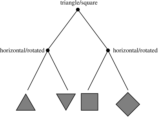
FIG. 2.: An example for a decision tree. Two binary choices have to be made to identify the shape (triangle or square) and the orientation (horizontal or rotated). In sending with equal probability one of the four objects, one therefore transmits 2 bits of information.

B Information is physical

In the previous subsection we have introduced the concept of the bit as the unit of information. In the course of the argument we mentioned already that information can be encoded in physical systems. In fact, looking at it more closely, we realize that any information is encoded, processed and transmitted by physical means. Physical systems such as capacitors or spins are used for storage, sound waves or optical fibers for transmission and the laws of classical mechanics, electrodynamics or quantum mechanics dictate the properties of these devices and limit our capabilities for information processing. These rather obvious looking statements, however, have significant implications for our understanding of the concept of information as they emphasize that the theory of information is not a purely mathematical concept, but that the properties of its basic units are dictated by the laws of physics. The different laws that rule in the classical world and the quantum world for example results in different information processing capabilities and it is this insight that sparked the interest in the general field of quantum information theory.

In the following we would like to further corroborate the view that information and physics should be unified to a physical theory of information by showing that the process of erasure of information is invariably accompanied by the generation of heat and that this insight leads to a resolution of the longstanding Maxwell demon paradox which is really a prime example of the deep connection between physics and information. The rest of the article will then attempt to apply the connection between erasure of information and physical heat generation further to gain insight into recent results in quantum information theory.

C Erasing classical information from classical systems: Landauer’s principle

We begin our investigations by concentrating on classical information. In 1961, Rolf Landauer had the important insight that there is a fundamental asymmetry in the way Nature allows us to process information [12]. Copying classical information can be done reversibly and without wasting any energy, but when information is erased there is always an energy cost of $kTln2$ per classical bit to be paid. For example, as shown in fig. 3, we can encode one bit of information in a binary device composed of a box with a partition.

FIG. 3.: We erase the information of the position of the atom. First we extract the wall separating the two halves of the box. Then we use a piston to shift the atom to the left side of the box. After the procedure, the atom is on the left hand side of the box irrespective of its intial state. Note that the procedure has to work irrespective of whether the atom is initially on the right (figure (a)) or on the left side (figure (b)).

The box is filled with a one molecule gas that can be on either side of the partition, but we do not know which one. We assume that we erase the bit of information encoded in the position of the molecule by extracting the partition and compressing the molecule in the right part of the box irrespective of where it was before. We say that information has been erased during the compression because we will never find out where the molecule was originally. Any binary message encoded is lost! The physical result of the compression is a decrease in the thermodynamical entropy of the gas by $kln2$. The minimum work that we need to do on the box is $kTln2$, if the compression is isothermal and quasi-static. Furthermore an amount of heat equal to $kTln2$ is dumped in the environment at the end of the process.

Landauer’s conjectured that this energy/entropy cost cannot be reduced below this limit irrespective of how the information is encoded and subsequently erased - it is a fundamental limit. In the discussion of the Maxwell demon in the next section we will see that this principle can be deduced from the second law of thermodynamics and is in fact equivalent to it [22]. Landauer’s discovery is important both theoretically and practically as on the one hand it relates the concept of information to physical quantities like thermodynamical entropy and free energy and on the other hand it may force the future designers of quantum devices to take into account the heat production caused by the erasure of information although this effect is tiny and negligible in today’s technology.

At this point we are ready to summarize our findings on the physics of classical information.

1) Information is always encoded in a physical system.

2) The erasure of information causes a generation of $kTln2$

of heat per bit in the environment.

Armed with this knowledge we will present the first successful application of the erasure principle: the solution of the Maxwell’s demon paradox that has plagued the foundations of thermodynamics for almost a century.

D Maxwell’s demon deposed

1 The paradox

In this section we present a simplified version of the Maxwell’s demon paradox suggested by Leo Szilard in 1929 [23]. It employs an intelligent being or a computer of microscopic size, operating a heat engine with a single molecule working fluid (figure 4).

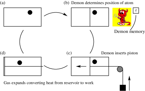
FIG. 4.: A schematical picture of Szilard’s engine of a box filled with a one atom gas. Initially the position of the atom is unknown. Then the demon measures the position and depending on the outcome inserts a piston. Then the gas expands and thereby does work on a load attached to the piston. This procedure is repeated and we apparently do work at the sole expense of extracting heat from one reservoir only.

In this scheme, the molecule is originally placed in a box, free to move in the entire volume V as shown in step (a). Step (b) consists of inserting a partition which divides the box in two equal parts. At this point the Maxwell’s demon measures in which side of the box the molecule is and records the result (in the figure the molecule is pictured on the right-hand side of the partition as an example). In step (c) the Maxwell demon uses the information to replace the partition with a piston and couple the latter to a load. In step (d) the one-molecule gas is put in contact with a reservoir and expands isothermically to the original volume $V$. During the expansion the gas draws heat from the reservoir and does work to lift the load. Apparently the device is returned to its initial state and it is ready to perform another cycle whose net result is again full conversion of heat into work, a process forbidden by the second law of thermodynamics.

Despite its deceptive simplicity, the argument above has missed an important point: while the gas in the box has returned to its initial state, the mind of the demon hasn’t! In fact, the demon needs to erase the information stored in his mind for the process to be truly cyclic. This is because the information in the brain of the demon is stored in physical objects and cannot be regarded as a purely mathematical concept! The first attempts to solve the paradox had missed this point completely and relied on the assumption that the act of acquisition of information by the demon entails an energy cost equal to the work extracted by the demonic engine, thus preventing the second law to be defeated. This assumption is wrong! Information on the position of the particle can be acquired reversibly without having to pay the energy bill, but erasing information does have a cost! This important remark was first made by Bennett in a very readable paper on the physics of computation [14]. We will analyze his argument in some detail. Bennett developed Szilard’s earlier suggestion [23] that the demon’s mind could be viewed as a two-state system that stores one bit of information about the position of the particle. In this sense, the demon’s mind can be an inanimate binary system which represents a significant step forward, as it rids the discussion from the dubious concept of intelligence. After the particle in the box is returned to the initial state the bit of information is still stored in the demon’s mind (ie in the binary device). Consequently, this bit of information needs to be erased to return the demon’s mind to its initial state. By Landauer’s principle this erasure has an energy cost

$$W_{erasure}=-kTln2\;.$$ (1)

On the other hand, the work extracted by the demonic engine in the isothermal expansion is

$$W_{extracted}=+kTln2\;.$$ (2)

All the work gained by the engine is needed to erase the information in the demon’s mind, so that no net work is produced in the cycle. Furthermore, the erasure transfers into the reservoir the same amount of heat that was drawn from it originally. So there is no net flow of heat either. There is no net result after the process is completed and the second law of thermodynamics is saved! The crucial point in Bennett’s argument is that the information processed by the demon must be encoded in a physical system that obeys the laws of physics. The second law of thermodynamics states that there is no entropy decrease in a closed system that undergoes a cyclic transformation. Therefore if we let the demon measure the Szilard’s engine we need to include the physical state he uses to store the information in the analysis, otherwise there would be an interaction with the environment and the system would not be closed. One could also view the demon’s mind as a heat bath initially at zero temperature. After storing information in it, the mind appears to an outside observer like a random sequence of digits and one could therefore say that the demons mind has been heated up. Having realized that the demon’s mind is a second heat bath, we now have a perfectly acceptable process that does not violate the second law of thermodynamics.

2 Generalized entropy

The solution of the paradox presented in the last section views the ”brain of the demon” as a physical system to be included in the entropy balance together with the box that is being observed (see part (b) of figure 5).

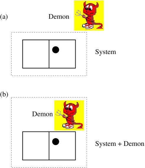
FIG. 5.: A figure that shows the two different viewpoints discussed in this section. The demon is outside the system which consists of the box and the atom only (figure (a)) or the demon and the box form a joint system that is closed.

A different approach can be taken if one does not want to consider explicitly the workings of the demon’s mind, but just treat it as an external observer that obtains information about the system (see part (a) of figure 5). This is done by including in the definition of the entropy of the system a term that represents the knowledge that the demon has on the state of the system together with the well known term representing how ordered the state is [24, 13].

In the context of Szilard’s engine we found that the demon extracts from the engine an amount of work given by

$$W_{extracted}=kTln2=\Delta Q=T\Delta S,$$ (3)

where $\Delta S$ is the change of thermodynamical entropy in the system when the heat $\Delta Q$ is absorbed from the environment. On the other hand, to erase his memory he uses at least an equal amount of work given by

$$W_{erasure}=-kTln2=-TI,$$ (4)

where $I$ denotes the information required by the demon to specify on which side of the box the molecule is times the scaling factor $kln2$. In this case the information is just 1 bit. The scaling factor is introduced for consistency because the definition of information is given in bits as a logarithm in basis 2 of the number of memory levels in the demon’s mind.

The total work gained (equal to the total heat exchanged $Q_{total}$ since the system is kept at constant temperature T) is thus given by

$$W_{total}=W_{erasure}+W_{extracted}=Q_{total}=T(\Delta S-I)=0\;.$$ (5)

This suggests that the second law of thermodynamics is not violated if we introduce a generalized definition of entropy $\Im$ (in bits) as the difference of the thermodynamical entropy of the system $\Delta S$ and the information about the system $I$ possessed by an external observer.

$$\Im=\Delta S-I\;.$$ (6)

The idea of modifying the definition of thermodynamical entropy that represents an objective property of the physical system with an ”informational term” relative to an external observer appears bizarre at first sight. Physical properties like entropy identify and distinguish physical states. By introducing a notion as information directly in the second law of thermodynamics we somehow bolster the view that an ensemble composed of partitioned boxes each containing a molecule in a position unknown to us is not the same physical state than an ensemble in which we know exactly on which side of the partition the molecule is in each box. Why? Because we can extract work from the second state by virtue of the knowledge we gained, but we cannot do the same with the first. We will encounter similar arguments in later sections when we study the concept of information in the context of quantum theory. For the time being, we remark that the approach presented in this section to the solution of the Maxwell’s demon paradox adds new meaning to the slogan information is physical. Information is physical because it is always encoded in a physical system and also because the information we possess about a physical system contributes to define the state of the system.

E The information content of a classical state in bits

So far we have discussed how information is encoded in a classical system and subsequently erased from it. However, we really haven’t quantified the information content of a complicated classical system composed of many components each of which can be in one of $n$ states with probability $p_{n}$. This problem is equivalent to determining the information content of a long classical message. In fact, a classical message is encoded in a string of classical objects each representing a letter from a known alphabet occurring with a certain probability. The agreed relation between objects and letters represents the required background knowledge for communication. Bob sends this string of objects to Alice. She knows how the letters of the alphabet are encoded in the objects, but she does not know the message that Bob is sending. When Alice receives the objects, she can decode the information in the message, provided that none of the objects has been accidentally changed on the way to her. Can we quantify the information transmitted if we know that each letter $\rho_{i}$ occurs in the message with probability $p_{i}$? Let us begin with some hand-waving which is followed in the next section by a formally correct argument. Assume that our alphabet is composed of only two letters $1$ and $0$ occurring with probability $p_{1}=0.1$ and $p_{0}=0.9$ respectively. Suppose we send a very long message, what is the average information sent per letter? Naively, one could say that if each letter can be either $1$ or $0$ then the information transmitted per letter has to be $1$ bit. But this answer does not take into account the different probabilities associated with receiving a $1$ or a $0$. For example, presented with an object Alice can guess its identity in $90\%$ of the cases by simply assuming it is $0$. On the other hand, if the letters $1$ and $0$ come out with equal probability, she will guess correctly only $50\%$ of the time. Therefore her surprise will usually be bigger in the second case as she doesn’t know what to expect. Let us quantify Alice’s surprise when she finds letter $i$ which normally occurs with probability $p_{i}$ by

$$\mbox{surprise letter i}=log\frac{1}{p_{i}}\;.$$ (7)

We have chosen the logarithm of $\frac{1}{p_{i}}$ because if we guess two letters, then the surprise should be additive, i.e.

$$\log(\frac{1}{p_{i}}\frac{1}{p_{j}}) = \log\frac{1}{p_{i}}+\log\frac{1}{p_{j}}\;\;.$$ (8)

$$= \mbox{surprise letter i}+\mbox{surprise letter j}\;\;.$$ (9)

and this can only be satisfied by the logarithm. Now we can compute the average surprise, which we find to be given by the Shannon entropy

$$H=\sum_{i}p_{i}\log\frac{1}{p_{i}}=-\sum_{i}p_{i}\log p_{i}\;.$$ (10)

This argument is of course hand-waving and therefore the next section addresses the problem more formally by asking how much one can compress a message, i.e. how much redundancy is included in a message.

1 Shannon’s entropy

In $1948$ Shannon developed a rigorous framework for the description of information and derived an expression for the information content of the message which indeed depends on the probability of each letter occurring and results in the Shannon entropy. We will illustrate Shannon’s reasoning in the context of the example above. Shannon invoked the law of large numbers and stated that, if the message is composed of $N$ letters where $N$ is very large, then the $typical$ messages will be composed of $Np_{1}$ 1’s and $Np_{0}$ 0’s. For simplicity, we assume that $N$ is 8 and that $p_{1}$ and $p_{0}$ are $\frac{1}{8}$ and $\frac{7}{8}$ respectively. In this case the typical messages are the $8$ possible sequences composed of 8 binary digits of which only one is equal to $1$ (see left side of figure 6).

FIG. 6.: The idea behind classical data compression. The most likely sequences are relabeled using fewer bits while rare sequences are discarded. The smaller number of bits still allows the reconstruction of the original sequences with very high probability.

As the length of the message increases (i.e. $N$ gets large) the probability of getting a message which is all 1’s or any other message that differs significantly from a typical sequence is negligible so that we can safely ignore them. But how many distinct typical messages are there? In the previous example the answer was clear: just $8$. In the general case one has to find in how many ways the $Np_{1}$ 1’s can be arranged in a sequence of N letters? Simple combinatorics tells us that the number of distinct typical messages is

$$\left(\begin{array}[]{c}N\\ Np_{1}\end{array}\right)=\frac{N!}{(Np_{1})!(Np_{0})!}$$ (11)

and they are all equally likely to occur. Therefore, we can label each of these possible messages by a binary number. If that is done, the number of binary digits $I$ we need to label each typical message is equal to $log_{2}\frac{N!}{Np_{1}!Np_{0}!}$. In the example above each of the 8 typical message can be labeled by a binary number composed by $I=log_{2}8=3$ digits (see figure 6). It therefore makes sense that the number $I$ is also the number of bits encoded in the message, because Alice can unambiguously identify the content of each typical message if Bob sends her the corresponding binary number, provided they share the background knowledge on the labeling of the typical messages. All other letters in the original message are really redundant and do not add any information! When the message is very long almost any message is a typical one. Therefore, Alice can reconstruct with arbitrary precision the original $N$ bits message Bob wanted to send her just by receiving $I$ bits. In the example above, Alice can compress an 8 bits message down to 3 bits. Though, the efficiency of this procedure is limited when the message is only 8 letters long, because the approximation of considering only typical sequences is not that good. We leave to the reader to show that the number of bits $I$ contained in a large $N$-letter message can in general be written, after using Stirling’s formula, as

$$I=-N(p_{1}logp_{1}+p_{0}logp_{0})\;.$$ (12)

If we plug the numbers $\frac{1}{8}$ and $\frac{7}{8}$ for $p_{0}$ and $p_{1}$ respectively in equation 12, we find that the information content per symbol $\frac{I}{N}$ when N is very large is approximately $0.5436$ bits. On the other hand, when the binary letters 1 and 0 appear with equal probabilities, then compression is not possible, i.e. the message has no redundancy and each letter of the message contains one full bit of information per symbol. These results match nicely the intuitive arguments given above.

Equation 12 can easily be generalized to an alphabet of $n$ letters $\rho_{i}$ each occurring with probabilities $p_{i}$. In this case, the average information in bits transmitted per symbol in a message composed of a large number $N$ of letters is given by the Shannon entropy:

$$\frac{I}{N}=H\{p_{i}\}=-\sum_{i=1}^{n}p_{i}logp_{i}\;.$$ (13)

We remark that the information content of a complicated classical system composed of a large number $N$ of subsystems each of which can be in any of $n$ states occurring with probabilities $p_{i}$ is given by $N\times H\{p_{i}\}$.

2 Boltzmann versus Shannon entropy

The mathematical form of the Shannon entropy $H$ differs only by a constant from the entropy formula derived by Boltzmann after counting how many ways are there to assemble a particular arrangement of matter and energy in a physical system.

$$S=-kln2\sum_{i=1}^{n}p_{i}logp_{i}\;.$$ (14)

To convert one bit of classical information in units of thermodynamical entropy we just need to multiply by $kln2$. By Landauer’s erasure principle, the entropy so obtained is the amount of thermodynamical entropy you will generate in erasing the bit of information.

Boltzmann statistical interpretation of entropy helps us to understand the origin of equation 6. Consider our familiar example of the binary device in which the molecule can be on either side of the partition with equal probabilities. An observer who has no extra knowledge will use Boltzmann’s formula and work out that the entropy is $kln2$. What about an observer who has 1 extra bit of information on the position of the molecule? He will use the Boltzmann’s formula again, but this time he will use the values $1$ and $0$ for the probabilities, because he knows on which side the molecule is. After plugging these numbers in equation 14, he will conclude that the entropy of the system is $0$ in agreement with the result obtained if we use equation 6. The acquisition of information about the state of a system changes its entropy simply because the entropy is a measure of our ignorance of the state of the system as transparent from Boltzmann’s analysis.

F Sending classical information through a noisy classical channel

In the previous section, we found that the Shannon entropy measures the information content in bits of an arbitrary message whose letters are encoded in classical objects. Throughout our discussion, we made an important assumption: that the message is encoded and transmitted to the recipient without errors. It is obvious that this situation is quite unrealistic. In realistic scenarios communication errors are unavoidable. To the physicist eyes, the origin of noise in communication can be traced all the way down to the unavoidable interaction between the environment and the physical systems in which each letter is encoded. The errors caused by the noise in the communication channel cannot be eliminated completely. However, one hopes to devise a strategy that enables the recipient of the message to detect and subsequently correct the errors, without having to go all the way to the sender to check the original message. This procedure is sometimes referred to as coding the original message.

1 Coding a classical message: an example

For example, imagine that Bob wants to send to Alice a $1$ bit message encoded in the state of a classical binary device in which a particle can be on the left hand side (encode a $0$) or the right hand side (encode a $1$) of a finite potential barrier. Unfortunately, the system is noisy and there is a probability $\frac{1}{100}$ for the binary letter to flip (i.e. $1\rightarrow 0$ or $0\rightarrow 1$). For example, a thermal fluctuation induced by the environment may cause the particle in the encoding device to overcome the potential barrier and go from the left hand side to the right hand side. Alice, who is not aware of this change, will therefore think that Bob attempted to send a $1$ and not a $0$. This event occurs with $1\%$ probability so it is not that rare after all. On the other hand, the (joint) probability that two such errors occur in the same message is only $0.01\%$ ($\frac{1}{100}\times\frac{1}{100}$). Alice and Bob decide to ignore the unlikely event of two errors happening in one encoding but they still want to protect their message against single errors. How can they achieve this?

One strategy is to add extra digits to the original message and dilute the information contained in it among all the binary digits available in the extended message. Here is an example. Alice and Bob add two extra digits. Now their message is composed of $3$ binary digits, but they still want to get across only one bit of information. So they agree that Alice will read a $1$ whenever she receives the sequence $111$ and a $0$ when she receives $000$.

The reader can see that this encoding ensures safer communication, because the worst that can happen is that Alice receives a message in which not all the digits are either 0s or 1s, for example $101$. But that is not big deal. In this case the original message was clearly a $111$, because we have allowed for single errors only. Under this assumption, any original message of the form $000$ can never get transformed in $101$ because that requires flipping at least two bits.

This strategy protects the message from single errors and therefore ensures that the error rate in the communication is reduced down to 0.01% (the probability of double errors). By simply adding other two extra bits to the encoded message Bob can protect the message against double errors and reduce the error rate of two orders of magnitude (ie the probability of triple errors). Quite obviously one can make the error rate as small as possible but at the price of decreasing the ratio of $\frac{\mbox{bits transmitted}}{\mbox{binary letters employed}}$. Is it possible to achieve a finite ratio $\frac{\mbox{bits transmitted}}{\mbox{binary letters employed}}$ and an arbitrarily small error rate in the decoded messages? We will address this question, that has been first answered by Shannon, in the next section.

2 The capacity of a noisy classical channel via Landauer’s principle

Maybe surprisingly, one can indeed bring the error rate in the received message in communication arbitrary close to zero, provided that the actual message of length $N$ bits is ”coded” in a much longer message of size $N_{C}$ bits. The actual construction of efficient strategies to code a message is a task that requires a lot of ingenuity, but is not what we are after. Our concern here is to answer the following more fundamental question:

Given that the probability of error is $q$, what is the largest number of bits $N$ that we can transmit reliably through a noisy channel after encoding them in a larger message of size $N_{C}$ bits?

In other words we want a bound on the classical information capacity of a noisy channel. We start by remarking that if the coded message is composed of $N_{C}$ bits, then the average number of errors will be $qN_{C}$. If we let the size of the message be very large, the probability of getting a number of errors different from the average value becomes vanishing small. In the asymptotic limit one will expect exactly $qN_{C}$ bits to be affected by errors in the $N_{C}$ bits message. However, there are many ways in which $qN_{C}$ errors can be distributed in the $N_{C}$ bits of the original message. In fact, we worked out the exact number in the section on the Shannon entropy and it is given by

$$\mbox{number of ways the errors can be distributed}=\left(\begin{array}[]{c}N_{C}\\ qN_{C}\end{array}\right)\;.$$ (15)

The problem there was slightly different, but after rephrasing the argument a bit we can conclude that in order to specify how the $qN_{C}$ errors are distributed among the $N_{C}$ message bits you need $n$ bits of information, where $n$ is given by :

$$n = \log\left(\begin{array}[]{c}N_{C}\\ qN_{C}\end{array}\right)\cong-N_{C}[qlogq+(1-q)log(1-q)]$$ (18)

$$= N_{C}H(q).$$ (19)

The reader should convince himself that equation 19 can be derived following the same steps that led us to equation 12. One just needs to rename the variables.

The short calculation above may inspire the following idea. Bob can send only $N_{C}$ bits in total and he knows that he needs $N_{C}H(q)$ bits to specify the position of the errors. All he has to do, then, is to allocate $N_{C}H(q)$ binary digits to store the information on the position of the errors. At that point the remaining $N_{C}-N_{C}H(q)$ binary digits will be fully available for safe communication. Unfortunately, Bob cannot implement this idea directly because it requires him to know, in advance, which letters of the message are going to be affected by errors. But the errors are random and they would occur even in the letters that supposedly store information on their positions! But there is something to be learned from this suggestion anyway.

Suppose, instead, that Bob had diluted the information he wants to transmit among all the letters of the message as shown in the last section. When Alice receives the string of binary digits and she deciphers the message, she gains knowledge of the actual message, but also the information necessary to extract the message from all the digits. This extra amount of information is implicitly provided by the coding technique and it is also diluted among all the letters in the message. To see this point more clearly, let us use Landauer’s principle and ask how much entropy Alice generates when she decides to erase the message sent by Bob. For simplicity, let us stick to our simple example where Bob sends $3$ bits to effectively transmit only a $1$ bit message. In order to erase the information sent by Bob, Alice has to reset to zero the three classical binary devices sent by Bob and that generates an amount of entropy not less than $3kln2$, by Landauer’s principle. But, Alice has effectively acquired only 1 bit of information corresponding to $kln2$ of entropy. So why did she have to generate that extra amount of entropy equal to $2kln2$? Those extra 2 bits of information that she is erasing must have been implicitly used to identify the errors and separate them from the real message. In general, when Alice receives the string of $N_{C}$ binary devices and she erases it, the minimum amount of entropy that she generates is equal to $N_{C}\times kln2$. Now we can figure out how much of that entropy needs to be wasted to extract the real message from these (redundant) string of binary digits. No matter how sophisticated Bob’s coding was, there is no way that Alice could isolate the errors without using at least $N_{C}H(q)$ bits of information. In fact, even if she can compress the errors in a block of digits and concentrate the message in the remaining block she would still need at least $N_{C}H(q)$ binary digits for the errors. Note that we are by no means proving that she will be able to achieve this efficiency, but only that she will compress the errors in a block of at least $N_{C}H(q)$ binary letters. But, if Alice and Bob could device such a strategy, something much more sophisticated than the naive idea suggested above, then they would really have $N_{C}-N_{C}H(q)$ bits available for error free communication. That means that there is an upper bound on the information capacity of any classical noisy channel given by

$$N=N_{C}(1-H(q))$$ (20)

where $N$ is the size of the message effectively transmitted, $N_{C}$ is the size of the (larger) coded message and $q$ is the probability that each bit will flip under the effect of the noise. The rigorous proof that this bound is indeed achievable was given by Shannon (see textbooks such as [21]). The reader interested in more details can consult the Feynman lectures on computation on which this short treatment was based [18].

The problem of the noisy channel concludes our survey of classical information encoded in classical systems. If you have a look at the map of this paper you will see that we have gone through one of the 4 columns of topics shown pictorially in figure 1. The rest of this paper will deal with topics that require a grasp of the basic principles and mathematical methods of quantum mechanics. The next section is a quick recap that should be of help to those with a more limited background. If the reader feels confident in the use of the basics of quantum mechanics, the density operator and tensor products, then he can just skip this part and move on to the next section.

III A crash course on quantum mechanics

At the end of our discussion on the Maxwell’s demon paradox, we started putting forward the idea that the information we have on the state of a classical system contributes to define the state itself. In this section we will push our arguments even further and investigate the role that the concept of information plays in the basic formalism of quantum mechanics.

A To be or to know

The quantum state of a physical system is usually represented mathematically by a vector $|\psi\rangle$ or a matrix ${\hat{\rho}}$ in a complex vector space called the Hilbert space [15, 16, 17, 19]. We will explain the rules and the reasoning behind this representation in the next sections by considering two-level quantum systems as an easy example that displays most of the features of the general case.

But, first of all, what do the mathematical symbols exactly represent? In this article, we take the pragmatic point of view that what is being represented is not the quantum system itself but rather the information that we have about its preparation procedure. As an example that illustrates this point, we consider the process by which an atom prepared in an arbitrary superposition of energy eigenstates collapses into only one of the eigenstates after the measurement is done. This process seems to happen instantaneously unlike the ordinary time evolution of quantum states. Generations of physicists have been puzzled by this fact and have searched for the physical mechanism which causes the collapse of the wave function. However, if we consider the wave-function to represent only the information that we possess about the state of the quantum system, we will definitely expect it to change discontinuously after the measurement has taken place, because our knowledge has suddenly increased. Not everybody is satisfied with this view. Some people think that physical theories should deal with objective properties of Nature, with what is really out there and avoid subjectivism. It is difficult to assess the validity of these arguments entirely on philosophical grounds. To our knowledge there are no experiments that provide compelling evidence in favor of any of the existing interpretational frameworks. Therefore we will adopt what we feel is the easiest way out of the problem and explain the rules for representing mathematically our knowledge of the preparation procedure of an arbitrary quantum state [25].

B Pure states and complete knowledge

1 Pure states of a single system

We start by considering how to proceed when we have complete knowledge on the preparation procedure of a single quantum system. In this simpler case, we say that the state of the quantum system is pure and we represent our complete knowledge of its preparation procedure as a vector in a complex vector space. As an example, consider two non-orthogonal states of a two-level atom $|\psi_{1}\rangle$ and $|\psi_{0}\rangle$. These states are arbitrary superpositions of the two energy eigenstates. In the next few lines, we show how to write them as two $2$-dimensional vectors

$$|\psi_{1}\rangle = \frac{2}{\sqrt{5}}|0\rangle+\frac{1}{\sqrt{5}}|1\rangle\;\;.$$ (21)

$$= \frac{2}{\sqrt{5}}\left(\begin{array}[]{c}1\\ 0\end{array}\right)+\frac{1}{\sqrt{5}}\left(\begin{array}[]{c}0\\ 1\end{array}\right)\;\;.$$ (26)

$$= \frac{1}{\sqrt{5}}\left(\begin{array}[]{c}2\\ 1\end{array}\right)\;\;.$$ (29)

$$|\psi_{0}\rangle = \frac{1}{\sqrt{2}}|0\rangle+\frac{1}{\sqrt{2}}|1\rangle\;\;.$$ (30)

$$= \frac{1}{\sqrt{2}}\left(\begin{array}[]{c}1\\ 1\end{array}\right)\;\;.$$ (33)

The rule used above to convert from Dirac to matrix notation is to write the energy eigenstates $|0\rangle$ and $|1\rangle$, as the column vectors $\left(\begin{array}[]{c}1\\ 0\end{array}\right)$ and $\left(\begin{array}[]{c}0\\ 1\end{array}\right)$, respectively. There is nothing mystical behind the choice of this correspondence. One could have also chosen the basis vectors $\frac{1}{\sqrt{2}}\left(\begin{array}[]{c}1\\ 1\end{array}\right)$ and $\frac{1}{\sqrt{2}}\left(\begin{array}[]{c}-1\\ 1\end{array}\right)$, instead. What is important is that the two vectors are $orthogonal$ and normalized so that they can faithfully represent the important $experimental$ property that the two states $|0\rangle$ and $|1\rangle$ are orthogonal and can be perfectly $distinguished$ in a measurement. The important point to observe in the choice of the basis in which to represent your state-vectors is that of consistency. Every physical quantity has to be represented in the same basis when you bring them together in computations. If one has used different bases for representation, then one has to rotate them into one standard basis using unitary transformations. This rotation can be expressed mathematically as $2\times 2$ unitary matrix $U$. A unitary matrix is defined by the requirement that $UU^{\dagger}=U^{\dagger}U={\bf 1}$. Given a set of quantities in one basis then upon rewriting them in another basis, the predictions for all physically observable quantities have to remain the same. This essentially requires that the mathematical expressions that are used to express these observable quantities have to be invariant under unitary transformations. We will see examples of this soon.

Above we have seen examples for orthogonal states (namely the basis states $|0\rangle$ and $|1\rangle$, as the column vectors $\left(\begin{array}[]{c}1\\ 0\end{array}\right)$ and $\left(\begin{array}[]{c}0\\ 1\end{array}\right)$ ). In general two quantum states will be neither orthogonal nor parallel such as for example the states $|\psi_{0}\rangle$ and $|\psi_{1}\rangle$. To quantify the angle between two vectors $|\psi_{i}\rangle$ and $|\psi_{j}\rangle$ we introduce the complex scalar product. For complex vectors with two components it is given by

$$\langle\psi_{j}|\psi_{i}\rangle = ({a_{j}}^{*}\langle 0|+{b_{j}}^{*}\langle 1|)(a_{i}|0\rangle+b_{i}|1\rangle)\;\;.$$ (34)

$$= \left(\begin{array}[]{c c}{a_{j}}^{*}&{b_{j}}^{*}\end{array}\right)\left(\begin{array}[]{c}a_{i}\\ b_{i}\end{array}\right)\;\;.$$ (38)

$$= {a_{j}}^{*}a_{i}+{b_{j}}^{*}b_{i}\;\;.$$ (39)

Note that the components of the first vector have to be complex conjugated, but apart from that the complex scalar product behaves just as the ordinary real scalar product. One nice property of the scalar product is the fact that it is invariant under unitary transformations, just as you would expect for a quantity that measures the angle between two state vectors.

2 Operators and probabilities for a single system

In our new language of state vectors, the dot product $\langle\psi_{i}|\psi_{j}\rangle$ is analogous to the overlap integral between two wave-functions $\psi_{i}(x)$ and $\psi_{j}(x)$, that is usually encountered in introductory courses of quantum mechanics. The reader may recall that the squared result of the overlap integral, write as ${|\langle\psi_{i}|\psi_{j}\rangle|}^{2}$, can be interpreted as the probability of projecting the quantum state $|\psi_{i}\rangle$ on the eigenstate $|\psi_{j}\rangle$ of an appropriate observable after the measurement is performed.

Now we would like to represent this projection mathematically by a projection operator denoted by $|\psi\rangle\langle\psi|$. This projector is simply a matrix that maps all the vectors onto the vector corresponding to $|\psi_{j}\rangle$, apart from a normalization constant. The recipe to construct the matrix representation of $|\psi\rangle\langle\psi|$ is to multiply the column vector $|\psi\rangle$ times the row vector $\langle\psi|$ as shown below:

$$|\psi\rangle\langle\psi| = (a|0\rangle+b|1\rangle)(a^{*}\langle 0|+b^{*}\langle 1|)\;\;.$$ (40)

$$= \begin{array}[]{c}\\ \left(\begin{array}[]{c}a\\ b\end{array}\right)\\ \end{array}\begin{array}[]{c}\left(\begin{array}[]{c c}{a}^{*}&{b}^{*}\end{array}\right)\\ \\ \\ \end{array}$$ (49)

$$= \left(\begin{array}[]{c c}|a|^{2}&a{b}^{*}\\ {a}^{*}b&|b|^{2}\end{array}\right)\;\;.$$ (52)

For example, the reader can easily construct the matrix representing the projector $|1\rangle\langle 1|$ and check that when it operates on the state $|\psi_{0}\rangle$ in equation 33 we indeed obtain the excited state $|1\rangle$ apart from a normalization constant. Furthermore, the probability of finding the state $|\psi\rangle$ in a measurement of a system originally in the quantum state $|\phi\rangle$ is given by

$$Prob_{|\psi\rangle}=\langle\phi|(|\psi\rangle\langle\psi|)|\phi\rangle=tr\{|\psi\rangle\langle\psi||\phi\rangle\langle\phi|\}$$ (53)

where $tr$ denotes the trace which is the sum of the diagonal elements of a matrix, a concept that is invariant under unitary transformations. The reader can easily check that Eq. 53 is true by explicitly constructing the matrices $|\psi\rangle\langle\psi|$ and $|\phi\rangle\langle\phi|$ (see equation 52), multiplying them, take the trace, and verify that the result is indeed equal to $|\langle\phi|\psi\rangle|^{2}$, calculated after squaring the result of equation 39. Once this is done it is easy to write the expectation value of any observable whose eigenvalues are the real numbers $\{e_{i}\}$ and its eigenstates are the vectors $\{|e_{i}\rangle\}$. In fact, if we label the probability of projecting on the eigenstate $|e_{i}\rangle$ as $Prob_{|e_{i}\rangle}$ and we make use of equation 53, we can indeed write the expectation value for any observable ${\hat{O}}$ of the two level system in a given state $|\phi\rangle$ as

$$\langle{\hat{O}}\rangle_{|\phi\rangle} = e_{0}Prob_{|e_{0}\rangle}+e_{1}Prob_{|e_{1}\rangle}\;\;.$$ (54)

$$= e_{0}tr\{|e_{0}\rangle\langle e_{0}||\phi\rangle\langle\phi|\}+e_{1}tr\{|e_{1}\rangle\langle e_{1}||\phi\rangle\langle\phi|\}\;\;.$$ (55)

$$= tr\{(e_{0}|e_{0}\rangle\langle e_{0}|+e_{1}|e_{1}\rangle\langle e_{1}|)|\phi\rangle\langle\phi|\}\;.$$ (56)

The expression above can be tided up a bit by defining the observable ${\hat{O}}$ as the matrix

$${\hat{O}}=e_{0}|e_{0}\rangle\langle e_{0}|+e_{1}|e_{1}\rangle\langle e_{1}|\;.$$ (57)

Note that in order to use the projectors to calculate probabilities as in equation 56, we have to demand that the sum of the matrices representing the projectors must be the unity matrix. For a two dimensional vector space this means that $|0\rangle\langle 0|+|1\rangle\langle 1|=1$. This condition ensures that the sum of the probabilities obtained using equation 56 is equal to $1$. Once we check this important property of the projectors we can use equation 57 to construct the matrix representation of any observable. For example, the reader can check that the energy observable ${\hat{E}}$ can be written using the basis $\left(\begin{array}[]{c}1\\ 0\end{array}\right)$ and $\left(\begin{array}[]{c}0\\ 1\end{array}\right)$ in the form:

$${\hat{E}} = e_{0}|e_{0}\rangle\langle e_{0}|+e_{1}|e_{1}\rangle\langle e_{1}|\;\;.$$ (58)

$$= e_{0}\left(\begin{array}[]{c c}1&0\\ 0&0\end{array}\right)+e_{1}\left(\begin{array}[]{c c}0&0\\ 0&1\end{array}\right)\;\;.$$ (63)

$$= \left(\begin{array}[]{c c}e_{0}&0\\ 0&e_{1}\end{array}\right)\;\;.$$ (66)

Note that the energy operator is diagonal in this basis because these basis vectors were originally chosen as the energy eigenvectors! However, the prescription given in equation 57 to represent any observable ${\hat{O}}$ ensures that the resulting matrix is Hermitian because the projectors themselves are Hermitian. A matrix is said to be Hermitian if all its entries that are symmetrical with respect to the principal diagonal are complex conjugate of each other (see equation 52). The fact that the matrix ${\hat{O}}$ is Hermitian ensures that its eigenvectors are orthogonal and the corresponding eigenvalues are real. This means that the possible ”output states” after the measurement are distinguishable and the corresponding results are real numbers. Once you accept equation 57, you can immediately write equation 56 simply as

$$\langle{\hat{O}}\rangle=tr\{{\hat{O}}|\psi_{i}\rangle\langle\psi_{i}|\}$$ (67)

This completes our quick survey of the rules to represent the arbitrary state of a single two level quantum system. The main motivation to adopt these rules is dictated by their ability to correctly predict experimental results.

3 Non-orthogonality and inaccessible information

We would like to expand a little bit on the important concept of non-distinguishibility between two quantum states. By this we mean the following. Suppose that you are given two two-level atoms in states $|\psi_{0}\rangle$ and $|\psi_{1}\rangle$ respectively (see equations 33 and 29) and you are asked to work out which particle is in state $|\psi_{1}\rangle$ and which in state $|\psi_{0}\rangle$. The two states are said to be non-distinguishable if you will never be able to achieve this task without the possibility of a wrong answer and if you are given only one system and irrespective of the observable you to measure. For example you could decide to measure the energy of the two atoms. After using equation 53or just by inspection, you can verify that the probability of finding the atom in the excited state if it was in state $|\psi_{0}\rangle$ before the measurement is equal to $\frac{1}{5}$. On the other hand, you can also check that the probability of finding the atom in the excited state if it was in state $|\psi_{1}\rangle$ before the measurement is also non-vanishing and in fact equal to $\frac{1}{2}$. Now, suppose that you perform the measurement and you find that the atom is indeed in the excited state. At this point, you still cannot unambiguously decide whether the atom had been prepared in state $|\psi_{0}\rangle$ or $|\psi_{1}\rangle$ before the measurement took place. In fact, by measuring any other observable only once you will never be able to distinguish between two non-orthogonal states with certainty.

This situation is somehow surprising because the two non-orthogonal states are generated by different preparation procedures. Information was invested to prepare the two states, but when we try to recover it with a single measurement we fail. The information on the superposition of states in which the system was prepared remains not accessible to us in a single measurement.

It is sometimes argued that we therefore have to assume that a single quantum mechanical measurement does not give us any information. This viewpoint is, however, wrong. Consider the situation above again, where we either have the state $|\psi_{0}\rangle$ or the state $|\psi_{1}\rangle$ with a priori probabilities $1/2$ each. If we find in a measurement the excited state of the atom, then it would be a fair guess to say that it is more likely that the system was in state $|\psi_{1}\rangle$ because this state has the higher probability to yield the excited state in a measurement of the energy. Therefore the a posteriori probability distribution for the two states has changed, and therefore we have gained knowledge as we have reduced our uncertainty about the identity of the quantum state.

The non-distinguishability of non-orthogonal quantum states is an important aspect of quantum mechanics and will be encountered again several times in the remainder of this article.

4 Two 2-level quantum systems in a joint pure state

We have gained a good grasp of the properties of an isolated two-level quantum system. We are now going to study how the joint quantum state of two such systems (say a pair of two level atoms) is represented mathematically. The generalization is straightforward. We initially concentrate on the situation when our knowledge of the preparation procedure of the joint state is complete, i.e. when the joint system is in a pure state. The reader who is not very familiar with quantum mechanics may wonder why we have to include this section altogether. At the end of the day, according to classical intuition, the state of a joint quantum system comprised of two subsystems $A$ and $B$ can be given by simply providing, at any time, the state of each of the subsystems $A$ and $B$ independently. This reasonable conclusion turns out to be wrong in many cases! Let us see why.

We first consider one of the most intuitive examples of joint state of the two atoms: the case in which atom $A$ is in its excited state $|1\rangle_{A}$ and atom $B$ in its ground state $|0\rangle_{B}$, where the subscript labels the atoms and the binary number their states. In this case, the joint state of the two atoms $|\psi_{AB}\rangle$ can be fully described by stating the state of each atom individually so we write $|\psi_{AB}\rangle$ down symbolically as $|1\rangle_{A}$ $|0\rangle_{B}$. We call this state a product state. We now decide to represent the joint state $|1\rangle_{A}|0\rangle_{B}$ of the two atoms as a vector in an enlarged Hilbert space whose dimensionality is no longer $2$ as for a single atom but it is $2\times 2=4$. The vector representation of $|1\rangle_{A}|0\rangle_{B}$ is constructed as shown below:

$$|\psi_{AB}\rangle = |1\rangle_{A}|0\rangle_{B}$$ (68)

$$= \left(\begin{array}[]{c}0\\ 1\end{array}\right)\otimes\left(\begin{array}[]{c}1\\ 0\end{array}\right)$$ (73)

$$:= \left(\begin{array}[]{c}0\times 1\\ 0\times 0\\ 1\times 1\\ 1\times 0\end{array}\right)$$ (78)

$$= \left(\begin{array}[]{c}0\\ 0\\ 1\\ 0\end{array}\right)\;\;.$$ (83)

Equation 83 defines the so called tensor product between two vectors belonging to two different Hilbert spaces, one used to represent the state of atom A and the other for atom B. For the readers who have never seen the symbol $\otimes$ we write down a more general case involving the two vectors $|\psi_{A}\rangle$ with coefficients $a$ and $b$ and $|\psi_{B}\rangle$ with coefficients $c$ and $d$:

$$|\psi_{AB}\rangle = |\psi_{A}\rangle|\psi_{B}\rangle$$ (84)

$$= \left(\begin{array}[]{c}a\\ b\end{array}\right)\left(\begin{array}[]{c}c\\ d\end{array}\right)$$ (89)

$$:= \left(\begin{array}[]{c}ac\\ ad\\ bc\\ bd\end{array}\right)\;\;.$$ (94)

The case of tensor product between $n$ dimensional vectors is a simple generalization of the rule of multiplying component-wise as above [16]. Using equation 94 the reader can work out the vector representation of the following states:

$$|0\rangle_{A}|0\rangle_{B}\longrightarrow\left(\begin{array}[]{c}1\\ 0\\ 0\\ 0\end{array}\right),$$ (95)

$$|0\rangle_{A}|1\rangle_{B}\longrightarrow\left(\begin{array}[]{c}0\\ 1\\ 0\\ 0\end{array}\right),$$ (96)

$$|1\rangle_{A}|1\rangle_{B}\longrightarrow\left(\begin{array}[]{c}0\\ 0\\ 0\\ 1\end{array}\right).$$ (97)

A trick to write the states above as vectors without explicitly performing the calculation in equation 83 is the following. First, read the two digits inside $|...\rangle|...\rangle$ as two digits binary numbers (for example read $|0\rangle|1\rangle$ as 1), and add $1$ to get the resulting number $n$. Then place a $1$ in the $n^{th}$ entry of the column vector and 0s in all the others. The four states-vectors in equations 83, 95, 96 and 97 are a complete set of orthogonal basis vectors for our four-dimensional Hilbert space. Therefore, any state $|\psi_{AB}\rangle$ of the form $|\psi_{B}\rangle|\psi_{A}\rangle$ in equation 94 can be written as:

$$|\psi_{AB}\rangle=ac|0\rangle_{A}|0\rangle_{B}+ad|0\rangle_{A}|1\rangle_{B}+bc|1\rangle_{A}|0\rangle_{B}+bd|1\rangle_{A}|1\rangle_{B}.$$ (98)

where we wrote the vectors symbolically, in Dirac notation, to save paper. We interpret the coefficients of each basis vector in terms of probability amplitudes, as we did for single systems. For example, the modulus squared $|ad|^{2}$ gives the probability of finding atom $A$ in its ground state and atom $B$ in the excited state after an energy measurement. A question that arises naturally after inspecting equation above is the following:

What happens when I choose the coefficients of the superposition in equation 98 in such a way that it is impossible to find two vectors $|\sigma\rangle_{A}$ and $|\beta\rangle_{B}$ that ”factorize” the 4-dimensional vector $|\psi_{AB}\rangle$ as in equation 94? Are these non factorizable vectors a valid mathematical representation of quantum states that you can actually prepare in the lab?

5 Bipartite Entanglement

The answer to the previous question is a definite yes. Before expanding on this point, let us write an example of a non factorizable vector:

$$|\psi_{AB}\rangle=\frac{1}{\sqrt{2}}|0\rangle_{A}|0\rangle_{B}+\frac{1}{\sqrt{2}}|1\rangle_{A}|1\rangle_{B}.$$ (99)

The vector above corresponds to the state for which there is equal probability of finding both atoms in the excited state or both in the ground state. The reader can perhaps make a few attempts to factorize this vector, but they are all going to be unsuccessful. This vector, nonetheless, represents a perfectly acceptable quantum state. In fact, according to the laws of quantum mechanics, ANY vector in the enlarged Hilbert space is a valid physical state for the joint system of the two atoms, independently of it being factorizable or not. In fact, in section V B 2 we will show that for an $n$-partite system most of the states are actually non factorizable. So these states are the norm rather than the exception!

The existence of non-factorizable states is not too difficult to appreciate mathematically, but it leads to some unexpected conceptual conclusions. If the quantum state of a composite system cannot be factorized than it is impossible to specify a pure state of its constituent components. More strangely perhaps, non-factorizable states, such as $|\psi_{AB}\rangle$ in equation 99 are pure states. This means that the corresponding vectors are mathematical representations of our complete knowledge of their preparation procedure. There is nothing more we can in principle know about these composite quantum objects than what we have written down, but nonetheless we still cannot have full knowledge of the state of their subsystems. With reference to the discussion following equation 99, we conclude that in a non-factorizable state we have knowledge of the correlation between measurements outcomes on atom $A$ and $B$ but we cannot in principle identify a pure state with each of the atoms $A$ and $B$ individually. This phenomena seemed very weird to the fathers of quantum mechanics who introduced the name entangled states to denote states whose corresponding vectors cannot be factorized in the sense explained above. In section VI, that is entirely devoted to this topic, we will go beyond the dry mathematical notion of non-factorizability and start exploring the physical properties that make entangled states peculiar. We will focus on possible applications of these weird quantum objects in the lab. But before doing that, the reader will have to swallow another few pages of definition and rules because we have not explained yet how to construct and manipulate operators acting on our enlarged Hilbert space.

6 Operators and probabilities for two systems

In this section, we generalize the discussion of projection operators and observables given previously for single quantum systems to systems consisting of two particles. The generalization to $n$-particle systems should then be obvious. We start by asserting that the rules stated in equations 53 and 57 for single quantum systems are still valid with the only exception that now observables and projector operators are represented by $4\times 4$ matrices. Imagine that you want to write down the joint observable ${\hat{O}}_{A}\otimes{\hat{O}}_{B}$ where ${\hat{O}}_{A}$ and ${\hat{O}}_{B}$ are possibly different observables acting respectively on the Hilbert space of particle A and of particle B. The rule to write down the joint observable is the following:

$${\hat{O}}_{AB} = {\hat{O}}_{A}\otimes{\hat{O}}_{B}\;\;.$$ (100)

$$= \left(\begin{array}[]{c c}a_{1}&b_{1}\\ c_{1}&d_{1}\end{array}\right)\otimes\left(\begin{array}[]{c c}a_{2}&b_{2}\\ c_{2}&d_{2}\end{array}\right)\;\;.$$ (105)

$$= \left(\begin{array}[]{c c c c}a_{1}a_{2}&a_{1}b_{2}&b_{1}a_{2}&b_{1}b_{2}\\ a_{1}c_{2}&a_{1}d_{2}&b_{1}c_{2}&b_{1}d_{2}\\ c_{1}a_{2}&c_{1}b_{2}&d_{1}a_{2}&d_{1}b_{2}\\ c_{1}c_{2}&c_{1}d_{2}&d_{1}c_{2}&d_{1}d_{2}\end{array}\right)\;\;.$$ (110)

where the subscript $1$ denotes the operator on particle $A$ and the subscript $2$ the operator on particle $B$. However, there are some observables ${\hat{O}_{AB}}$ whose corresponding matrices cannot be factorized as in equation 110. These matrices still represent acceptable observables provided that they are Hermitian.

Furthermore, it is possible to construct projectors on any $4d$ vectors by using the same principle illustrated in equation 52. For example, the projector on the entangled state $|\psi\rangle_{AB}$ in equation 99 can be written as

$$|\psi_{AB}\rangle\langle\psi_{AB}| = \frac{1}{2}\left(\begin{array}[]{c}1\\ 0\\ 0\\ 1\end{array}\right)\left(\begin{array}[]{c c c c}1&0&0&1\end{array}\right)\;\;.$$ (116)

$$= \frac{1}{2}\left(\begin{array}[]{c c c c}1&0&0&1\\ 0&0&0&0\\ 0&0&0&0\\ 1&0&0&1\end{array}\right)\;\;.$$ (121)

Finally, suppose you are interested in knowing the probability of projecting atom A on its ground state $|0\rangle_{A}$ and atom B onto its excited state $|1\rangle_{B}$ after performing a measurement on the maximally correlated state $|\psi_{AB}\rangle$ considered above. How do you proceed? The answer to this question should be of guidance also for other cases, so we work it out in some detail. The first thing you do is to construct the tensor product of the matrices corresponding to the single particle projectors $|0\rangle\langle 0|$ and $|1\rangle\langle 1|$ that project particle A onto its ground state and particle B on its excited state:

$$|0\rangle\langle 0|\otimes|1\rangle\langle 1| = \left(\begin{array}[]{c c}1&0\\ 0&0\end{array}\right)\otimes\left(\begin{array}[]{c c}0&0\\ 0&1\end{array}\right)\;\;.$$ (126)

$$= \left(\begin{array}[]{c c c c}0&0&0&0\\ 0&1&0&0\\ 0&0&0&0\\ 0&0&0&0\end{array}\right)\;\;.$$ (131)

Once you have worked out the matrix in equation 131 you can multiply it with the matrix found in equation 121 and take the trace, as explained for single particles in equation 53. The result is 0, as expected, since we have maximal correlations between the two atoms in state $|\psi_{AB}\rangle$.

C Mixed states and incomplete knowledge

1 Mixed states of a single two-level atom

In this section, we explain how to represent mathematically the state of a quantum system whose preparation procedure is not completely known to us. This lack of knowledge may be caused by random errors in the apparatus that generates our quantum systems or by fluctuations induced by the environment. In these cases we say that the quantum system is in a mixed state. This can be contrasted with the pure states considered in the previous sections for which there was no lack of knowledge of the preparation procedure (i.e. the quantum states were generated by a perfect machine whose output was completely known to us). To some extent, by considering mixed states, we start dealing with ”real world quantum mechanics”. We will build on the example introduced in section III B 1 to make our treatment more accessible.

An experimentalist needs to prepare two-level atoms in the state $|\psi_{1}\rangle$ to be subsequently used in an experiment. He has at his disposal an oven that generates atoms in the state $|\psi_{1}\rangle$ with probability $p_{1}=95\%$ (see Fig. 7 for illustration).

FIG. 7.: An oven emits atomic two-level systems. The internal state of the system is randomly distributed. With probability $p_{i}$ the system is in the pure state $|\psi_{i}\rangle$. A person oblivious to this random distribution measures observable ${\hat{A}}$. What is the mean value that he obtains?

In the remaining $p_{0}=5\%$ of the cases the oven fails and generates atoms in a different state $|\psi_{0}\rangle$. This preparation procedure is pretty efficient, but of course still different from the ideal case. The experimentalist collects the atoms, but he does not know for which of them the preparation has been successful because the experimental errors occur randomly in the oven. Neither can he measure the atoms because he is scared of perturbing their quantum state. The only thing he knows is the probability distribution of the two possible states. The experimentalist has to live with this uncertainty. However, he his aware that, if he uses the states produced by the oven, his experimental results are going to be different from the ones he would have obtained had he used atoms in the state $|\psi_{1}\rangle$ exactly, because the oven occasionally outputs atoms in the undesired state $|\psi_{0}\rangle$. He would like to find an easy way to compute the measurement results in this situation so he asks a theorist to help him modeling his experiments. The first task the two have to face is to construct a mathematical object that represents their incomplete knowledge of the preparation procedure. Intuitively, it cannot be the vector $|\psi_{1}\rangle$ because of that $5\%$ probability of getting the state $|\psi_{0}\rangle$. The way the two approach the problem is a good example of empirical reasoning, so it is worth exploring their thought process in some detail. The theorist asks the experimentalist to describe what he needs to do with these atoms and the two reach the conclusion that what really matters to them are the expectation values of arbitrary observables measured on the states generated by the oven. The theorist points out that, after performing measurements on $N$ atoms, the experimentalist will have used, approximately, $Np_{1}$ atoms in the state $|\psi_{1}\rangle$ and $Np_{0}$ atoms in state $|\psi_{0}\rangle$. For each of the two states $|\psi_{i}\rangle$ they would know how to calculate the expectation value for any observable ${\hat{A}}$ that the experimentalist wants to measure. After using equation 57 the theorist rewrites the expectation value of the observable ${\hat{A}}$ on the state $|\psi_{i}\rangle$ as $tr\{{\hat{A}}|\psi_{i}\rangle\langle\psi_{i}|\}$. The two are now only one step away from the result. What they need to do is to average the two expectation values for the states $|\psi_{1}\rangle$ and $|\psi_{0}\rangle$ with the respective probabilities. The mean value observed by the experimentalist is thus given by:

$$\langle{\hat{A}}\rangle = \sum_{i}p_{i}tr\{{\hat{A}}|\psi_{i}\rangle\langle\psi_{i}|\}$$ (132)

$$= tr\{{\hat{A}}\sum p_{i}|\psi_{i}\rangle\langle\psi_{i}|\}\;\;.$$ (133)

The calculation above can be tided up a bit by defining the density operator ${\hat{\rho}}$ as

$${\hat{\rho}}=\sum p_{i}|\psi_{i}\rangle\langle\psi_{i}|\;\;.$$ (134)

Once this is done equation 133 can be compactly written as

$$\langle{\hat{A}}\rangle=tr\{{\hat{A}}{\hat{\rho}}\}\;\;.$$ (135)

A glance at these few lines of mathematics convinces the two physicists that they have actually solved their problem. In fact the density operator is the mathematical description of the knowledge the two have about the quantum states prepared by the oven. Equation 135, on the other hand, tells them exactly how to use their knowledge to compute the expectation value of any operator.

Similarly, they can write down the probability of finding the system in any state $|\sigma\rangle$ after a measurement by simply constructing the projector $|\sigma\rangle\langle\sigma|$. After this, they just multiply it with the density operator and take the trace (as in equation 53)

$$Prob_{|\sigma\rangle}=tr\{|\sigma\rangle\langle\sigma|{\hat{\rho}}\}\;\;.$$ (136)

Equation 134 provides the recipe for constructing the density matrix for the example above. We leave as an exercise to the reader to show that the density operator representing the preparation procedure described above can be written as

$${\hat{\rho}}=\left(\begin{array}[]{c c}0.785&0.405\\ 0.405&0.215\\ \end{array}\right)$$ (137)

One can see that the trace of the density operator ${\hat{\rho}}$ in equation 137 is equal to $1$. This is not an accident but a distinctive property of any density operator. You can easily check that by plugging the unity matrix rather than the operator ${\hat{O}}$ in equation 135. The expectation value of the unity operator on any normalized vector state is $1$ (i.e. the expectation value reduces to the dot product of the normalized state vector with itself). That in turn implies via equation 135 that the trace of ${\hat{O}}$ is $1$.

To sum up, one can use density operators in matrix form to represent both states of complete and incomplete knowledge (i.e. pure or mixed states). We saw, however, that for pure states a vector representation is sufficient. If one wants to use the same mathematical tool to write down any state irrespective of the knowledge he holds on its preparation procedure then the method of choice is the density operator (also called density matrix). A system is in a pure state when the corresponding density operator in equation 134 contains only one term. In this ideal case, there is no lack of knowledge on the preparation of the system, the preparation procedure generates the desired output with unit probability. This implies that the diagonalized density matrix representing a pure state has all entries equal to zero except one entry equal to $1$ on the principal diagonal. Therefore, if you take the trace of the diagonalized density matrix squared, you will still get one. Furthermore, the trace of the diagonalized density matrix squared is equal to the trace of the original density matrix squared (remember the trace is invariant under unitary transformations). This observation is the basis of a criterion to check whether a given density matrix represents a pure or a mixed state. The test consists in taking the trace of the density matrix squared. If the trace is equal to $1$, then the state is pure otherwise it is mixed. We recall that a mixed state arises in situation when the preparation procedure is faulty and the result is a distribution of different outputs each occurring with a given probability.

2 Mixed states for two quantum systems

Our treatment of density operators for single quantum systems can be applied to bipartite systems with no essential modification. Let us consider an example in which an experimental apparatus produces the maximally entangled state $|\psi_{AB}\rangle$ (see equation 99) with probability $p_{0}$ and the product state $|0\rangle_{A}|0\rangle_{B}$ with probability $p_{1}$. For both states we know how to construct the corresponding projectors by using the same method illustrated in equation 121. But, before writing down the resulting density operator, we introduce a small simplification in the notation used. We write the state $|0\rangle_{A}|0\rangle_{B}$ simply as $|00\rangle_{AB}$ or simply $|00\rangle$. The rule to write down the four-dimensional vector corresponding to this state and its interpretation does not change. The first digit still refers to atom $A$ and the second to atom $B$. We can now write the corresponding density operator ${\hat{\rho}_{AB}}$ as shown in equation 134

$${\hat{\rho}_{AB}} = p_{0}|\psi_{AB}\rangle\langle\psi_{AB}|+p_{1}|00\rangle\langle 00|\;\;$$ (138)

$$= \frac{p_{0}}{2}\left(\begin{array}[]{c c c c}0&0&0&0\\ 0&1&1&0\\ 0&1&1&0\\ 0&0&0&0\end{array}\right)+p_{1}\left(\begin{array}[]{c c c c}1&0&0&0\\ 0&0&0&0\\ 0&0&0&0\\ 0&0&0&0\end{array}\right)\;\;$$ (147)

$$= \left(\begin{array}[]{c c c c}p_{1}&0&0&0\\ 0&\frac{p_{0}}{2}&\frac{p_{0}}{2}&0\\ 0&\frac{p_{0}}{2}&\frac{p_{0}}{2}&0\\ 0&0&0&0\end{array}\right)\;.$$ (152)

There is another situation that will arise in later sections. Suppose that two distant machines are generating one atom each, but we do not know exactly the preparation procedure of each atom. Since the two machines are very far away from each other, we can ignore the interaction between the atoms and describe them separately in two different 2-dimensional Hilbert spaces by writing down the corresponding single particle density operators ${\hat{\rho}_{A}}$ and ${\hat{\rho}_{B}}$. All this is fine. But, we may also write the joint state of these two non-interacting atoms as a density operator ${\hat{\rho}_{AB}}$ in our 4-dimensional Hilbert space, as we did for the case considered in equation 152. How do we proceed? We simply take the tensor product between the two $2\times 2$ matrices corresponding to ${\hat{\rho}_{A}}$ and ${\hat{\rho}_{B}}$ to get

$${\hat{\rho}_{AB}}={\hat{\rho}_{A}}\otimes{\hat{\rho}_{B}}$$ (153)

We leave as an exercise for the reader to choose two arbitrary density operators ${\hat{\rho}_{A}}$ and ${\hat{\rho}_{B}}$ and perform an explicit calculation of ${\hat{\rho}_{AB}}$.

Once we know how to write 1) the density matrix for the joint state of the two atoms and 2) the matrix representing a joint observable or projector we will have no trouble finding expectation values or probabilities of certain measurement outcomes. All we need to do is to multiply two $4\times 4$ matrices and take the trace as illustrated for a single particle in equations 135 and 136.

3 The reduced density operator

There is another context in which a mixed state arises even when there is no uncertainty in the preparation procedure of the quantum system one is holding. Imagine you have an ideal machine that generates, with probability one, pairs of maximally entangled particles in the state $|\psi_{AB}\rangle=\frac{1}{\sqrt{2}}(|00\rangle+|11\rangle)$. The density operator $\rho_{AB}$ for this pure state reduces to the corresponding projector, because all the probabilities except one are vanishing see discussion at the end of section III C 1. In fact, the $4\times 4$ density matrix for this preparation procedure was explicitly calculated in equation 121.

After having created the entangled pair we decide to lock particle $A$ in a room to which we have no access and we give particle $B$ to our friend Bob. Bob can do any measurement he wants on particle $B$ and he would like to be able to predict the outcomes of any of these. Evidently Bob does not know what is happening to particle A after it has been locked away and as a consequence now he has an incomplete knowledge of the total state. The question is how we can describe mathematically his state given the incomplete knowledge that Bob has of particle $A$. The first point to make is that Bob still has some background knowledge on particle $A$ because he retains information on the original preparation procedure of the entangle pair. For example, he knows that if Alice subjects her particle to an energy measurement and finds that particle $A$ is in the ground (excited) state, then particle B has to be in the ground (excited) state too. This prediction is possible because the measurement outcomes of the two particles are always correlated because they were prepared in the entangled state $|\psi_{AB}\rangle$. Furthermore, Bob knows from the preparation procedure, that the probability that Alice finds her particle in either the ground state $|0\rangle_{A}$ or in the excited state $|1\rangle_{A}$ is $\frac{1}{2}$. By using the non local correlations between his particle and the other, Bob concludes that particle $B$ too is in either the ground state $|0\rangle_{B}$ or in the excited state $|1\rangle_{B}$ with probability $\frac{1}{2}$. Now let us assume that Alice indeed has measured the energy operator on her particle but, as she is inside the box, has not told Bob that she did this. Therefore, in half the cases Bob’s particle will be in state $|0\rangle\langle 0|$ and in half the cases it will be in state $|1\rangle\langle 1|$. This is a situation that is most easily described by a density operator. We find that the state of Bob’s particle is described by the reduced density operator ${\hat{\rho}_{B}}$ given by:

$${\hat{\rho}_{B}} = \frac{1}{2}|0\rangle\langle 0|+\frac{1}{2}|1\rangle\langle 1|\;\;.$$ (154)

$$= \frac{1}{2}\left(\begin{array}[]{c c}1&0\\ 0&1\end{array}\right)\;\;.$$ (157)

where we used the rules for the representation and manipulation of quantum states as vectors (equation 52). From the above reasoning it is perhaps not surprising that ${\hat{\rho}_{B}}$ is often termed the reduced density operator. Being a mixed state, it represents Bob’s incomplete information on the state of his particle (the reduced system) due to his inability to access particle A while the total system is in a pure entangled state represented by the larger matrix ${\hat{\rho}_{AB}}$. In fact, Bob wrote down ${\hat{\rho}_{B}}$ after taking into account all information that was available to him. It is important to note that we would have obtained the same result for Bob’s density operator if we had assumed any other operation on Alice’s side. The key point is that, as Alice’s actions do not affect Bob’s particle in any physically detectable way, it should not make any difference for Bob’s description of his state which assumptions he makes for Alice’s action.

The whole operation of ignoring Alice’s part of the system and generating a reduced density operator only for Bob’s system is sometimes written mathematically as

$${\hat{\rho}_{A}}=tr_{B}\{{\hat{\rho}_{AB}}\}\;.$$ (158)

The mathematical operations that one has to perform on the entries of the larger matrix ${\hat{\rho}_{AB}}$ in order to obtain ${\hat{\rho}_{A}}$ are called the partial trace over system B. The general case can be dealt with analogously to the reasoning above. One assumes that in the inaccessible system a measurement is carried out whose outcomes are not revealed to us. We then determine the state of our system for any specific outcome from the projection postulate and we use the associated probabilities to form the appropriate density operator. We refer the reader interested in learning how to deal with this method in the most efficient way to some recent courses of quantum mechanics [16, 17, 15].

This topic concludes our very concise review of quantum mechanics. We will now extensively apply the mathematical tools introduced in this section to deal with situations in which classical information is encoded in a quantum system and later to discuss the new field of quantum information theory. It is therefore essential that the reader feels confident with what he has learned so far before moving on.

IV Classical information encoded in quantum systems

A How many bits can we encode in a quantum state?

In the previous section, we studied two situations in which the state of a quantum system is mixed, namely when the preparation procedure is not completely known or when we have a subsystem that is part of a larger inaccessible system. In both cases, our knowledge was limited to the probabilities $\{p_{i}\}$ that the system is in one of the pure states $|\psi_{i}\rangle$. A question that arises naturally in this context is whether we can assign an entropy to a quantum system in a mixed state in very much the same way as we do with a classical system that can be in a number of distinguishable configurations with a given set of probabilities. In the classical case the answer is the well known Boltzmann formula given in equation 14. At first sight, you may think that the same formula can be applied to evaluate the mixed state entropy just by plugging in the probabilities $\{p_{i}\}$ that the quantum system is in one of the pure quantum states $|\psi_{i}\rangle$. Unfortunately, this idea does not work, because the quantum states $|\psi_{i}\rangle$ are different from the distinguishable configuration of a classical system in one important way. They are not always perfectly distinguishable! As we pointed out earlier, two quantum states can be non-orthogonal and therefore not perfectly distinguishable. But maybe the idea of starting from the classical case as a guide to solve our quantum problem is not that bad after all.

In particular, imagine that you are given the density matrix representing the mixed state of a quantum system. Can you perform some mathematical operations on this matrix to bring it in a form that is more suggestive? You may recall from equations 52 and 134 that the procedure to write down this density matrix is the following. First construct the matrix representation of the projector $|\psi_{i}\rangle\langle\psi_{i}|$ for each of the vectors $|\psi_{i}\rangle$, then multiply each of them by their respective probability and finally sum all up in one matrix. The reader can check that the prescription on how to construct each matrix $|\psi_{i}\rangle\langle\psi_{i}|$ given in equation 52 ensures that the resulting density matrix is Hermitian. We denote the orthogonal eigenvectors of our (hermitian) density matrix by $|e_{i}\rangle$. If we choose the $|e_{i}\rangle$ as basis vectors, we can rewrite our matrix in a diagonal form. All the entries on the diagonal are the real eigenvalues of the matrix. These matrices can now be written in Dirac notation as

$${\hat{\rho}}=\sum q_{i}|e_{i}\rangle\langle e_{i}|\;\;,$$ (159)

where the $q_{i}$ are now the eigenvalues of the density matrix. This new matrix actually represents another preparation procedure namely the mixed state of a quantum system which can be in any of the $orthogonal$ states $|e_{i}\rangle$ with probability $q_{i}$. But now the states $|e_{i}\rangle$ are distinguishable and therefore one can apply the Boltzmann formula by simply plugging the eigenvalues of the matrix as the probabilities.

There is one problem in this reasoning. When you rewrite the old density matrix in diagonal form you are actually writing down a different matrix and therefore a representation of a different preparation procedure. How can you expect then that the entropy so found applies to the mixed state you considered originally? The answer to this question lies in the fact that what matters in the matrix representation of quantum mechanical observables or states is not the actual matrix itself, but only those properties of the matrix that are directly connected to what you can observe in the lab. From the previous section, we know that all the physically relevant properties are basis independent. The diagonalization procedure mentioned above is nothing else than a change of basis and therefore there is no harm in reducing our original density matrix $\hat{\rho}$ in diagonal form and hence define the von Neumann entropy as the function

$$S({\hat{\rho}}) = -tr\{{\hat{\rho}}log{\hat{\rho}}\}\;\;$$ (160)

$$= -\sum q_{i}\log q_{i}\;\;.$$ (161)

The formula above is an example of how a function of a matrix can be evaluated as an ordinary function of its eigenvalues only. Since the eigenvalues are invariant under a change of basis the function itself is invariant, as expected. One can check the validity of the formula above as an entropy measure by considering two limiting cases. Consider first a pure state, for which there is no uncertainty on the output of the preparation procedure. The probability distribution reduces to only one probability which is one. Therefore the density matrix representing this state has eigenvalue equal to one. If you plug the number one in the logarithm in formula 161 you get the reassuring result that the entropy of this state is zero. On the other hand, for a maximally mixed state in which the system can be prepared randomly in one of $N$ equally likely pure state we find that the entropy is $logN$ in agreement (in dimensionless units) with the Boltzmann and Shannon entropies.

There is an interesting point to note. If we create a mixed state by generating the states $\{|\psi_{i}\rangle\}$ with probabilities $\{p_{i}\}$ we first hold a list of numbers which tell us which system is in which quantum state. In this classical list each letter holds $H(\{p_{i}\})$ bits of information. If we want to complete the creation of the mixed states, we have to erase this list and, according to Landauer’s principle, will generate $kTH(\{p_{i}\})$ of heat per erased message letter. In general the Shannon entropy is larger than or equal to the von Neumann entropy of the density operator $\hat{\rho}=\sum_{i}p_{i}|\psi_{i}\rangle\langle\psi_{i}|$. It is also clear that the same mixed state can be created in many different ways and that the information invested into the state will not be unique. It seems therefore unclear whether we can ascribe a unique classical information content to a mixed state. However, the only quantity that is independent of the particular way in which the mixed state has been generated is the von Neumann entropy which is different from the amount of information invested in the creation of the mixed state. In fact, the von Neumann entropy $S(\hat{\rho})$ is the smallest amount of information that needs to be invested to create the mixed state $\hat{\rho}$. As we are unable to distinguish different preparations of the same density operator ${\hat{\rho}}$ this is certainly the minimum amount of classical information in the state $\hat{\rho}$ that we can access. The question is whether we can access even more classical information. The answer to this question is $NO$, as we will see in the next section in which we generalize Landauers principle to the quantum domain to illuminate the situation further. The result of these considerations is that there is a difference between information that went into a mixed state, and the accessible information that is left after the preparation of the states [19].

B Erasing classical information from quantum states: Landauer’s principle revisited

In the previous subsection we have discussed the amount of classical information that goes into the creation of a mixed state. But an obvious question has not been discussed yet: how do you erase the classical information encoded in a quantum mixed state ? In section II C, we explained how to erase one bit encoded in a partitioned box filled with a one molecule gas. All you have to do in this simple case is to remove the partition and compress the gas on one side of the box (say the right) independently of where it was before. This procedure erases the classical state of the binary device and the bit of information encoded in it. If the compression is carried out reversibly and at constant temperature, then the total change of thermodynamical entropy is given by $kln2$, the minimum amount allowed by Landauer’s principle. In this sense the erasure is optimal. What we are looking for in this section is a procedures for the erasure of the state of quantum systems. We will first present a direct generalization of the classical erasure procedure and then follow this up with a more general procedure that applies directly to both classical and quantum systems. These results will then be used to show that the accessible information in a quantum state $\hat{\rho}$ created from an ensemble of pure states is equal to $S(\hat{\rho})$.

1 Erasure involving measurement

We know from the previous section that the information content of a pure state is zero. Therefore, all we need to do to erase the information encoded in a mixed quantum state, is to return the system to a fixed pure state called the standard state. We show how to achieve this in the context of an example.

Imagine you want to erase the information encoded in quantum systems in the mixed state $\rho=\sum_{i}p_{i}|e_{i}\rangle\langle e_{i}|$ where the $|e_{i}\rangle$ are the energy eigenstates. You start by performing measurements in the energy eigenbasis . After the measurement is performed, each system will indeed be in one of the pure states $|e_{i}\rangle$ and we have a classical record describing the measurement outcomes. If the density operator represents the preparation procedure of two level atoms and we measure their energies, the classical measurement record would be a set of partitioned boxes storing a list of 0s and 1s labeling the energy of the ground state or the excited state for each atom measured. Now we can apply a unitary transformation and map the state $|e_{i}\rangle$ onto the standard state $|e_{0}\rangle$ for each atom on which a measurement has been performed (see first step in figure 8).

FIG. 8.: Particles described by a quantum state $\rho$ arrive and are being measured in a basis $|e_{i}\rangle$ giving the outcome $i$ with probability $p_{i}$. Given the outcome the each of the particles can be rotated into the pure state $|e_{0}\rangle$. The remaining classical list has to be erased as well. This generates $kTln2H(\{p_{i}\})$ of heat. This procedure can be optimized if one measures in the eigenbasis of $\rho$ in which case one generates $kTln2S(\rho)$ heat.

Naively, one could think that this completes the erasure, because we have reset the quantum systems to a fixed standard state $|e_{0}\rangle$. However this is not true, because we are still holding the classical measurement records so the erasure is still not complete. We need one more step namely to erase the classical measurement record using the classical procedure discussed above. In the example of figure 8 , this amounts to compressing each of the partitioned boxes where the list of 0s and 1s were encoded. This process will generate an amount of thermodynamical entropy not less than $kln2$ per bit. In general we have that $k\ln 2S(\hat{\rho})\leq k\ln 2H(p)$ as pointed out in the previous section. The optimal erasure procedure, ie the one that creates the least amount of heat, is the one where the quantum measurements are made in the basis of the eigenstates of $\hat{\rho}$, so that the Shannon entropy equals the von Neumann entropy as discussed in section IV A .

To sum up, the protocol described above relies on a quantum mechanical measurement followed by a unitary transformation and the erasure of the classical measurement record. While this protocol is a perfectly acceptable erasure procedure, it consists of two conceptually different steps and one may wonder whether there is a simpler method that does not involve the explicit act of measuring the quantum system.

2 Erasure by thermal randomization

Such an elegant way to erase information, which has been introduced by Lubkin [38, 40], is by thermal randomization. Simply stated, you have to place the quantum system that is to be erased into contact with a heat bath at temperature $T$. The laws of statistical mechanics teach us that when thermal equilibrium is reached, there will be an uncertainty about the energy state the system is in. The origin of this uncertainty is classical because it is induced by thermal fluctuations. This situation of lack of knowledge of the preparation procedure for the quantum state is equivalent to the example of the oven considered in section III C 1. The state of the system can therefore be written as a density operator ${\hat{\omega}}$ given by

$${\hat{\omega}} = \frac{e^{-\beta{\hat{H}}}}{Z}$$ (162)

$$= \frac{\sum_{i}e^{-\beta{E_{i}}}|e_{i}\rangle\langle e_{i}|}{Z}\;\;,$$ (163)

where $\beta=1/kT$, ${\hat{H}}$ is the Hamiltonian of the system whose eigenstates and eigenvalues are $|e_{i}\rangle$ and $E_{i}$ respectively. The number $Z$ is the partition function of the system and can be calculated from $Z=tr\{e^{-\beta{\hat{H}}}\}$. For example, the system can be in its ground state with probability $p_{0}$ given by the Boltzmann distribution:

$$\ p_{0}=\frac{e^{-\beta E_{0}}}{Z}\;\;.$$ (164)

The exponential dependence of the probabilities in the equation above implies that, if the system has a sufficiently large level spacing (ie $E_{0}$ is much smaller than the other energy levels), it will be almost surely in its ground state. Thus, if a measurement is made, the result will be almost certainly that the apparatus is in its ground state. In other words, the mixed state ${\hat{\rho}}$ can be made arbitrarily close to a standard pure state $|e_{0}\rangle$ by greatly reducing the presence of the other pure states $|e_{i}\rangle$ in the thermal preparation procedure. In practice, this is exactly what we wanted: a procedure that always resets our system, originally in the mixed state ${\hat{\rho}}$, to a standard state (independent of the initial state), eg the ground state $|e_{0}\rangle$. Also note that this erasure procedure never requires any measurement to be performed, so we do not need to be concerned with erasing the classical measurement record, as in the previous method.

Furthermore, we can readily calculate the net amount of thermodynamical entropy generated in erasing the quantum mixed state ${\hat{\rho}}$ where the classical information is encoded. We proceed by computing first the change of thermodynamical entropy in the system and then the change of thermodynamical entropy of the environment. All the steps in this derivation are reproduced and motivated. The readers who do not feel comfortable with the formalism of density operators explained in the previous sections can skip this derivation and jump to the result in equation 173.

The mixed state $\hat{\rho}$ is generated by a source that produces randomly pure states $|e_{i}\rangle$ with probability $p_{i}$. Each quantum system in such a pure state $|e_{i}\rangle$ is brought into contact with the heat bath and thermalizes into the state $\hat{\omega}$ (see figure 9).

FIG. 9.: The quantum particles, described by the average state $\rho$, are brought into contact with a thermal heat bath and are allowed to relax into thermal equilibrium. The resulting change of heat depends on the temperature of the heat bath and its optimal value is given by $kTln2S(\rho)$

We remind the reader that the entropy of the system before the thermalization procedure takes place is zero because the system is in one of the pure states $|e_{i}\rangle$ (see equation 161 and discussion below). Therefore, in each of these contacts, the thermodynamical entropy of the system increases by the same amount $kln2S(\hat{\omega})$, where $S(\hat{\omega})$ is the von Neumann entropy times the conversion factor between information and thermodynamical entropy, so that we have

$$\Delta S_{sys}=kln2S(\hat{\omega})\;.$$ (165)

Now we proceed to discuss the change in the thermodynamical entropy of the heat bath. The latter is given in terms of the heat lost by the heat bath and its temperature $T$ by the well known thermodynamical relation $\Delta S_{bath}=\frac{\Delta Q_{bath}}{T}$. The easiest way to attack this problem is by using the observation that the change of heat in the heat bath $\Delta Q_{bath}$ is equal and opposite to the change of heat in the system $\Delta Q_{system}$. The latter is given in terms of the heat lost by the system and the temperature of the reservoir by the well known thermodynamical relation $T\Delta S_{system}=\Delta Q_{system}$. Furthermore, the first law of thermodynamics can be used to write $\Delta Q_{system}$ as the change in the internal energy of the system $\Delta U_{system}=U_{final}-U_{initial}$ (i.e. the procedure can be done reversibly so that the work required is arbitrary close to $0$). One can summarize what is stated above in the equation:

$$\Delta S_{bath}=-\frac{\Delta U_{system}}{T}=-\frac{U_{final}-U_{initial}}{T}\;.$$ (166)

We can now rewrite the initial and final energy of the system as the expectation value of the Hamiltonian ${\hat{H}}$ of the system calculated in the initial state ${\hat{\rho}}$ and in the final thermal state ${\hat{\omega}}$. The formula to use is given in equation 135. Once this is done equation 166 can be recast in the following form:

$$\Delta S_{bath} = -\frac{tr\{{\hat{\omega}}{\hat{H}}\}-tr\{{\hat{\rho}}{\hat{H}}\}}{T}\;\;$$ (167)

$$= -\frac{tr\{({\hat{\omega}}-{\hat{\rho}}){\hat{H}}\}}{T}\;\;.$$ (168)

The expression in equation 168 can be further elaborated by substituting the operator ${\hat{H}}$ with the corresponding expression $-kTln(Z{\hat{\omega}})$ obtained after solving the first equation in 163 with respect to ${\hat{H}}$.

$$\Delta S_{bath} = ktr\{({\hat{\omega}}-{\hat{\rho}})ln(Z{\hat{\omega}})\}\;\;$$ (169)

$$= ktr\{({\hat{\omega}}-{\hat{\rho}})ln{\hat{\omega}}\}+klnZtr\{({\hat{\omega}}-{\hat{\rho}})ln{\hat{\omega}}\}\;\;.$$ (170)

In the previous steps we used the properties of logarithm and the fact that a constant like $lnZ$ or $kT$ can be ”taken out of the trace”. The last term in equation 170 vanishes because $tr\{\rho\}=tr\{\omega\}=1$ because the trace of a density operator is always equal to $1$. Also the first term can be expanded as

$$\Delta S_{bath} = ktr\{{\hat{\omega}}ln{\hat{\omega}}\}-ktr\{{\hat{\rho}}ln{\hat{\omega}}\}\;\;$$ (171)

$$= -kln2S({\hat{\omega}})-ktr\{{\hat{\rho}}ln{\hat{\omega}}\}\;\;.$$ (172)

Note the factor $ln2$ to convert the logarithm from the natural basis to the basis $2$ adopted in the definition of the Von Neumann entropy. We therefore reach the final result that the total change of thermodynamical entropy in system and environment in our procedure is given by

$$\Delta S_{tot}=\Delta S_{sys}+\Delta S_{bath}=-ktr\{{\hat{\rho}}ln{\hat{\omega}}\},$$ (173)

where ${\hat{\omega}}$ is the state of the system after having reached thermal equilibrium with a heat bath at temperature $T$.

This entropy of erasure can be minimized by choosing the temperature of the heat bath such that the thermal equilibrium state of the system is $\hat{\rho}$, i.e.

$$min\{\Delta S_{tot}\}=S({\hat{\rho}})=-tr\{{\hat{\rho}}log{\hat{\rho}}\}\;,$$ (174)

which equals the von Neumann entropy of $\hat{\rho}$. Equation 174 restates Landauer’s principle for quantum systems in which classical information is encoded.

From the last section we remember that the amount of classical information invested in the creation of the state $\hat{\rho}$ was never smaller than the von Neumann entropy $S(\hat{\rho})$ a value which can always be achieved. This left open the question how much classical information is actually still accessible after the creation of $\hat{\rho}$. Having seen above, that the entropy of erasure of a quantum state $\hat{\rho}$ can be as small as the von Neumann entropy we conclude from Landauer’s principle, that the accessible information in the state $\hat{\rho}$ cannot be larger than its von Neumann entropy. Therefore it becomes clear that the only possible quantity to describe the classical information content of a mixed state that has been prepared from an ensemble of pure states is given by the von Neumann entropy.

C Classical information transmitted through a noisy quantum channel

In this section we will evaluate how much classical information can be transmitted reliably down a noisy quantum channel. The reader may remember that we considered the classical analogue of this problem in section II F.

Imagine that Alice wants to transmit a message to Bob. This message is written in an alphabet composed of $N$ letters $a_{i}$ each occurring with probability $p_{i}$. Alice decides to encode each letter $a_{i}$ in the pure quantum state $|\psi_{i}\rangle$. Alice can transmit the letter $a_{i}$ simply by sending a particle in the state $|\psi_{i}\rangle$ via a physical channel, like an optical fiber. When Bob receives the particle, he does not know which pure state it is in. Bob’s incomplete knowledge of the state of the particle is represented by the mixed state ${\hat{\rho}}=\sum p_{i}|\psi_{i}\rangle\langle\psi_{i}|$. When Bob reads the state of the particle he will have gained some useful information to guess which letter Alice had encoded. The information encoded in the mixed state of the quantum carrier is equal to the von Neumann entropy $S(\rho)$ as explained in the last section. If the states $|\psi_{i}\rangle$ are orthogonal, then the von Neumann entropy reduces to the Shannon entropy of the probability distribution $\{p_{i}\}$ because all the quantum states are distinguishable and the situation is analogous to the classical case. If the states are non-orthogonal then the von Neumann entropy will be less that the Shannon entropy. The information transfer is degraded by the lack of complete distinguishability between the pure states of the carriers in which the information was encoded at the source. This feature has no classical analogue and is sometimes referred as intrinsic quantum noise. The name is also justified by the fact that this $noise$ is not induced by the environment or any classical uncertainty about the preparation procedure of the carriers’ states.

We now wonder what happens when the channel itself is noisy (see figure 10). For example, the optical fiber where the carriers travel could be in an environment or an eavesdropper, Eve, could be interacting with the carriers. This extra noise is not intrinsic to the preparation of the pure states at the source, but it is induced by the environment. One can view the transmission through a noisy channel in the following way.

FIG. 10.: The basics of information transmission. Alice encodes the letters a,b,c,d (which can also be encoded in binary as $00,01,10,11$) and encodes them in pure quantum states $\psi_{ij}\rangle$. These states are sent through the channel where the environment interacts with them. Here the information about the second index is lost leading to mixed states $\rho_{0}$ and $\rho_{1}$. Bob receives these mixed states and has lost some of the original information as he cannot distinguish between a and b and between c and d.

Initially the sender, Alice, holds a long classical message. She encodes letter $i$ (which appears with probability $p_{i}$) of this message into a $pure$ state that, during the transmission, is turned into a possibly mixed quantum state $\rho_{i}$ due to the incomplete knowledge of the environment or of Eve’s actions. These quantum states are then passed on to the receiver, Bob, who then has the task to infer Alice’s classical message from these quantum states. The upper bound for the capacity for such a transmission, i.e. the information $I$ that Bob can obtain about Alice’s message per sent quantum state, is known as the Holevo bound

$$I=I_{H}=S(\rho)-\sum_{i}p_{i}S(\rho_{i})\;\;,$$ (175)

The rigorous proof of this result is rather complicated complicated. [39]. The aim of the next section is to $justify$ Holevo’s bound from the assumption of the validity of Landauer’s principle.

1 Holevo’s bound from Landauer’s principle

The idea behind the derivation of the Holevo bound from Landauer’s principle is to determine an upper bound on the entropy that is generated when Bob erases the information that the message system carries in its state $\rho_{i}$. In this way we directly obtain an upper bound on the information received by Bob, because we know from Landauer’s principle that the information received is always less or equal to the entropy generated when it is erased (see equation 174).

Let us begin by assuming that Alice uses an alphabet of letters $(i,\alpha)$ that are enumerated by the two integers $i$ and $\alpha$. We use this form of double indices to make formulation of the following analysis simpler, but apart from that it has no deeper meaning. The letter $i$ appears with probability $p_{i}$ and given $i$, $\alpha$ appears with the probability $r_{\alpha}^{i}$. Alice encodes her message in the following way. Given she wants to send letter $(i,\alpha)$ which occurs with probability $p_{i}\cdot r_{\alpha}^{i}$, she encodes it into the pure state $|\phi_{\alpha}^{i}\rangle$. Therefore $\rho_{i}=\sum_{\alpha}r_{\alpha}^{i}|\phi_{\alpha}^{i}\rangle\langle\phi_{\alpha}^{i}|$. Now these quantum states are inserted into the quantum channel and they are subjected to an interaction with the environment or an eavesdropper Eve. The effect of this interaction is that the systems loose their correlation to the specific values of $\alpha$ or in other words, the information about $\alpha$ is lost, and we are left with a certain degree of correlation between the integers $i$ and the mixed states $\rho_{i}$. Evidently the lost information about $\alpha$ has leaked into the environment or to Eve and this information is not available to Bob anymore. In the following we would like to compute, using Landauers principle, how much information has actually been lost. To this end we construct an optimal erasure procedure and compute the thermodynamical heat it generates.

2 Direct erasure

As explained above message letter $(i,\alpha)$ which appears with probability $p_{i}\cdot r_{\alpha}^{i}$ is encoded in state $|\phi_{\alpha}^{i}\rangle$. We will now delete the information encoded in these pure state by bringing them into contact with a heat bath. We chose the temperature of this heat bath such that the thermal equilibrium state of the message system is $\rho=\sum_{i}p_{i}\rho_{i}$. This ensures that the erasure is optimal, in the sense that it produces the smallest possible amount of heat. Following the analysis of Lubkin’s erasure in section IV B, the entropy of erasure is given by

$$\Delta S_{er}^{(2)}=-\sum_{i}p_{i}tr\{\rho_{i}\log\rho\}=S(\rho)\;\;.$$ (176)

Note that all information has been deleted because now every quantum system is in the same state $\rho$ so that there is no correlation between the original letter $i$ and the encoded quantum state left after the erasure!

3 Two step erasure

Now let us compute the entropy of erasure in going from the pure states $|\phi^{i}_{\alpha}\rangle$ into which Alice encoded her message initially to the mixed states $\rho_{i}$ that Bob obtains after the carriers have passed the channel. This is the first step in our erasure procedure and determines the amount of information lost to the environment or the eavesdropper.

For a fixed $i$ which appears with probability $p_{i}$, we place the encoded pure states into contact with a heat bath. The temperature $T$ of the heat bath is chosen such that the thermal equilibrium state of the message system is $\rho_{i}$. Again this choice ensures that the erasure is optimal. According to our analysis of the Lubkin erasure in section IV B, the entropy of erasure is then found to be

$$\Delta S_{er}^{(1)} = -\sum_{i}p_{i}\sum_{\alpha}tr\{r_{\alpha}^{i}|\phi_{\alpha}^{i}\rangle\langle\phi_{\alpha}^{i}|\log\rho_{i}\}$$ (177)

$$= -\sum_{i}p_{i}tr\{\rho_{i}\log\rho_{i}\}$$ (178)

$$= \sum_{i}p_{i}S(\rho_{i})\;\;.$$ (179)

After this first step in the erasure procedure there is still some information left in the physical systems as the letter $i$ of the classical message is correlated with the state $\rho_{i}$ of the quantum system. Therefore some information is available to Bob. In fact, this is exactly the situation in which Bob is after he received a message which is encoded as in mixed states $\rho_{i}$. To obtain a bound on the information that Bob is now holding, we need to find a bound on the entropy of erasure of his quantum systems.

Now we would like to determine the entropy of erasure of the signal states $\rho_{i}$ that Bob has received through the channel. In order to carry out this second step of the erasure procedure we place each of Bob’s systems, which is in one of the states $\rho_{i}$ with probability $p_{i}$, into contact with a heat bath such that the thermal equilibrium state of the message system is $\rho$. As the average state of the systems is $\rho=\sum_{i}p_{i}\rho_{i}$, we expect the erasure to be optimal again. We can see easily that this second step of erasure, just generates an amount of entropy that is the difference between the entropy of erasure of the first procedure and that of the first step of the second procedure. Therefore the entropy of erasure of Bob’s systems which are in one of the states $\rho_{i}$’s is

$$\Delta S_{er}(Bob) = \Delta S_{er}^{(2)}-\Delta S_{er}^{(1)}$$ (180)

$$= S(\rho)-\sum_{i}p_{i}S(\rho_{i})\;\;.$$ (181)

As the largest possible amount of information available to the receiver Bob is bounded by his entropy of erasure we have

$$I\leq\Delta S_{er}(Bob)=S(\rho)-\sum_{i}p_{i}S(\rho_{i})=I_{H}\;\;.$$ (182)

Therefore we have obtained the Holevo bound on the information in the states $\rho_{i}$ which appear with probabilities $p_{i}$. The Holevo bound completes our answer to the first of the three questions posed in the introduction. This is the last result that we prove in this article about classical information. We now turn our attention to the newly developed subject of quantum information theory.

V The basics of quantum information theory

The concept of quantum information represents a radical departure from what we have encountered so far. In the next few sections, we will explore some of its properties by using Landauer’s erasure principle. But first we want to discuss why the term quantum information has been introduced and what exactly it means.

A Quantum information: motivation of the idea

The choice of the bit as the fundamental unit of information is reasonable both logically and physically. In fact, right from the outset, our definition of information content of an object has focused on the fact that information is always encoded in a physical system. Classically, the simplest physical system in which information can be encoded is a binary device like a switch that can be either open (1) or closed (0). However, as technology shrinks more and more, we need to abandon the macroscopic world in favor of devices that are sufficiently small to deserve the name of quantum hardware. To some extent, the quantum analogue of a classical $binary$ device is a two level quantum system like a spin-half particle. Just as the classical device, it possesses two perfectly distinguishable states (spin-up and spin-down) and as such it is the simplest non-trivial quantum system. However, it differs in one important way from the classical switch. The general state $|\psi\rangle$ of a spin-half particle can be in an arbitrary superposition of the state $|\uparrow\rangle_{z}$ corresponding to the spin of the particle being oriented upwards, say in the positive $z$ direction, and of the state $|\downarrow\rangle_{z}$ corresponding to the spin oriented downwards:

$$|\psi\rangle=\alpha|\downarrow\rangle_{z}+\beta|\uparrow\rangle_{z}.$$ (183)

where $\alpha$ and $\beta$ are two arbitrary $complex$ numbers such that $|\alpha|^{2}+|\beta|^{2}=1$. $|\alpha|^{2}$ ($|\beta|^{2}$) are the probabilities for finding the particle spin-up or spin-down in a measurement of the spin along the $z$ direction. By analogy with the classical bit, we define a $qubit$ as the information encoded in this two-level quantum system. An example will elucidate the motivation behind this definition.

Imagine that you are holding a complex quantum system and you want to send instructions to a friend of yours so that he can reconstruct the state of the object with arbitrary precision. We have previously mentioned that, if the necessary instructions can be transmitted in the form of $n$ classical bits, then the classical information content of the object is $n$ bits. Sending $n$ bits of classical information is not difficult. We just need to send a series of $n$ switches and our friend will read a $0$ when the switch is closed and a $1$ when it is open. He will then process this information to recreate the state of a complex quantum object like $n$ interacting spin-$\frac{1}{2}$ particles. All this is fine, but it entails a number of problems. Firstly the set of instructions may be very large even if we only want to recreate a single qubit simply because the complex amplitudes are real numbers. More importantly though, we are somewhat inconsistent in trying to reduce the state of a quantum system to classical binary choices. It would be more logical to transmit the quantum state of the composite object by sending ”quantum building blocks”. For example, we could try to send our instructions directly in the form of simple two level quantum systems (qubits) rather than bits encoded in classical switches. The hope is that, if we prepare the $joint$ state of these qubits appropriately, our friend will be able to manipulate them somehow and finally reconstruct the state of the complex quantum object. Ben Schumacher [26, 15] proved that this is indeed possible and he also provided a prescription to calculate the $minimum$ number of qubits $m$ that our friend requires to reconstruct an arbitrary quantum state. The existence of this procedure allows us to establish an analogy with the classical case and say that the $quantum$ information content of the object is $m$ qubits. In this sense, the qubit is the basic unit of quantum information in very much the same way as the bit is the unit of classical information. We ask the reader to be patient and wait for later sections, namely section V C, in which we will explain in more detail Schumacher’s reasoning and expand on some of the remarks made above. The previous arguments should anyway convince the reader that, although the ideas of qubit and bit have a common origin, it is worth exploring the important differences between the two.

B The qubit

The key to understand the differences between quantum and classical information is the principle of superposition. Our discussion below will be articulated in two points. We first assess the implications of the superposition principle for the state of a single spin-half particle (1 qubit) and then we move to consider the case of a quantum system composed of $n$ spin-half particles ($n$ qubits).

1 A single qubit

The concept of superposition of states, that plays a crucial role in the definition of the state of a spin-half particle has no analogue in the description of a classical switch which is either in one state or in the other, but not in both! Naively, one could think that the probabilistic interpretation of the coefficients $\alpha$ and $\beta$ in the superposition of states given by equation 183 solves all the problems. In fact, if $|\alpha|^{2}$ and $|\beta|^{2}$ are the probabilities for finding the particle spin-up or spin down after the spin is measured along the z direction, then a qubit is nothing more than a statistical bit. That is a random variable, which can be either $0$ or $1$ with given probabilities $|\alpha|^{2}$ or $|\beta|^{2}$ respectively. This conclusion is wrong!

The probabilistic interpretation of equation 183 given above is not the full story on the qubit because it concentrates only on the modulus squared of the complex numbers $\alpha$ and $\beta$. This amounts to throwing away some degrees of freedom that are contained in the imaginary entries. We have shown before that the qubit is mathematically described by a vector in a two dimensional complex vector space (the Hilbert space). This state vector can be visualized as a unit-vector in a three-dimensional space, ie. pointing from the origin of the coordinate system to the surface of a unit sphere, known as the Bloch sphere [15, 27] (see figure 11b).

FIG. 11.: The Bloch sphere representation of (a) a classical bit in which the vector can only point up or down; (b) a qubit in which the vector is allowed to point in any direction. This illustrates that a qubit possesses more freedom than a classical bit when information is $processed$.

This can be contrasted with a classical bit which is simply a discrete variable that can take up either of the values 0 or 1. A classical bit is thus shown in the same diagram as a unitary vector along the $z$ axis, pointing either up or down (see figure 11a). This makes intuitive the idea that to some extent there is ”more room for information” in a qubit than in a bit. However, the ability of the qubit to store more information in its ”larger space” is limited to the processing of information. It is in fact impossible to fully access this information (ie. the whole of the spherical surface) in a measurement. More explicitly, whenever we manipulate a spin-up particle we do act on all its degrees of freedom (ie. we change both the amplitude and the relative phase of the two complex coefficients $\alpha$ and $\beta$) so that the vector representing the qubit can be rotated freely on any point on the surface of the sphere. However, when we try to measure the state of the system we have to choose a basis (ie. a direction) in which the spin measurement has to be done. That amounts to fixing a direction in space and asking only whether the projection of the vector state in that direction is oriented parallel or anti-parallel. In other words when we try to extract information from the spin-half particle we never recover a full qubit (ie. the quantum state of the system). We know from section III B 3 that it is impossible to extract the complex coefficients $\alpha$ and $\beta$ with a single measurement. In fact, the information one can extract from the measurement is just one classical bit. It is remarkable to note, that there is a large fraction of information in a qubit that can be processed but not accessed in a measurement. Therefore, the difference between a single qubit and a classical bit is not merely $quantitative$, as figure 11 suggests, but also $qualitative$.

2 $n$ qubits

We have hopefully clarified what is meant by a qubit. We will now expand on our knowledge of quantum information by explaining what people mean by having or transmitting $n$ qubits. We already know that $n$ qubits is nothing more than a fancy way of saying $n$ two level quantum systems. So the point is really to understand the features displayed by the joint system of $n$ two level quantum systems, possibly interacting with one-another. In section III B 5, we saw that, when you abandon the safe territory of single particle quantum mechanics, you immediately stumble over the remarkable phenomena of quantum entanglement that make the quantum description of a composite object very different from its classical description. Please note that we are not contrasting macroscopic objects obeying the laws of classical physics (say three beams of light), with microscopic objects obeying the laws of quantum mechanics (say three photons). Instead, we are remarking that even if you choose macroscopic objects, say three beams of light, and you decide never to mention the word photon, you will still be able to come out with states of the joint macroscopic system that are entangled and therefore completely beyond classical intuition. Let us be even more explicit. Imagine that you have a classical physicist right in front of you and you ask him the following question:

You: How many complex numbers do you need to provide in order to specify the joint state of a system comprised of three polarized beams of light?

The classical physicist will probably find the expression joint state rather peculiar, but he will still answer your question on the basis of his knowledge of classical electrodynamics.

Classical physicist: To completely describe the state of a composite system (ie. one composed of many subsystems) you just need to specify the state of each subsystem individually. So if you have $n$ arbitrary polarized light beams, you need $2n$ complex numbers to describe completely the joint system, $2$ complex parameters for each of the $n$ systems. In fact the state of each beam of light can be described by a superposition of say horizontally and vertically polarized components.

$$|\theta\rangle=A_{V}e^{i\theta_{V}}|V\rangle+A_{H}e^{i\theta_{H}}|H\rangle$$ (184)

What we mean is only to prepare a beam of light in a superposition of horizontally and vertically polarized components. Instructions given in this form should be understandable by a classical physicist, too. Furthermore the two complex coefficients in equation 184 can be interpreted as follows: $A_{V}$ and $A_{H}$ are the moduli of the amplitude, corresponding to the field strength, and $\theta_{V}$ and $\theta_{H}$ are the phases of the vertically and horizontally polarized components. An example is light that is polarized at a $45$ degree angle, which can also be viewed as an equally weighted superposition of horizontally and vertically polarized light with the same phase. The description of three such beams of light will $obviously$ require $2\times 3$ complex parameters.

Unfortunately, statements that seem obvious sometimes turn out to be wrong. The reader, who remembers our discussion of entanglement in section III B 5, may see where the problem with the argument above lies. In order to describe an $n$-partite object quantum mechanically, you need an enlarged Hilbert space spanned by $2^{n}$ orthogonal state vectors. For example the joint state of three beams of light is an arbitrary superposition of the $2^{3}$ orthogonal state vectors, and therefore requires $8$ complex coefficients, not 6. Why $8$? Consider the state vector $|HHV\rangle$ representing the state in which the first and the second beams are horizontally polarized whereas the third is vertically polarized. Here we used H and V, rather than 1 and 0 as in section III B 5, but the logic is the same. How many of those vector states can you superpose? Well, each of the three entries in $|...\rangle$ can be either H or V so you have $2\times 2\times 2$ possibilities. Therefore any quantum state can be written as the superposition of these 8 vectors in an 8 dimensional Hilbert space. However, as we saw in section III B 5, not every vector can be factorized in three 2-dimensional vectors each describing a single beam of light. If he insists on using only 6 parameters to describe a tripartite system, the classical physicist will ignore many valid physical states that are entangled! You may wonder how big that loss is. In other words, how much of the Hilbert space of a $n$-partite system, is actually composed of entangled states. The answer is pretty straightforward. Product states predicted by classical thinking ”live” in a subspace of dimension $2\times n$, whereas the dimension of the whole Hilbert space for the joint state of $n$ beams of light has $2^{n}$ dimension. Formally stated, the phase space of a quantum many body system scales exponentially with the number of components if you allow for entanglement among its parts. The classical product states instead occupy only an exponentially small fraction of its Hilbert space as shown in figure 12.

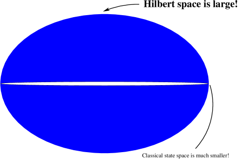
FIG. 12.: Schematic picture of the whole Hilbert space, including entangled states, and the smaller space comprising only the disentangled states expected by a classical physicist.

Going back to our starting point, we say that we are able to hold and manipulate $n$ qubits when we can prepare and keep $n$ beams of light, $n$ two-level atoms or $n$ spin-$\frac{1}{2}$ particles in a joint state $|\psi\rangle$ given by any arbitrary superposition of the $2^{n}$ state vectors which can take the form

$$|\psi\rangle=\sum_{i_{1},\ldots,i_{n}=0}^{1}\alpha_{i_{1}\ldots i_{n}}|i_{1}\ldots i_{n}\rangle$$ (185)

with $2^{n}$ complex amplitudes $\alpha_{i_{1}\ldots i_{n}}$. The actual preparation of such a state presents a tremendous experimental task no matter which constituents subsystems you choose. You need to carefully control and ”engineer” the interaction among all the constituent components to choose the state you want and at the same time you have to protect the joint state against environmental noise. To date, this is possible with only a few qubits and many people are skeptical about radical improvements in the near future. The prospect of implementing quantum computation, that requires manipulation of many qubits to be effective, seems far beyond present capabilities.

C The quantum information content of a quantum system in qubits

We want to make up for the pessimistic tone that ended the last section with the discussion of an interesting feature of quantum information that might be useful in case devices based on quantum information theory are ever built. We will explain how an arbitrary quantum state of a composite system comprised of $n$ interacting 2-level atoms, can be compressed and transmitted by sending a number $m<n$ of qubits. As advertised in chapter 3, this procedure justifies the use of the qubit as the unit of quantum information and by analogy with classical data compression partly justifies the otherwise misleading name $qubit$. We proceed in close mathematical analogy to the classical case studied in section II E and see how well we can compress quantum states, ie. how many qubits are needed to describe a quantum state. We first give a simple example, that illustrates the key ideas, and then we reiterate these ideas in a slightly more general and formal way.

1 Quantum data compression: a simple example

Let us begin with the following very simple example, which is in fact essentially classical, but displays all the relevant ideas of the more general case. Consider a quantum source that emits two-level systems with probability $p_{0}=0.95$ in state $|0\rangle$ and with probability $p_{1}=1-p_{0}=0.05$ in the orthogonal state $|1\rangle$. Our knowledge of this preparation procedure for a single qubit is represented by the density operator ${\hat{\rho}}$ given by

$${\hat{\rho}}=0.95|0\rangle\langle 0|+0.05|1\rangle\langle 1|$$ (186)

Note, that the two states generated by the oven have been chosen to be orthogonal for simplicity. We will consider the more general case later. For the time being, let us consider blocks of $7$ qubits generated by the source described above. Clearly any sequence of qubits in states $|0\rangle$ and $|1\rangle$ is possible, but some are more likely than others. In fact, typically you will find either a sequence that contains only qubits in state $|0\rangle$ or sequences with a single qubit in state $|1\rangle$ and all others in state $|0\rangle$, as shown below:

$$|\psi_{000}\rangle = |0\rangle|0\rangle|0\rangle|0\rangle|0\rangle|0\rangle|0\rangle$$ (187)

$$|\psi_{001}\rangle = |0\rangle|0\rangle|0\rangle|0\rangle|0\rangle|0\rangle|1\rangle$$ (188)

$$|\psi_{010}\rangle = |0\rangle|0\rangle|0\rangle|0\rangle|0\rangle|1\rangle|0\rangle$$ (189)

$$|\psi_{011}\rangle = |0\rangle|0\rangle|0\rangle|0\rangle|1\rangle|0\rangle|0\rangle$$ (190)

$$|\psi_{100}\rangle = |0\rangle|0\rangle|0\rangle|1\rangle|0\rangle|0\rangle|0\rangle$$ (191)

$$|\psi_{101}\rangle = |0\rangle|0\rangle|1\rangle|0\rangle|0\rangle|0\rangle|0\rangle$$ (192)

$$|\psi_{110}\rangle = |0\rangle|1\rangle|0\rangle|0\rangle|0\rangle|0\rangle|0\rangle$$ (193)

$$|\psi_{111}\rangle = |1\rangle|0\rangle|0\rangle|0\rangle|0\rangle|0\rangle|0\rangle\;\;.$$ (194)

The probability that you will get one of the above sequences is $p_{likely}=(0.95)^{7}+7(0.95)^{6}(0.05)=0.955$. Of course, these ’typical’ states can be enumerated using just three binary digits, i.e. $3$ binary digits are sufficient to enumerate $95.5\%$ of all occurring sequences. This procedure is analogous to labeling the typical sequences of 0s and 1s shown in figure 6 except that we now ’enumerate’ the typical sequences with ’quantum states’. Now, let us see how we can use this fact quantum mechanically. We define a unitary transformation that has the following effect:

$$U|0\rangle|0\rangle|0\rangle|0\rangle|0\rangle|0\rangle|0\rangle = |0\rangle|0\rangle|0\rangle|0\rangle|0\rangle|0\rangle|0\rangle$$ (195)

$$U|0\rangle|0\rangle|0\rangle|0\rangle|0\rangle|0\rangle|1\rangle = |0\rangle|0\rangle|0\rangle|0\rangle|0\rangle|0\rangle|1\rangle$$ (196)

$$U|0\rangle|0\rangle|0\rangle|0\rangle|0\rangle|1\rangle|0\rangle = |0\rangle|0\rangle|0\rangle|0\rangle|0\rangle|1\rangle|0\rangle$$ (197)

$$U|0\rangle|0\rangle|0\rangle|0\rangle|1\rangle|0\rangle|0\rangle = |0\rangle|0\rangle|0\rangle|0\rangle|0\rangle|1\rangle|1\rangle$$ (198)

$$U|0\rangle|0\rangle|0\rangle|1\rangle|0\rangle|0\rangle|0\rangle = |0\rangle|0\rangle|0\rangle|0\rangle|1\rangle|0\rangle|0\rangle$$ (199)

$$U|0\rangle|0\rangle|1\rangle|0\rangle|0\rangle|1\rangle|0\rangle = |0\rangle|0\rangle|0\rangle|0\rangle|1\rangle|0\rangle|1\rangle$$ (200)

$$U|0\rangle|1\rangle|0\rangle|0\rangle|0\rangle|1\rangle|0\rangle = |0\rangle|0\rangle|0\rangle|0\rangle|1\rangle|1\rangle|0\rangle$$ (201)

$$U|1\rangle|0\rangle|0\rangle|0\rangle|0\rangle|1\rangle|0\rangle = |0\rangle|0\rangle|0\rangle|0\rangle|1\rangle|1\rangle|1\rangle\;\;.$$ (202)

In this case the unitary transformation is a matrix that maps a set of 8 orthogonal column vectors on another set of 8 orthogonal vectors in a complex vector space of dimension $2^{7}$. The effect of this unitary transformation is to compress the information about the typical sequences into the last three qubits, while the first four qubits are always in the same pure state $|0\rangle$ and therefore do not carry any information. However, when $U$ acts on other, less likely, sequences it will generate states that have some of the first four qubits in state $|1\rangle$. Now comes the crucial step, we throw away the first four qubits and obtain a sequence of three qubits:

$$|0\rangle|0\rangle|0\rangle|0\rangle|0\rangle|0\rangle|0\rangle \rightarrow |0\rangle|0\rangle|0\rangle$$ (203)

$$|0\rangle|0\rangle|0\rangle|0\rangle|0\rangle|0\rangle|1\rangle \rightarrow |0\rangle|0\rangle|1\rangle$$ (204)

$$|0\rangle|0\rangle|0\rangle|0\rangle|0\rangle|1\rangle|0\rangle \rightarrow |0\rangle|1\rangle|0\rangle$$ (205)

$$|0\rangle|0\rangle|0\rangle|0\rangle|0\rangle|1\rangle|1\rangle \rightarrow |0\rangle|1\rangle|1\rangle$$ (206)

$$|0\rangle|0\rangle|0\rangle|0\rangle|1\rangle|0\rangle|0\rangle \rightarrow |1\rangle|0\rangle|0\rangle$$ (207)

$$|0\rangle|0\rangle|0\rangle|0\rangle|1\rangle|0\rangle|1\rangle \rightarrow |1\rangle|0\rangle|1\rangle$$ (208)

$$|0\rangle|0\rangle|0\rangle|0\rangle|1\rangle|1\rangle|0\rangle \rightarrow |1\rangle|1\rangle|0\rangle$$ (209)

$$|0\rangle|0\rangle|0\rangle|0\rangle|1\rangle|1\rangle|1\rangle \rightarrow |1\rangle|1\rangle|1\rangle$$ (210)

Therefore we have compressed the $7$ qubits into $3$ qubits. Of course we need to see whether this compression can be undone again. This is indeed the case, when these three qubits are passed on to some other person, this person then adds four qubits all in the state $|0\rangle$ and then applies the inverse unitary transformation $U^{-1}$ and obtains the states in equation 199 back. This implies that this person will reconstruct the correct quantum state in at least $95.5\%$ of the cases and he has achieved this sending only $3$ qubits. As we showed in the classical case (see equation 13), in the limit of very long blocks composed of $n$ qubits, our friend will be able to reconstruct almost all quantum states by sending only $nH(0.95)=0.2864n$ qubits. Note that this procedure also works when we have a superposition of states. For example, the state

$$|\psi\rangle=\alpha|0\rangle|0\rangle|0\rangle|0\rangle|0\rangle|0\rangle|0\rangle+\beta|0\rangle|0\rangle|0\rangle|0\rangle|0\rangle|0\rangle|1\rangle$$ (211)

can be reconstructed perfectly if we just send the state of three qubits given below:

$$|\psi\rangle=\alpha|0\rangle|0\rangle|0\rangle+\beta|0\rangle|0\rangle|1\rangle$$ (212)

Therefore not only the states in equation 199 are reconstructed perfectly, but also all superpositions of these states.

A very similar procedure would work also when we have a source that emits quantum states $|\psi_{i}\rangle$ with probabilities $p_{i}$, giving rise to an arbitrary density operator $\rho=\sum_{i}p_{i}|\psi_{i}\rangle\langle\psi_{i}|$. Unlike the example in equation 186, the states $|\psi_{i}\rangle$ can be $non-orthogonal$ states of a two level system so the resulting density matrix is $not$ in diagonal form. In this slightly more complicated case, the first step consists in finding the eigenvectors and eigenvalues of $\rho$. As the eigenvectors to different eigenvalues are orthogonal, we are then in the situation of equation 186. We can immediately see that the number of qubits that need to be sent, to ensure that the probability with which we can reconstruct the quantum state correctly is arbitrarily close to unity, is given by $n$ times the Shannon entropy of the eigenvalues of $\rho$ which is in turn equal to the von Neumann entropy $S(\rho)$. Since we can reconstruct the quantum state ${\rho}^{\otimes n}$ of a system composed of $n$ qubits by sending only $nS(\rho)$ qubits, we say that $nS(\rho)$ is the quantum information content of the composite system.

2 Quantum data compression via Landauer’s principle

One may wonder whether the efficiency of quantum data compression can be deduced from Landauers principle and indeed this is possible. Given a source that generates $|\psi_{i}\rangle$ with probabilities $p_{i}$, and gives rise to a density operator $\rho=\sum_{i}p_{i}|\psi_{i}\rangle\langle\psi_{i}|$ we know from section IV B that the entropy of erasure per qubit is given by $S(\rho)kln2$. Now let us assume that we could compress the quantum information in state ${\hat{\rho}}^{\otimes n}$ to $n(S(\hat{\rho})-\epsilon)$ qubits where $\epsilon\geq 0$. The state of each of these qubits will be the maximally mixed state ${\hat{\omega}}=\frac{1}{2}|0\rangle\langle 0|+\frac{1}{2}|1\rangle\langle 1|$ because otherwise we could compress it even further. We can then calculate the entropy of erasure of the $n(S(\rho)-\epsilon)$ qubits in state $\hat{\omega}$ and find of course $n(S(\rho)-\epsilon)S({\hat{\omega}})kln2=n(S(\hat{\rho})-\epsilon)H(\frac{1}{2})kln2=n(S(\hat{\rho})-\epsilon)kln2$. Therefore the total entropy of erasure would be given by the total number of qubits times the entropy of erasure for the qubits $n(S(\hat{\rho})-\epsilon)\times kln2$ which is less than $nS(\hat{\rho})kln2$. This however, cannot be, because Landauer’s principle dictates that the entropy of erasure cannot be less than $S(\rho)kln2$ if the compressed states should hold the same amount of information as the uncompressed states. Therefore, we arrive at a contradiction which demonstrates that the efficiency of quantum data compression is limited by the Von Neumann entropy $S(\rho)$, as classical data compression is limited by the Shannon entropy. This is the answer to the first part of the second searching question in I. We still need to find out whether this similarity between classical and quantum information extends also to the act of copying information.

D Quantum information cannot be copied

In this section, we use Landauer’s erasure principle to argue that unlike classical bits qubits cannot be copied. This result is often termed the no-cloning theorem. The basis of our arguments is a reductio ad absurdum. We show that if Bob can clone an unknown state sent to him by Alice, then he can violate Landauer’s principle. The logical steps of this argument are discussed below in the context of an example.

1. Alice starts by encoding letter $0$ and $1$, occurring with equal probabilities, in the non-orthogonal states $|\psi_{0}\rangle$ and $|\psi_{1}\rangle$

   $$0\longmapsto|\psi_{0}\rangle=|\uparrow\rangle$$ (213)

   $$1\longmapsto|\psi_{1}\rangle=\frac{1}{\sqrt{2}}|\uparrow\rangle+\frac{1}{\sqrt{2}}|\downarrow\rangle.$$ (214)

   We can find the upper bound to the information transmitted per letter by using Landauer’s principle. As discussed in section IV A, the minimum entropy of erasure generated by thermalisation of the carriers’ states is given by $S(\rho)$ where $\rho$ represent the incomplete knowledge that we have of the state of each carrier:

   $$\rho=\frac{1}{2}|\psi_{1}\rangle\langle\psi_{1}|+\frac{1}{2}|\psi_{0}\rangle\langle\psi_{0}|.$$ (215)

   After working out the matrix corresponding to ${\hat{\rho}}$ and plugging it in the formula 161 for the Von Neumann entropy, we find that the entropy of erasure and therefore the information is equal to 0.6008 bits. This is less than 1 bit because the two states are non-orthogonal and the von Neumann entropy is less that the Shannon entropy of the probability distribution with which the states are chosen, i.e. $H(\frac{1}{2})=log2=$1 bit.

2. Alice sends the message states to Bob who has the task to decipher her message. Bob is also informed of how Alice encoded her letters (but of course he does not know the message!) and uses this information in his guess. No matter how clever Bob is, he will never recover more information than what Alice encoded (i.e. more than 0.6008 bits).

3. Now let us assume that Bob owns a machine that can clone an arbitrary unknown quantum state and he uses it to clone an arbitrary number of times each of the message-states Alice sends to him.

4. However, if Bob can clone the state of the message-system, then, upon receiving any of the two states $|\psi_{0}\rangle$ or $|\psi_{1}\rangle$ he can create a copy. Since the probability of receiving each state is $\frac{1}{2}$, Bob will end up holding either two copies of the first $|\psi_{0}\rangle|\psi_{0}\rangle$ or two copies of the second state $|\psi_{1}\rangle|\psi_{1}\rangle$. We can compute the density operator that describes this situation following the rules described in section III:

   $$\rho_{twocopies}=\frac{1}{2}|\psi_{0}\rangle|\psi_{0}\rangle\langle\psi_{0}|\langle\psi_{0}|+\frac{1}{2}|\psi_{1}\rangle|\psi_{1}\rangle\langle\psi_{1}|\langle\psi_{1}|$$ (216)

   The density operator $\rho_{twocopies}$ is represented a $4\times 4$ matrix. After finding the eigenvalues of this matrix we can calculate its Von Neumann entropy $S(\rho_{twocopies})$. This is a measure of the classical information that Bob has about the letter received after cloning. We find:

   $$S(\rho_{twocopies})=0.8113>0.6008\;.$$ (217)

   Therefore the information content of the state has increased and if we would push this further and create infinitely many copies, then Bob would perfectly distinguish between the two non-orthogonal states and he could extract one bit of information per letter-state received. This, however, is not possible as we cannot extract more info than Alice has originally encoded.

The no-cloning theorem represents one of the most striking differences between classical and quantum information. We therefore conclude this section on quantum information by completing our answer to the second question posed in the introduction. Quantum information can be compressed in the sense described in section V C, but it cannot be copied as we routinely do with classical information.

VI Entanglement revisited

In the last section, we have always encountered the concept of entanglement as one of the central theme in quantum information theory. However, we never systematically addressed the question of what physical properties make entangled states peculiar and how they can be engineered and exploited for practical purposes in the lab. We now embark on this task. Our approach here will be based on worked out examples. We have chosen the same approach and numerical examples as in reference [17], so that the reader who masters the topics presented here can easily jump to a more comprehensive and mathematical treatment. Throughout the following sections, we concentrate exclusively on bipartite entanglement for which a sufficient understanding has been reached.

A The ebit

In section III B 5, we saw that any arbitrary superposition of the basis vectors ($|01\rangle$, $|11\rangle$, $|00\rangle$, $|10\rangle$) represents the physical state of a bipartite system. So that must be true also for the vector $|\sigma_{AB}\rangle$ given by:

$$|\sigma_{AB}\rangle=\alpha|01\rangle+\beta|10\rangle.$$ (218)

where $\alpha$ and $\beta$ are two arbitrary $complex$ numbers such that $|\alpha|^{2}+|\beta|^{2}=1$. We quickly remind the reader that, according to the rules of quantum mechanics, $|\alpha|^{2}$ is the probability for finding the first system in $|0\rangle$ and the second in state $|1\rangle$ after a measurement, whereas $|\beta|^{2}$ is the probability of finding the first system in state $|1\rangle$ and the second $|0\rangle$. The states of systems $A$ and $B$ are clearly anti-correlated. But this is not the whole story.

We remind the reader that what is remarkable about $|\sigma_{AB}\rangle$ is that it is impossible to write it as a product state. The state $|\sigma_{AB}\rangle$ is represented by a vector in the enlarged Hilbert space $H_{AB}$ that cannot be factorised as the tensor product of two vectors in $H_{A}$ and $H_{B}$. Therefore, we reach the conclusion that $|\sigma_{AB}\rangle$ does represent the state of a bipartite system, but we cannot assign a definite state to its constituent components. In fact, even the terminology constituent components is a bit misleading in this context. We emphasize that the systems $A$ and $B$ can be arbitrary far from each other but nevertheless constitute a single system. The entanglement of the bipartite state $|\sigma_{AB}\rangle$ is then a measure of the non-local correlations between the measurement outcomes for system A and system B alone. These correlations are the key to the famous Bell inequalities and origin of much philosophical and physical debate [31] and more recently the basis for new technological applications [1, 2, 3, 4, 5, 6, 7, 8, 5, 9, 10, 4]

A basic question that arises in this context is how much entanglement is contained in an arbitrary quantum state? A general answer to this question has not been found yet, although quite a lot of progress has been made [7, 32, 35, 34] . In this article we confine ourselves to the simplest case of bipartite entanglement for which an extensive literature exists. As a first step we define the unit of entanglement for a bipartite system as the amount of entanglement contained in the maximally correlated state:

$$|\sigma_{AB}\rangle=\frac{1}{\sqrt{2}}|10\rangle+\frac{1}{\sqrt{2}}|01\rangle\;.$$ (219)

We call this fundamental unit the ebit in analogy with the qubit and the bit. Note that this state differs from the maximally correlated state $|\psi_{AB}\rangle$ in equation 99, only by a local unitary transformation and should therefore contain the same amount of entanglement. The reason behind the name ebit will be clear after reading section VI D, where we explain how to turn any multipartite entangled systems into a group of $m$ ebits plus some completely disentangled (product) states, just by using local operations and classical communication. There is another reason, related to communication, for choosing state Eq. (219) as the unit of entanglement. One can show that the ebit is the minimal amount of entanglement that allows the non-local transfer of one unit of quantum information. Such a procedure is quantum teleportation of one qubit of quantum information [9, 7]. For our purposes this process can be compared to the working of a hypothetical quantum fax machine (see figure 13).

FIG. 13.: A schematic picture of quantum state teleportation. A qubit in an unknown quantum state is entered into a machine which consumes one unit of entanglement (ebit) and a local measurement whose four possible outcomes are transmitted to the receiver. As a result the original state of the qubit is destroyed at the senders location and appears at the receivers end. The mathematical details can be found in [9, 7]

Alice, who is very far away from Bob can transmit the unknown quantum state of a qubit to Bob by using this device. In what follows, we regard the quantum fax machine as a black box (figure 13). We are not interested in the internal mechanism of this device nor in the procedures that Alice and Bob have to learn to make it work. All we are interested are the resources that this machine exploits and of course the result that it produces. It turns out that the only two resources needed to send the unknown quantum state of ONE qubit from Alice to Bob are:

1. ONE maximally entangled pair of particles shared between Alice and Bob (represented by a wiggled line in figure 13). For example, Bob is holding system B and Alice system A and the joint state is $|\sigma_{AB}\rangle$ in equation 219.

2. TWO classical bits that Alice must send to Bob through a classical channel like an ordinary phone (represented by the telephone line in figure 13).

If these two resources are available Alice and Bob can successfully transmit the unknown quantum state of a qubit. The existence of such quantum fax machines suggests that the sending of 1 qubit can be accomplished by 1 ebit plus 2 classical bits.

There is an important difference between the quantum and classical fax machine. After Alice sends the qubit to Bob the state of her qubit (the original copy of the quantum message) gets destroyed. Only one qubit survives the process and is in Bob’s hands. Incidentally also the ebit that acted as a sort of quantum channel during the communication is destroyed. Those who were thinking of buying a quantum fax machine and use it also as a quantum photocopier will be disappointed. The reason for this is the no cloning theorem [36] discussed in section V D. Furthermore if we could clone we would violate the law of the non-increase of entanglement under local operations [7] that we will explore in the next few sections.

B Classical versus quantum correlations

In the last section we mentioned that bipartite entanglement is a measure of quantum correlations between two spatially separated parts. We now want to make clear what is meant by quantum and classical correlations in the context of an example.

Consider an apparatus that generates two beams of light in the mixed state ${\hat{\rho}_{AB}}$ given by:

$${\hat{\rho}_{AB}}=\frac{1}{2}|HH\rangle\langle HH|+\frac{1}{2}|VV\rangle\langle VV|$$ (220)

The notation above represents our incomplete knowledge of the preparation procedure, namely the fact that we know that the two beams were prepared either both vertically polarized or both horizontally polarized but we do not know which of these two alternatives occurred. If we perform a polarization measurement on these two beams by placing the polarizer along the axis of vertical or horizontal polarization we will find half of the time the two beams both polarized in the vertical direction and half of the time in the horizontal direction. In this sense, the measurement outcomes for the two beams are $maximally$ correlated. We say that mixed states like ${\hat{\rho}_{AB}}$ are classically correlated. The adjective classical is there not because the systems considered are necessarily classical macroscopic objects, but rather because the origin of this correlation can be perfectly explained in terms of classical reasoning. It simply arises from our lack of complete knowledge of the preparation procedure.

If we represent the distinguishable single beam states $|H\rangle$ and $|V\rangle$ as the orthogonal column vectors $\left(\begin{array}[]{c}1\\ 0\end{array}\right)$ and $\left(\begin{array}[]{c}0\\ 1\end{array}\right)$, respectively, we can then write the state ${\hat{\rho}_{AB}}$ in matrix form following the guidance provided in equations 94, 121 and 152

$${\hat{\rho}_{AB}}=\frac{1}{2}\left(\begin{array}[]{c c c c}1&0&0&0\\ 0&0&0&0\\ 0&0&0&0\\ 0&0&0&1\end{array}\right)\;.$$ (221)

We now turn our attention to the maximally entangled state $|\psi_{AB}\rangle=\frac{1}{\sqrt{2}}|HH\rangle+\frac{1}{\sqrt{2}}|VV\rangle$. When the two beams are prepared in this pure state the outcomes of a polarization measurement along the vertical and horizontal directions are maximally correlated as in the previous case. However, there is an important difference between the two. The maximally entangled state is a pure state. That means there is nothing more that we can in principle know about it than what we can deduce from its wave-function. So the origin of this correlation is not lack of knowledge, because for a pure state we have complete information on the preparation procedure. The state $|\psi_{AB}\rangle$ can be represented mathematically using the same conventional choice of basis vectors and following the same hints as the density matrix:

$$|\psi_{AB}\rangle\langle\psi_{AB}|=\frac{1}{2}\left(\begin{array}[]{c c c c}1&0&0&1\\ 0&0&0&0\\ 0&0&0&0\\ 1&0&0&1\end{array}\right)\;\;.$$ (222)

A quick look at the entries of the matrix above shows that ${\hat{\rho}_{AB}}$ is indeed a different mathematical object than $|\psi_{AB}\rangle\langle\psi_{AB}|$. But this mathematical difference on paper means nothing if we cannot interpret it physically. In other words, how can you distinguish in the lab these two states from each other, if they seem to have the same measurement statistics? The answer is: turn the polarizer and measure again! Unfortunately, we cannot perform this crucial experiment in front of the reader but we can try to model it on paper and predict the results on the basis of our knowledge of measurement theory as developed in section III.

For example imagine that you turn the polarizer by $45^{o}$. Now you have two new orthogonal directions that you can label $x$ and $y$. These new directions are analogous to the directions of horizontal and vertical polarization considered before.

The new polarization states can be expressed in terms of the old ones by using simple vector decomposition:

$$|X\rangle=\frac{1}{\sqrt{2}}|V\rangle+\frac{1}{\sqrt{2}}|H\rangle$$ (223)

$$|Y\rangle=\frac{1}{\sqrt{2}}|V\rangle-\frac{1}{\sqrt{2}}|H\rangle$$ (224)

It seems natural to ask the question: are the measurement outcomes of the two beams still maximally correlated (ie. the beams are both found in either state $|X\rangle$ or state $|Y\rangle$? To answer this question, we can check whether there is a non-vanishing probability of finding one of the beams in state $|X\rangle$ and the other in state $|Y\rangle$. To do that we have to first construct the column vectors representing $|X\rangle$ and $|Y\rangle$ (see equation 29), then the single beam projectors $|X\rangle\langle X|$ and $|Y\rangle\langle Y|$ (see equation 52) and finally the joint projector ${\hat{P}}$ given by $|X\rangle\langle X|\otimes|Y\rangle\langle Y|$ (see equation 131). We will not deprive the reader from the pleasure of explicitly constructing the $4\times 4$ matrix representing ${\hat{P}}$, a task well within reach if one follows the hints given above. Once you have ${\hat{P}}$, you can calculate the probabilities of finding the two beams anti-correlated in the new basis (ie. when you measure with the polarizer turned by $\frac{\pi}{2}$) for both the classically and quantum correlated states ($Prob^{\rho}_{anticorrelated}$ and $Prob^{\psi}_{anticorrelated}$). Note that turning the polarizer affects the measurement not the preparation procedure of states ${\hat{\rho}_{AB}}$ and $|\psi_{AB}\rangle\langle\psi_{AB}|$ that must be prepared exactly as before. By using equation 53 we then find:

$$Prob^{\rho}_{anticorrelated}=tr\{{\hat{P}}{\hat{\rho}_{AB}}\}=\frac{1}{4}.$$ (225)

$$Prob^{\psi}_{anticorrelated}=tr\{{\hat{P}}|\psi_{AB}\rangle\langle\psi_{AB}|\}=0.$$ (226)

The results above demonstrate that the the two states in eq. 220 and 222 possess different forms of correlations which we revealed by going from the ’standard’ basis to a rotated basis. This trick is the basis for the formulation of Bell inequalities [31] which show that a combination of correlations measured along different rotated axes cannot overcome a certain value when the state on which they are measured is classically correlated. If we measure the same set of correlations on a quantum mechanically entangled state, then this limit can be exceeded and this has been confirmed in experiments.

C How to create an entangled state?

Another way to gain an intuitive understanding of the differences between quantum and classical correlations is to investigate the preparation procedures of states $|\psi_{AB}\rangle$ and ${\hat{\rho}_{AB}}$. The latter can be generated by two distant parties, Alice and Bob, who have a beam of light each and are allowed only 1) local operations on their own beam and 2) classical communication via an ordinary phone. The entangled state instead cannot be created unless Bob and Alice let their beams interact. More explicitly, suppose that Alice and Bob are $both$ given each one beam of light and are asked to create first the mixed state ${\hat{\rho}_{AB}}$ and then the pure entangled state $|\psi_{AB}\rangle$. What operations are they going to do, if they start with the same resources in the two cases?

Let’s first consider ${\hat{\rho}_{AB}}$. Alice who is in London phones Bob who is in Boston and tells him to prepare his beam horizontally polarized. That amounts to sending one bit of classical information (ie. either H or V). Then she prepares her beam also horizontally polarized. After completing this operation the two have constructed the product state $|HH\rangle$. Now they repeat the same procedure many time and each time they store their beams in two rooms (one in London and the other in Boston) clearly labeled with the $SAME$ number (for example, ”experiment 1”) and with an H to indicate that the beam is horizontally polarized. After doing this for $n$ times, they perform an analogous procedure to create $|VV\rangle$ and they fill other $n$ rooms carefully labeled with the same system, but they write V rather than H, to indicate that they store vertically polarized beams. Now, the two decide to erase the letter H or V from each room but they keep the labeling number. After the erasure, Alice and Bob have an incomplete knowledge of the state of the two beams contained in each pair of room labeled with the same number. They know that the two beams are either in state $|HH\rangle$ or $|VV\rangle$ but they do not know which. The information the two hold on each of the pair of correlated beams contained in rooms labeled with the same number is correctly described by ${\hat{\rho}_{AB}}$. They have in fact created an ensemble of pair of beams in state ${\hat{\rho}_{AB}}$ by acting locally and just using phone calls. The example above is a bit of a ”theorist’s description of what is going on in the lab”. The example captures the crucial fact that classical correlations arise from 1) local manipulations of the quantum states and 2) erasure of information that in principle is available to some more $knowledgeable$ observers.

The situation is very different when Alice and Bob want to create an entangled state and they start with two completely disentangled product states like one beam in Boston and another independent one in London. In this situation, one of the two has to take the plane and bring his or her beam to interact with the other. Only at that point can entanglement be created. In fact, one of the basic results of quantum information theory is that the net amount of entanglement in a system cannot be increased by using classical communication and local operations only. So, if Alice and Bob start with no entanglement at all, then they are forced to bring the two beams together and let them interact in order to create entanglement. We now would like to illustrate an example of two beams that are initially in a disentangled state and become entangled by interacting with each other. Suppose that Alice and Bob hold a beam each polarized at an angle $\frac{\pi}{4}$ (see equation 223) . The two beams are initially far away from each other so they are not interacting. The joint system can be described mathematically by the product state $|\psi_{AB}(0)\rangle$ given below:

$$|\psi_{AB}(0)\rangle = (\frac{1}{\sqrt{2}}|H\rangle_{A}+\frac{1}{\sqrt{2}}|V\rangle_{A})\otimes(\frac{1}{\sqrt{2}}|H\rangle_{B}+\frac{1}{\sqrt{2}}|V\rangle_{B})\;\;.$$ (227)

$$= \frac{1}{2}\left(\begin{array}[]{c}1\\ 1\end{array}\right)\otimes\left(\begin{array}[]{c}1\\ 1\end{array}\right)\;\;.$$ (232)

$$= \frac{1}{2}\left(\begin{array}[]{c}1\\ 1\\ 1\\ 1\end{array}\right)\;\;.$$ (237)

The two beams in the product state $|\psi_{AB}(0)\rangle$ are brought together and they start interacting with each other. The time evolution of the original state is determined by the joint Hamiltonian of the system ${\hat{H}}$ that is represented mathematically by a $4\times 4$ hermitian matrix because it has to operate on vectors in the enlarged Hilbert space. Let us pick up an Hamiltonian of this type, something easy so the calculation does not get too complicated and let us see what happens.

$${\hat{H}}=\left(\begin{array}[]{c c c c}1&0&0&0\\ 0&1&0&0\\ 0&0&1&0\\ 0&0&0&-1\end{array}\right)\;\;.$$ (238)

The basis vectors used to write the Hamiltonian ${\hat{H}}$ are the same used to write $|\psi_{AB}(0)\rangle$ in equation 237. Since the matrix in equation 238 is diagonal, we can read out the eigenstates and eigenvalues of the Hamiltonian. They are the state vectors $|HH\rangle$, $|HV\rangle$, $|VH\rangle$ and $|VV\rangle$ and the corresponding eigenvalues are equal to $1$, $1$, $1$ and $-1$.

We can now write down the time evolution of the state $|\psi_{AB}(0)\rangle$ by solving the Schrödinger equation with the Hamiltonian ${\hat{H}}$:

$$i\hbar\frac{\partial\psi_{AB}(t)}{\partial t}={\hat{H}}\psi_{AB}(t)$$ (239)

The Schrödinger equation above is really a set of four linear differential equations one for each component of the four dimensional vector representing $\psi_{AB}(t)$. Usually, these four differential equations would be coupled by the Hamiltonian so you would have to diagonalize the corresponding matrix. In this case however the Hamiltonian is already diagonal so we can redily write the solution of this set of equations in vector form as:

$$\psi_{AB}(t)=\exp(\frac{-i}{\hbar}{\hat{H}}t)\psi_{AB}(0).$$ (240)

The exponential of the Hamiltonian $\exp(\frac{-i}{\hbar}{\hat{H}}t)$ is the diagonal matrix whose eigenvalues are the exponential of the eigenvalues of the Hamiltonian’s matrix (see equation 161 and discussion below). The reader can also check that this time evolution matrix is unitary. After time $t=\frac{\pi\hbar}{2}$ (never mind the units) the matrix can be written as:

$$\exp(\frac{-i}{\hbar}{\hat{H}}t) = \left(\begin{array}[]{c c c c}e^{\frac{-i\pi}{2}}&0&0&0\\ 0&e^{\frac{-i\pi}{2}}&0&0\\ 0&0&e^{\frac{-i\pi}{2}}&0\\ 0&0&0&e^{\frac{+i\pi}{2}}\end{array}\right)\;\;.$$ (245)

$$= \left(\begin{array}[]{c c c c}-i&0&0&0\\ 0&-i&0&0\\ 0&0&-i&0\\ 0&0&0&i\end{array}\right)\;\;.$$ (250)

According to equation 240, you can now write down the vector $\psi_{AB}(t)$ just by multiplying the unitary matrix in equation 250 times the column vector $\psi_{AB}(0)$ given in equation 237. The result is that after time $\frac{\pi\hbar}{2}$ the state vector representing the system is:

$$|\psi_{AB}(t)\rangle=\frac{-i}{2}\left(\begin{array}[]{c}1\\ 1\\ 1\\ -1\end{array}\right).$$ (251)

You can check by inspection that the state in equation 251 is entangled (ie. it cannot be factorized). The more ambitious reader may consult reference [17] that explains in simple terms the systematic criteria to check whether the state of a bipartite system is entangled or not in the context of this example.

Whatever way you choose to convince yourself that the state above is entangled the conclusion is the same. States that can be factorized arise mathematically only for very special choices of the entries of the corresponding vectors. Under Hamiltonian evolution the value of these entries will change and in general it will not be possible to factorize the state any more. The discussion above shows that the process by which two independent systems in a product state like $|\psi_{AB}(0)\rangle$ get entangled is indeed quite natural provided that the two systems are brought together and left to interact with each other. However, most interaction will not lead to a maximally entangled state. It is therefore important for applications like teleportation to devise techniques by which one can distill a set of ebits from an ensemble of partially entangled states like $|\psi_{AB}(t)\rangle$ in equation 251. This is the subject of the next section.

D Entanglement distillation

We emphasize that the fundamental law of quantum information processing does not rule out the possibility to $occasionally$ increase the net amount of entanglement in a system by using local operations and classical communication only, provided that $on$ $average$ the net amount of entanglement is not increased. This implies that it should be possible to devise strategies to turn a partially entangled pair of particles into an ebit provided that this strategy sometimes leads to an increase and other times to a loss of entanglement so that on average the ”entanglement balance” stays the same. We first consider a simple example of entanglement distillation and then we look at the efficiency of a general distillation procedure by using Landauer’s principle.

1 A simple example

Alice is still in London and Bob in Boston. They share a non maximally entangled pair of particles in the state $|\psi_{AB}\rangle=\alpha|00\rangle+\beta|11\rangle$, where $\alpha$ $\neq$ $\beta$. They want to turn it into an ebit but they are only allowed to act locally on their own particle but not to let the two interact. Furthermore, their communication must be limited to classical bits sent over an ordinary channel, nothing fancy like sending or teleporting quantum states is allowed. The reason why we demand such tough conditions on Bob and Alice and we insist on them not to freely meet up is because we want to investigate the issue of locality versus non-locality. This is really the main theme behind our study of entanglement, so we have to be extra careful in keeping track of what they do. That still leaves a lot of room for manipulation on both Alice’s and Bob’s side. For example the two can add other particles on their own side and let them interact with the entangled particle they are holding and perform measurements on them. We now describe what operations the two perform in order to distill one ebit.

1. Alice adds another particle in state $|0_{A}\rangle$ on her side. Note that the subscript $A$ denotes particles on Alice’s side and $B$ on Bob’s side. Now the joint state of the entangled pair plus the extra particle is given by the product state $|\psi_{tot}\rangle$ given below:

   $$|\psi_{tot}\rangle=|0_{A}\rangle\otimes(\alpha|0_{A}\rangle|0_{B}\rangle+\beta|1_{A}\rangle|1_{B}\rangle).$$ (252)

   We can collect the states of the two particles on Alice side in the same four dimensional column vector and rewrite equation 252 as:

   $$|\psi_{tot}\rangle=\alpha|00\rangle_{A}|0_{B}\rangle+\beta|01\rangle_{A}|1_{B}\rangle$$ (253)

2. Now Alice performs a unitary transformation ${\hat{U}}$ on her two particles. As we mentioned in the previous section, a unitary transformation can be implemented by letting the joint system evolve for a certain time as dictated by a suitably chosen Hamiltonian (see example in equation 250). The unitary transformation ${\hat{U}}$ that Alice needs to implement on the joint state of her two particles is given below in matrix form:

   $${\hat{U}}=\left(\begin{array}[]{c c c c}\frac{\beta}{\alpha}&0&-\frac{\sqrt{\alpha^{2}-\beta^{2}}}{\alpha}&0\\ 0&1&0&0\\ \frac{\sqrt{\alpha^{2}-\beta^{2}}}{\alpha}&0&\frac{\beta}{\alpha}&0\\ 0&0&0&1\end{array}\right)\;\;.$$ (254)

   The reader can check that, when the unitary transformation is applied on her states $|00\rangle_{A}$ and $|01\rangle_{A}$, Alice achieves the following:

   $${\hat{U}}|00\rangle_{A} = \frac{\beta}{\alpha}|00\rangle_{A}+\frac{\sqrt{\alpha^{2}-\beta^{2}}}{\alpha}|10\rangle_{A}\;\;;$$ (255)

   $${\hat{U}}|01\rangle_{A} = |01\rangle_{A}\;\;.$$ (256)

   Hence, when the unitary transformation ${\hat{U}}$ is applied to the joint state of the three particles $|\psi_{tot}\rangle$, the state of the particle on Bob’s side is unaffected whereas the state of the two on Alice’s side is changed according to equation 256:

   $${\hat{U}}|\psi_{tot}\rangle = \beta|00\rangle_{A}|0_{B}\rangle$$ (258)

   $$+\sqrt{\alpha^{2}-\beta^{2}}|10\rangle_{A}|0_{B}\rangle+\beta|01\rangle_{A}|1_{B}\rangle.$$

   We can split Alice’s vector states in equation 258 and isolate the state of the entangled pair from the state of the particle added on Alice’s side by writing the latter first in the equation below:

   $${\hat{U}}|\psi_{tot}\rangle=\sqrt{2}\beta|0_{A}\rangle\frac{|0_{A}\rangle|0_{B}\rangle+|1_{A}\rangle|1_{B}\rangle}{\sqrt{2}}$$ (259)

   $$+\sqrt{\alpha^{2}-\beta^{2}}|1_{A}\rangle|0_{A}\rangle|0_{B}\rangle\;\;.$$ (260)

3. Now, Alice decides to perform a measurement on the extra particle she is holding on her side. She chooses the observable that has $|0\rangle$ and $|1\rangle$ as its eigenstates. There are two possible scenarios:

   a) Alice finds the extra particle in state $|0\rangle$. Then the total state is $|0\rangle_{A}\otimes\frac{1}{\sqrt{2}}(|0_{A}0_{B}\rangle+|1_{A}1_{B}\rangle)$. Alice and Bob share a maximally entangled state. This event occurs with probability $2\beta^{2}$.

   b) Alice finds the extra particle in state $|1\rangle$. Then the total state is $|1_{A}\rangle\otimes|0_{A}0_{B}\rangle$. The procedure was unsuccessful and the two lost their initial entanglement. This possibility occurs with probability $1-2\beta^{2}$.

4. Alice phones Bob and informs him of the measurement outcomes. If the procedure is successful Bob holds his particle otherwise they try again.

A question that arises naturally in this context is the following: what is the maximum number of ebits that Alice and Bob can extract from a large ensemble of $N$ non maximally entangled states? We will answer this question by using Landauer’s erasure principle.

2 Efficiency of entanglement distillation from Landauer’s principle

We start by considering an example of a process that will cause two systems to become entangled: a quantum measurement. A quantum measurement is a process by which the apparatus and the system interact with each other so that correlations are created between the states of the two. These correlations are a measure of the information that an observer acquires on the state of the system if he knows the state of the apparatus.

Consider an ensemble of systems $S$ on which we want to perform measurements using apparatus $A$. A general way to write the state of $S$ is

$$\left|\psi_{S}\right\rangle=\frac{1}{\sqrt{N}}\sum_{i=1}^{N}\left|s_{i}\right\rangle,$$ (261)

where $\left\{\left|s_{i}\right\rangle\right\}$ is an orthogonal basis. In our previous example, the orthogonal basis was given by the vertically and horizontally polarized states. When the apparatus is brought into contact with the system the joint state of $S$ and $A$ is given by

$$\left|\psi_{S+A}\right\rangle=\frac{1}{\sqrt{N}}\sum_{i=1}^{N}\left|s_{i}\right\rangle\left|a_{i}\right\rangle.$$ (262)

The result of the act of measurement is to create correlations (ie. entanglement) between the apparatus and the system. The equation above is a generalization of equation 219.

An observation is said to be imperfect when it is unable to distinguish between two different outcomes of a measurement. Let $A$ be an imperfect measuring apparatus so that $\left\{\left|a_{i}\right\rangle\right\}$ is NOT an orthogonal set. A consequence of the non-orthogonality of the states $|a_{i}\rangle$ is that we are unable to distinguish with certainty the correlated states $|s_{i}\rangle$. There is no maximal correlation between the state of the system and the apparatus, which means that $S$ and $A$ are not maximally entangled). However, suppose that by acting locally on the apparatus we can transform the whole state $\left|\psi_{S+A}\right\rangle$ into the maximally entangled state $|\phi_{S+A}\rangle$:

$$\left|\phi_{S+A}\right\rangle=\frac{1}{\sqrt{N}}\sum_{i=1}^{N}\left|s_{i}\right\rangle\left|b_{i}\right\rangle,$$ (263)

where $\left\{\left|b_{i}\right\rangle\right\}$ IS an orthogonal set. This does not increase the information between the apparatus and the system since we are not interacting with the system at all. In order to assess the efficiency of this distillation procedure we need to find the probability with which we can distill successfully.

The state of the apparatus only, after the correlations are created, is given by the reduced density operator first encountered in section III C 3:

$$tr_{S}(\left|\psi_{S+A}\right\rangle\left\langle\psi_{S+A}\right|)=\rho_{A}.$$ (264)

Landauer’s principle states that to erase the information contained in the apparatus we need to generate in the environment an entropy of erasure larger than $S(\rho_{A})$ and this has to be greater than or equal to the information gain. After we purify the state to $\left|\phi_{S+A}\right\rangle$ with a probability $p$ , we gain $p\log N$ bits of information about the system. In fact, since we have maximal correlations now, the result of a measurement enables us to distinguish between N equally likely outputs. The rest of the state contains no information because it is completely disentangled and therefore there are no correlations between the states of the system and the apparatus. After reading the state of the apparatus we will not gain any useful knowledge on the state of the system.

By Landauer’s principle, the entropy of erasure is greater than or equal to the information gain before purification and this is in turn greater than or equal to the information the observer has after purification, because the apparatus is not interacting with the system so the information can not increase. We thus write

$$S(\rho_{A})\geq p\log N.$$ (265)

The upper bound to purification efficiency is therefore

$$p\leq S(\rho_{A})/\log N.$$ (266)

This bound obtained from Landauer’s principle is actually achievable as has been proven in [32] by construction of an explicit procedure that achieves it. It is nevertheless satisfying that Landauer’s principle is able to give a sharp upper bound with a minimal amount of technicalities and by doing so it provides an informal argument for using the Von Neumann entropy as a measure of bipartite entanglement. With this result we answer the last of the three questions posed in the introduction that have served as guidelines for our exploration of the physical theory of information.

VII Conclusion

This is really the end of our long investigation on the properties of entanglement, classical and quantum information. We hope to have reasonably delivered what we promised in the introduction. Throughout the paper, we used the pedagogical technique of going backwards and forward among different aspects of the subject, each time increasing the level of sophistication of the ideas and mathematical tools employed. This method has the advantage of allowing enough time for ”different layers of knowledge to sediment in the mind of the reader”. Unfortunately, there is also the inevitable side effect that a proper understanding of the subject matter will only follow when the reader goes through the material more than once. For example, the understanding of the differences between quantum and classical information crucially relies on the appreciation of the concepts of classical and quantum correlations that were explicitly studied only at the end of the article. No matter how hard we tried to argue with words previously, a proper grasp of these topics came only after employing more advanced mathematical tools developed in later parts of the paper.

To prevent the reader from feeling lost, we will now attempt to recap the content of the paper. In the first part, the scene was dominated by the Shannon entropy that helped us to define and evaluate the amount of classical information encoded in a classical object or message. We were also able to find a bound on the classical information capacity of a noisy classical channel by using Landauer’s principle. The answer depended once again on the Shannon entropy. Following a brief recap of quantum mechanics, our interest slightly shifted to quantifying the amount of classical information encoded in quantum systems. This was achieved by introducing the Von Neumann entropy. After developing a suitable thermalization procedures to erase information from quantum systems, we managed to employ Landauer’s principle to justify the Holevo bound. This bound expresses the classical information capacity of a noisy quantum channel in terms of the Von Neumann entropy. That completed our investigation of classical information.

We then turned our attention to quantifying the amount of quantum information encoded in a quantum object or message. This result, which is based on quantum data compression, was obtained employing Landauer’s principle and provided a solid basis for the introduction of the qubit as the fundamental unit of quantum information. The answer to this question was once again given by the von Neumann entropy. Quantum information can be compressed, but unlike classical information, it cannot be copied. This was our conclusion after studying the no-cloning theorem with the help of Landauer’s erasure principle.

Motivated by these successes we tried to shed light on the phenomena of entanglement using Landauer’s principle. We explained that creating a pair of entangled states is not difficult after all. Any two systems initially uncorrelated will get entangled just by interacting with each other. However, it is not equally easy to create quantum states that are $maximally$ entangled over large distance. This problem can be overcome by designing suitable distillation procedures by which maximally entangled states, ebits, are produced from an ensemble of non-maximally entangled states without increasing the total amount of entanglement. To some extent this procedure provides a way to measure the amount of entanglement (in ebits) contained in a system composed of only two parts. The efficiency of a distillation procedure was once again expressed in terms of the von Neumann entropy after carrying out a simple analysis based on Landauer’s principle. The von Neumann entropy in quantum information theory is so widespread to justify the claim that the whole field is really about its use and interpretation , as classical information theory was based on the Shannon entropy. [15].

After reading this summary you might have noticed two glaring omissions in our treatment. Firstly, we spent a lot of time discussing the classical information capacity of a noisy classical and quantum channel, but we never mentioned the more interesting problem of the quantum information capacity of a noisy quantum channel. In other words how many qubits can you send through a noisy channel when the letters of your message are encoded in arbitrary quantum states? Secondly, we never mentioned how to generalize our discussion of entanglement measure to the useful and interesting case of entangled states composed of more than two particles.

We reassure the reader that these omissions are not motivated by our compelling desire to meet the deadline for submission of this paper, but rather by the fact that nobody really knows the answer to these fundamental and natural questions. We do not know whether one can push Landauer’s principle to investigate these problems. Landauer’ principle is somehow limited to the erasure of classical information whereas the questions above are completely quantum. However, Landauer’ principle can be used to yield upper bounds to entanglement distillation a completely non-classical procedure. Therefore the hope that Landauer’s principle can shed some light on these unsolved problems may not remain unfulfilled.

Anyway, these final remarks prove the point that, although a large amount of work has been published since Shannon, there is still room for further research in the foundations of information theory. It is also evident that this research belongs to fundamental physics as much as it does to engineering. If you found some of the ideas in this paper fascinating and you wish to start working in the field, you may want to start by studying some further introductory texts such as [15, 16, 17, 19, 20]. Perhaps someday, we will find out the answer to the questions above from you.

Acknowledgments. We would like to thank Miles Blencowe, John Calsamiglia, Susana Huelga, William Irvine, Daniel Jonathan, Peter Knight, Polykarpos Papadopoulos, Stephen Parker, Vlatko Vedral and Shashank Virmani for discussion on the topics involved in this article. This work was supported by EPSRC, the Leverhulme Trust, the EQUIP project of the European Union and the European Science Foundation programme on quantum information theory. The final stages of this work have been carried out at the Erwin Schrödinger Institute in Vienna.

Biographies

Martin Plenio studied in Göttingen (Germany) where he obtained both his Diploma (1992) and his PhD (1994) in Theoretical Physics. After his PhD he joined the Theoretical Quantum Optics group at Imperial College with a Feodor-Lynen grant of the Alexander von Humboldt Foundation as a postdoc. Since January 1998 he is a Lecturer in the Optics Section of Imperial College. His main research interests lie in Quantum Information Theory and Quantum Optics.

Vincenzo Vitelli received his first degree in theoretical physics (2000) from Imperial College. He is now a first year graduate student at Harvard University. His main research interests lie in the area of quantum information theory and statistical physics.

REFERENCES

- [1] A. Ekert and R. Jozsa, Rev. Mod. Phys. 68, 733 (1996).
- [2] V. Vedral and M.B. Plenio, Prog. Quant. Electron. 22, 1 (1998).
- [3] A. Steane, Rep. Prog. Phys. 61, 117 (1998).
- [4] R.J. Hughes, D.M. Alde, P. Dyer, G.G. Luther, G.L. Morgan, M. Schauer, Cont. Phys. 36, 149 (1995).
- [5] Physics World March 1998, Special Issue on Quantum Information: New forms of computation and communication.
- [6] The Physics of Quantum Information, edited by D. Bouwmeester, A.K. Ekert and A. Zeilinger, Springer Verlag, Berlin 2000.
- [7] M.B. Plenio and V. Vedral, Cont. Phys. 39, 431 (1998).
- [8] P.W. Shor, SIAM Rev 41, 303 (1999).
- [9] C.H. Bennett, G. Brassard, C. Crepeau, R. Jozsa, A. Peres, W.K. Wootters, Physical Review Letters 70, 1895 (1993).
- [10] C.H. Bennett and G. Brassard, IEEE Int. C. Comp. , 175 (1984).
- [11] A. Ekert, Phys. Rev. Lett. 67, 661 (1991).
- [12] R. Landauer, IBM Jl. Res. Develop. 5, 183 (1961).
- [13] Maxwell’s Demon: Entropy, Information, Computing, edited by H.S. Leff and A.F. Rex, Adam Hilger (1990)
- [14] C.H. Bennett, Int. J. Theor. Phys. 21, 905 (1982).
-
[15]
J. Preskill, Unpublished lecture notes on
quantum computation,
http://www.theory.caltech.edu/people/preskill/ph229/ -
[16]
M.B. Plenio, Unpublished lectures notes on quantum
mechanics,
http://www.lsr.ph.ic.ac.uk/ plenio/lecture.html -
[17]
H. Mabuchi, Unpublished lectures notes on quantum
mechanics,
http://www.its.caltech.edu/ hmabuchi/Ph98.html - [18] Feynman lectures on computation, edited by A.J.G. Hey and R.W. Allen, Addison-Wesley 1996.
- [19] A. Peres, Quantum Theory: Concepts and Methods, Kluwer Academic Press 1995.
- [20] M. Nielsen and I. Chuang, Quantum Compuation & and Information, Cambridge University Press 2000.
- [21] T.M. Cover and J.A. Thomas, Elements of Information Theory, John Wiley & Sons, Inc., 1991.
- [22] B. Schumacher, lanl e-print quant-ph/0004045.
- [23] L. Szilard, Z. Phys. 53, 840 (1929).
- [24] W.H. Zurek, Phys. Rev A 40, 4731 (1989).
- [25] C. Fuchs and A. Peres, Physics Today March 2000.
- [26] B. Schumacher, Phys. Rev A 51, 2738 (1995).
- [27] M.O. Scully and S. Zubairy, Quantum Optics, Cambridge University Press 1997.
- [28] P. Benioff, Phys. Rev. Lett. 48, 1581 (1982).
- [29] R.P. Feynman, Int. J. Theor. Physics 21, 467 (1982).
- [30] D. Deutsch, Proc. Roy. Soc. A 400, 97 (1985).
- [31] L. Hardy, Contemp. Phys. 39, 419 (1998); P.G. Kwiat and L. Hardy, Am. J. Phys. 68, 33 (2000).
- [32] C.H. Bennett, H. Bernstein, S. Popescu and B. Schumacher, Phys. Rev. A 53, 2046 (1996).
- [33] H.-K. Lo and S. Popescu, quant-ph/9707038; M.A. Nielsen, Phys. Rev. Lett. 83, 436 (1999), G. Vidal, Phys. Rev. Lett. 83, 1046 (1999); D. Jonathan and M.B. Plenio, Phys. Rev. Lett. 83, 1455 (1999); L. Hardy, Phys. Rev. A 60, 1912 (1999).
- [34] V. Vedral and M.B. Plenio, Phys. Rev. A 57, 1619 (1998); M.B. Plenio, S. Virmani and P. Papadopoulos, J. Phys. A 33, L193 (2000); V. Vedral, M.B. Plenio, M. Rippin and P.L. Knight, Phys. Rev. Lett. 78, 2275 (1997); V. Vedral, M.B. Plenio, K. Jacobs and P.L. Knight, Phys. Rev. A 56, 4452 (1997).
- [35] C.H. Bennett, D. DiVincenzo, J.A. Smolin and W.K. Wootters, Phys. Rev. A 53, 3824 (1996); W.K. Wootters, Phys. Rev. Lett. 80, 2245 (1998).
- [36] W.H. Zurek and W.K. Wootters, Nature 299, 802 (1981).
- [37] M.B. Plenio, Phys. Lett. A 263, 281 (1999)
- [38] E. Lubkin, Int. J. Theor. Phys. 26, 523 (1987).
- [39] A.S. Holevo, IEEE Trans. Inf. Theory 44, 269 (1998).
- [40] V. Vedral, Proc. Roy. Soc. A 456, 969 (2000).
- [41] S. Popescu and D. Rohrlich, Phys. Rev. A , (1997)
- [42] N. Gisin, Phys. Lett. A 210, 151 (1996).