Quantum Data Hiding

Abstract

We expand on our work on Quantum Data Hiding [1] – hiding classical data among parties who are restricted to performing only local quantum operations and classical communication (LOCC). We review our scheme that hides one bit between two parties using Bell states, and we derive upper and lower bounds on the secrecy of the hiding scheme. We provide an explicit bound showing that multiple bits can be hidden bitwise with our scheme. We give a preparation of the hiding states as an efficient quantum computation that uses at most one ebit of entanglement. A candidate data hiding scheme that does not use entanglement is presented. We show how our scheme for quantum data hiding can be used in a conditionally secure quantum bit commitment scheme.

I Introduction

It is well known that composite quantum systems can exhibit a variety of nonlocal properties. When two systems are entangled, as when two spins are described by the singlet state $\frac{1}{\sqrt{2}}(|01\rangle-|10\rangle)$, local measurements on the two particles separately can exhibit statistics unexplainable by local hidden variable theories, such as a violation of Bell’s inequalities [2]. An information-theoretic or computational expression of this feature is that entangled states can function as nontrivial resources in quantum communication protocols [3], for example reducing the amount of classical communication needed to perform certain distributed computations.

It has been found that even states without quantum entanglement can exhibit properties of nonlocality that are not present in purely classical systems. The first explorations in this direction were carried out by Peres and Wootters [4], who studied the measurements that could optimally distinguish three nonorthogonal quantum states of which two parties, Alice and Bob, both possess a single copy. They found that any measurement that can be performed using a sequence of local operations supplemented by classical communication between the parties (denoted as LOCC) is not able to retrieve as much information as a global measurement carried out on the joint system. Thus, even though no entanglement is present in this system, the states exhibit nonlocality with respect to their distinguishability. In Ref. [5], where the term ‘quantum nonlocality without entanglement’ was coined, a similar phenomenon was exhibited: it is impossible to use LOCC to perfectly distinguish nine orthogonal bipartite product states, which are perfectly distinguishable when nonlocal actions are allowed.

The results that we have presented in Ref. [1], and on which we expand in the present paper, can be viewed as the strongest possible separation between the power of LOCC versus global operations for the task of distinguishing quantum states. We use the nonlocality of our quantum states to establish a protocol of quantum data hiding: a piece of classical data is hidden from two parties, who each share a part of the data and are allowed to communicate classically. Such a scheme is nontrivial in several respects. First, it is impossible in a purely classical world. Second, it is impossible if the state shared by the two parties is a pure quantum state. This observation follows from the result by Walgate et al. [6] which shows that any two orthogonal bipartite pure quantum states can be perfectly distinguished by LOCC. Third, the scheme is extremely secure; it is possible to make the amount of information obtainable by the parties arbitrarily small; the number of qubits needed is only logarithmic in the information bound.

The quantum data hiding scheme is secure if the parties Alice and Bob cannot communicate quantum states and do not share prior quantum entanglement. In what kind of situations can these conditions be met, and is our scheme of interest? One can imagine a situation in which a third party (the boss) has a piece of data on which she would like Alice and Bob (some employees) to act by LOCC without the sensitive data being revealed to them. We have to assume that the boss controls (1) the channel which connects the two parties and (2) the labs in which the employees operate, so that the boss can use dephasing to prevent the quantum communication and to sweep those labs clean of any entanglement prior to operation. Our scheme is such that at some later stage, the boss can provide the employees with entanglement to enable them to determine the secret with certainty. This feature is used for a conditionally secure bit commitment scheme.

An additional advantage of our scheme, besides its information-theoretic security, is that it can be implemented efficiently; the number of computation steps required, both classical and quantum, grows no faster than a polynomial of the input size. We find an efficient algorithm to prepare the data hiding states which also minimizes the use of quantum entanglement. The algorithm hinges on a surprising connection between an operation known as the Full Twirl [7] and a Twirl over the Clifford group [8]. The Full Twirl is an important operation in the study of entanglement while the Clifford group is an important discrete group in the theory of quantum error correction.

An original goal in our investigations was to establish a data hiding scheme in which a bit could be hidden from LOCC observers, and the data hiding states are unentangled; this would have formed an extremely strong example of ‘nonlocality without entanglement’. Separable (unentangled) hiding states are interesting also because the security for hiding a single bit implies directly that hiding independently distributed multiple bits is also secure. The quantum data hiding protocol using Bell states does not entirely achieve this goal, since it still requires a small amount of entanglement. We propose an alternative quantum data hiding scheme that uses unentangled hiding states. We can only rigorously analyze this scheme for small systems, but on the basis of this analysis, we conjecture this scheme is secure, in the same way as the scheme using Bell states.

Our paper is organized in the following way. In Section II we review the general setup that is needed to analyze the problem of distinguishing a pair of states by LOCC. We derive a condition for any LOCC measurement that attempts to distinguish a pair of states. A related condition has also been discussed in Ref. [9]. In Sections III-V we discuss various aspects of the security of our quantum data hiding protocol: In Section III we discuss the scheme for hiding a single bit. This scheme was first presented and proved secure in Ref. [1]. Our analysis here goes into more detail. Furthermore, in Section III-C we show that the bound on the retrievable information is fairly tight – we find a simple LOCC measurement that retrieves an amount of information close to our proved bound. In Section IV, we digress to show a general result, on how well a single bit can be hidden in two arbitrary orthogonal bipartite states. We obtain a lower bound on the retrievable information, which shows in another way that our scheme has nearly optimal hiding capability. In Section V we extend our protocol to hide $k>1$ bits. We are able to prove a good upper bound on the information retrievable by LOCC, exploiting the symmetry of our hiding states.

In Sections VI-IX, we present various schemes and discussions related to our quantum data hiding protocol: In Section VI we present an efficient algorithm to prepare the data hiding states which also minimizes the use of quantum entanglement. We also prove the equivalence of the Full Twirl and the Twirl over the Clifford group. In Section VII, we discuss the reason that the security for hiding a single bit implies the security for hiding independently distributed multiple bits, and we describe an alternative scheme for hiding bits that uses unentangled hiding states. In Section VIII, we apply the quantum data hiding scheme to construct a conditionally secure quantum bit commitment protocol. We conclude our paper with some discussion and open questions in Section IX.

The discussion up to Section III-B is a prerequisite for all other Sections, which can then be read independently. Throughout the paper, the tensor product of two $d$-dimensional Hilbert spaces is denoted as ${\cal H}_{d}\otimes{\cal H}_{d}$, and a positive semidefinite matrix or operator $A$ (with nonnegative eigenvalues) is denoted as $A\geq 0$.

II General formalism for operations to learn the secret

In quantum mechanics, a large class of state changes can be described using the formalism of quantum operations. A quantum operation is a completely positive map [10, 11] on operators in a Hilbert space $\cal H$. A convenient representation of a quantum operation is the operator-sum representation [12, 10]:

$${\cal S}[\rho]=\sum_{k}S_{k}\rho S_{k}^{\dagger}\,,$$ (1)

where $S_{k}$ are operators acting on $\cal H$. We restrict our discussion to trace preserving quantum operations, for which $\sum_{k}S_{k}^{\dagger}S_{k}=I$. The adjoint of the quantum operation $\cal S$ is ${\cal S}^{\dagger}$, whose action can be expressed as ${\cal S}^{\dagger}[\rho]=\sum_{k}S_{k}^{\dagger}\rho S_{k}$. A state is represented by a density operator $\rho\geq 0$ with unit trace. A rank one density matrix, $\rho=|\psi\rangle\langle\psi|$, is called pure and is often represented as a Hilbert-space vector $|\psi\rangle$.

We will consider bipartite density matrices held by two parties Alice and Bob. Peres and Horodecki et al. [13, 14] have introduced a test for the separability of such bipartite density operators, which we will use throughout this paper. Their criterion is satisfied by a density matrix $\rho$ when $({\bf 1}_{A}\otimes T_{B})[\rho]\geq 0$, where $T_{B}$ stands for matrix transposition in any chosen basis for Bob’s Hilbert space, and ${\bf 1}_{A}$ is the identity operation on Alice’s Hilbert space. We will say that such a density matrix $\rho$ is PPT, positive under partial transposition.

Our goal is to hide classical data in bipartite mixed states, meaning that Alice and Bob cannot learn the secret if they do not share entanglement and can only perform quantum operations in the LOCC class. An LOCC quantum operation $\cal S$ has the Peres-Horodecki property, or P-H property: if $\rho$ is PPT then $({\bf 1}_{A2,B2}\otimes{\cal S}_{A1,B1})[\rho]$ is also PPT. The subscripts in this expression emphasize that $\cal S$ may act only on part of the bipartite Hilbert space $A$1,$A$2/$B$1,$B$2 on which $\rho$ exists. (This extension to larger Hilbert space parallels the definition of complete positivity of quantum operations.) While the LOCC class is highly non-trivial to characterize [15], the P-H property itself is much simpler to check, and we will use this to derive necessary conditions for LOCC operations. In our analysis we bound the information Alice and Bob can obtain if they could use any quantum operation satisfying the P-H property.

Since Alice and Bob are only interested in obtaining classical data, we can restrict our attention to quantum operations that yield classical outcomes only. These operations are called POVM (Positive Operator Valued Measure) measurements [16, 11]. A POVM measurement is characterized by a set of positive operators $M_{i}$ such that the outcome $i$ occurs with probability $\mbox{Tr}(M_{i}\rho)$. The trace preserving condition requires that $\sum_{i}M_{i}=I$. The set $\{M_{i}\}$ is called a POVM, and each $M_{i}$ a POVM element. A POVM measurement on a bipartite input is illustrated in Fig. 1(a).

Extending the discussion in Ref. [1], we now derive a necessary condition for a POVM measurement to satisfy the P-H property (and therefore, to be LOCC): each POVM element is PPT.

To show this, suppose Alice and Bob each create a maximally entangled state, $|\Psi_{\max}\rangle=\frac{1}{\sqrt{d}}\sum_{l=0}^{d-1}|l,l\rangle$, in their laboratories. The complete state held by Alice and Bob is a product state and is thus PPT. Then, they apply the POVM measurement on ${\cal H}_{d}\otimes{\cal H}_{d}$ to the two halves of the two maximally entangled states, as shown in Fig. 1(b). Suppose outcome $i$ is obtained; then the residual state in the two unmeasured halves is proportional to

$$\rho_{f}\!\!\!\! \propto \!\!\!\!\sum_{l,j,m,n=0}^{d-1}|l,j\rangle\langle m,n|~{}{\rm Tr}\,[M_{i}\,|l,j\rangle\langle m,n|]$$ (2)

$$= \!\!\!\!\sum_{l,j,m,n=0}^{d-1}\langle l,j|M_{i}^{T}|m,n\rangle|l,j\rangle\langle m,n|=M_{i}^{T}\,,$$

where $M_{i}^{T}$ is the matrix transpose of $M_{i}$. Thus, measurement outcome $i$ is produced together with the state $M_{i}^{T}/$Tr$(M_{i})$ in the unmeasured halves of the maximally entangled states. In order for the POVM to have the P-H property, each of these states must be PPT; this establishes that each $M_{i}^{T}$, and therefore each $M_{i}$, must be PPT.

Figure 1: (a) A bipartite POVM measurement with two outcomes. (b) Applying the bipartite POVM measurement to two halves of two maximally entangled states $|\Psi_{\max}\rangle$ results in a residual state which is proportional to the transpose of the POVM element corresponding to the measurement outcome.

In general, we consider all possible POVMs with PPT elements. However, if we are only interested in the probabilities of the outcomes and our data hiding states have certain symmetries, then it suffices to consider a class of POVMs reflecting those symmetries.

More specifically, suppose the secret $b$ is hidden in the global bipartite state $\rho_{b}$. Consider a POVM with PPT elements $M_{i}$. The conditional probabilities of obtaining the outcome $i$ when the secret is $b$ is given by $p_{i|b}={\rm Tr}(M_{i}\rho_{b})$. If $\cal T$ is a trace preserving quantum operation that is LOCC, then ${\cal T}^{\dagger}$ is unital (${\cal T}^{\dagger}[I]=I$), and the operators ${\cal T}^{\dagger}[M_{i}]$ satisfy $\sum_{i}{\cal T}^{\dagger}[M_{i}]=I$ and form another POVM with PPT elements (since ${\cal T}^{\dagger}$ satisfies the P-H property). Moreover, if $\cal T$ fixes all $\rho_{b}$ (i.e., ${\cal T}[\rho_{b}]=\rho_{b}$), the new POVM induces conditional probabilities $p_{i|b}^{\prime}={\rm Tr}({\cal T}^{\dagger}[M_{i}]\rho_{b})={\rm Tr}(M_{i}{\cal T}[\rho_{b}])=p_{i|b}$ which are equal to those induced by the original POVM. Hence it suffices to restrict ourselves to POVMs with elements ${\cal T}^{\dagger}[M_{i}]\geq 0$ that are PPT and sum up to $I$. Each quantum operation ${\cal T}$ that we will encounter reflects the symmetries in the data hiding states, expressed by the fact that ${\cal T}$ fixes the states. The POVM-elements ${\cal T}^{\dagger}[M_{i}]$ will possess symmetries that arise from the symmetries of $\rho_{b}$, which can greatly reduce the number of independent parameters needed to specify the POVM. This will lead to a significant simplification in the security analysis of our protocols.

III Hiding a bit in mixtures of Bell states

In this section, we describe the basic scheme to hide a bit in a mixture of Bell states. This is an in-depth discussion which extends our earlier work [1]. We also detail the proof of security, and discuss both the upper and lower bounds of the information obtained about the secret.

III-A The single-bit hiding scheme

The classical bit $b=0,1$ is hidden in the two hiding states $\rho_{0}^{(n)}$ and $\rho_{1}^{(n)}$. The bit should be reliably retrievable by a quantum measurement; therefore, the states $\rho_{0}^{(n)}$ and $\rho_{1}^{(n)}$ are required to be orthogonal, ${\rm Tr}(\rho_{0}^{(n)}\rho_{1}^{(n)})=0$. Each $\rho_{b}^{(n)}$ operates on ${\cal H}_{2^{n}}\otimes{\cal H}_{2^{n}}$ and $n$ is a security parameter. Hence, Alice and Bob each has $n$ qubits.

$\rho_{0}^{(n)}$ and $\rho_{1}^{(n)}$ are chosen to be

$$\rho_{0}^{(n)}=\frac{1}{|E_{n}|}\sum_{{\bf k}\in E_{n}}|w_{{\bf k}}\rangle\langle w_{{\bf k}}|\,,$$ (3)

and

$$\rho_{1}^{(n)}=\frac{1}{|O_{n}|}\sum_{{\bf k}\in O_{n}}|w_{{\bf k}}\rangle\langle w_{{\bf k}}|\,.$$ (4)

Here, $|w_{\bf k}\rangle$ denotes a tensor product of $n$ Bell states labeled by the $2n$-bit string ${\bf k}$, with the usual identification between the four Bell states and two-bit strings [7]:

$$\begin{array}[]{lr}\frac{1}{\sqrt{2}}(|00\rangle+|11\rangle)\leftrightarrow 00\,,&\frac{1}{\sqrt{2}}(|00\rangle-|11\rangle)\leftrightarrow 01\,,\\ \frac{1}{\sqrt{2}}(|01\rangle+|10\rangle)\leftrightarrow 10\,,&\frac{1}{\sqrt{2}}(|01\rangle-|10\rangle)\leftrightarrow 11\,.\end{array}$$

In Eqs. (3) and (4), $E_{n}$ is the set of $2n$-bit strings ${\bf k}$ such that the number of $11$ pairs, i.e. the number of singlet Bell states, in ${\bf k}$, denoted as $N_{11}({\bf k})$, is even. $O_{n}$ is the set of bit strings ${\bf k}$ such that $N_{11}({\bf k})$ is odd. The cardinalities of $E_{n}$ and $O_{n}$, $|E_{n}|$ and $|O_{n}|$, satisfy the recurrence relations:

$$\begin{array}[]{l}|E_{n}|=|E_{n-1}||E_{1}|+|O_{n-1}||O_{1}|\,,\\ |O_{n}|=|E_{n-1}||O_{1}|+|O_{n-1}||E_{1}|\,,\end{array}$$ (7)

which imply

$$|E_{n}|-|O_{n}|=\left(\rule{0.0pt}{8.61108pt}|E_{n-1}|-|O_{n-1}|\right)\left(\rule{0.0pt}{8.61108pt}|E_{1}|-|O_{1}|\right)\,.$$ (8)

Since $|E_{1}|-|O_{1}|=3-1=2$, $|E_{n}|-|O_{n}|=2^{n}$ and

$$\begin{array}[]{lr}|E_{n}|=(2^{2n}+2^{n})/2\,,&|O_{n}|=(2^{2n}-2^{n})/2\,.\end{array}$$ (9)

If Alice and Bob can perform nonlocal measurements, then they can simply distinguish $\rho_{0}^{(n)}$ from $\rho_{1}^{(n)}$ by measuring along the Bell basis and counting the number of singlets. For example, if they share $n$ ebits, then Alice can teleport her $n$ qubits to Bob; he then measures the $n$ pairs along the Bell basis.

III-B Upper bound on the attainable information

A general LOCC measurement to distinguish $\rho_{0,1}^{(n)}$ is specified by two PPT POVM elements $M_{0,1}$, both acting on ${\cal H}_{2^{n}}\otimes{\cal H}_{2^{n}}$. For the optimal conditional probabilities, it suffices to restrict to Bell diagonal POVM elements:

$$\begin{array}[]{lr}M_{0}=\sum_{\bf s}\alpha_{\bf s}|w_{\bf s}\rangle\langle w_{\bf s}|\,,&M_{1}=\sum_{\bf s}\beta_{\bf s}|w_{\bf s}\rangle\langle w_{\bf s}|\,.\end{array}$$ (10)

with $\alpha_{\bf s},\beta_{\bf s}\geq 0$ and $\alpha_{\bf s}+\beta_{\bf s}=1$ for all ${\bf s}$. To see this, let ${\cal T}_{\tilde{\cal P}_{n}}$ be the Partial Twirl [7] operation on $n$ qubits

$${\cal T}_{\tilde{{\cal P}}_{n}}[\rho]={1\over 2}{1\over 4^{n}}\sum_{P\in\tilde{{\cal P}}_{n}}P\!\otimes\!P\,\rho\,P^{\dagger}\!\otimes\!P^{\dagger}\,,$$ (11)

where $\tilde{{\cal P}}_{n}$ is the hermitian subset of the Pauli group ${\cal P}_{n}$. The elements of ${\cal P}_{n}$ are tensor products of the identity and Pauli matrices $\sigma_{x}^{({j})}$, $\sigma_{y}^{({j})}$ and $\sigma_{z}^{({j})}$ acting on the $j$-th qubit, with additional $\pm 1,\pm i$ factors. ${\cal T}_{\tilde{{\cal P}}_{n}}={\cal T}_{\tilde{{\cal P}}_{n}}^{\dagger}$ is in the LOCC class; to implement ${\cal T}_{\tilde{{\cal P}}_{n}}$, Alice and Bob agree on the same random $P$ and apply $P$ to their respective systems.

We now show that the effect of ${\cal T}_{\tilde{{\cal P}}_{n}}$ is to remove the off-diagonal elements in the Bell basis. On one qubit, ${\cal T}_{\tilde{{\cal P}}_{1}}$ transforms the Bell states according to

$$\sigma_{c_{1}c_{2}}\otimes\sigma_{c_{1}c_{2}}|w_{k_{1}k_{2}}\rangle=(-1)^{k_{1}\cdot c_{2}\oplus k_{2}\cdot c_{1}}|w_{k_{1}k_{2}}\rangle\,.$$ (12)

In this notation, $k_{1,2}$ are the two bits labeling the Bell state as defined in Eq. (III-A), and $c_{1,2}$ are the two bits labeling the Pauli operators: $I\rightarrow\sigma_{00}$, $\sigma_{x}\rightarrow\sigma_{10}$, $\sigma_{z}\rightarrow\sigma_{01}$, $\sigma_{y}\rightarrow\sigma_{11}$. When applying ${\cal T}_{\tilde{{\cal P}}_{n}}$ to an arbitrary $n$-qubit state, the phase factor in Eq. (12) assures that all off-diagonal components in the density matrix are cancelled out when we average over $\tilde{\cal P}_{n}$. Moreover, ${\cal T}_{\tilde{{\cal P}}_{n}}$ fixes both $\rho_{b}^{(n)}$ since they are both Bell diagonal. Following the discussion at the end of Section II, it suffices to consider ${\cal T}_{\tilde{{\cal P}}_{n}}^{\dagger}[M_{i}]$ which are Bell diagonal, as given by Eq. (10).

With the simplified form of $M_{0}$ and $M_{1}$, their partial transposes can be evaluated directly. Using the fact that $|w_{\bf s}\rangle=(\sigma_{\bf s}\otimes I)|w_{\bf 0}\rangle$, we find that

$$({\bf 1}\otimes T)[M_{0}]$$ (13)

$$= ({\bf 1}\otimes T)\left[\rule{0.0pt}{12.91663pt}\right.\sum_{\bf s}\alpha_{\bf s}(\sigma_{\bf s}\otimes I)|w_{\bf 0}\rangle\langle w_{\bf 0}|(\sigma_{\bf s}\otimes I)\left.\rule{0.0pt}{12.91663pt}\right]$$

$$= \sum_{\bf s}\alpha_{\bf s}(\sigma_{\bf s}\otimes I)({\bf 1}\otimes T)[|w_{\bf 0}\rangle\langle w_{\bf 0}|](\sigma_{\bf s}\otimes I)$$

$$= \sum_{\bf s}\alpha_{\bf s}(\sigma_{\bf s}\otimes I)\left(\rule{0.0pt}{12.91663pt}\right.\!\!{1\over 2^{n}}\sum_{\bf k}(-1)^{N_{11}({\bf k})}|w_{\bf k}\rangle\langle w_{\bf k}|\!\!\left.\rule{0.0pt}{12.91663pt}\right)(\sigma_{\bf s}\otimes I)$$

$$= {1\over 2^{n}}\sum_{\bf s,k}\alpha_{\bf s}(-1)^{N_{11}({\bf k})}|w_{\bf k\oplus s}\rangle\langle w_{\bf k\oplus s}|\,.$$

Hence, $({\bf 1}\otimes T)[M_{0}]\equiv M_{0}^{PT}$ is diagonal in the Bell basis, and $M_{0}$ is PPT if and only if

$$\forall\,{\bf m}\;\;\langle w_{{\bf m}}|M_{0}^{PT}|w_{{\bf m}}\rangle\geq 0\,.$$ (14)

Since $M_{1}=I-M_{0}$, $M_{1}$ is PPT if and only if

$$\forall\,{\bf m}\;\;\langle w_{{\bf m}}|M_{0}^{PT}|w_{{\bf m}}\rangle\leq 1\,.$$ (15)

These PPT conditions for ${\bf m}=00\ldots 0$ require

$$0\leq\sum_{{\bf s}}\alpha_{{\bf s}}(-1)^{N_{11}({\bf s})}\leq 2^{n}\,,$$ (16)

or

$$0\leq\sum_{{\bf s}\in E_{n}}\alpha_{{\bf s}}-\sum_{{\bf s}\in O_{n}}\alpha_{\bf s}\leq 2^{n}\,.$$ (17)

We are now ready to use the expressions for $p_{0|0}$ and $p_{1|1}$:

$$p_{0|0} = {\rm Tr}\rho_{0}^{(n)}M_{0}=\frac{2}{2^{2n}+2^{n}}\sum_{{\bf s}\in E_{n}}\alpha_{\bf s}\,,$$

$$p_{1|1} = \frac{2}{2^{2n}-2^{n}}\sum_{{\bf s}\in O_{n}}\beta_{\bf s}=\frac{2}{2^{2n}-2^{n}}\sum_{{\bf s}\in O_{n}}(1-\alpha_{\bf s})\,.$$ (18)

We combine Eq. (17) with Eq. (18) to obtain

$$0\leq{1\over 2}(1+2^{-n})p_{0|0}+{1\over 2}(1-2^{-n})(p_{1|1}-1)\leq 2^{-n}\,,$$ (19)

or rearranging terms,

$${1-2^{-n}\over 2}\leq{1+2^{-n}\over 2}\,p_{0|0}+{1-2^{-n}\over 2}\,p_{1|1}\leq{1+2^{-n}\over 2}\,.$$ (20)

Equation (20) puts linear constraints on $(p_{0|0},p_{1|1})$ as depicted in Fig. 2, from which we find

$$|p_{0|0}+p_{1|1}-1|\leq{2^{-(n-1)}\over 1+2^{-n}}\leq 2^{-(n-1)}\,.$$ (21)

Figure 2: Equation (20) restricts $(p_{0|0},p_{1|1})$ to the above shaded region. The points $B$, $C$, and $D$ are respectively $({2^{-(n-1)}\over 1+2^{-n}},1)$, $({1-2^{-n}\over 1+2^{-n}},0)$, and $({1\over 2}{2^{n}+2\over 2^{n}+1},{1\over 2}{2^{n}\over 2^{n}-1})$. The point $D$ is achievable by a LOCC measurement described in Section III-C. The expression $p_{0|0}+p_{1|1}$ is maximized at $B$.

Equation (21) implies that the measurement is not informative when $n$ is large, since a coin flip without the state $\rho_{b}^{(n)}$ achieves $p_{0|0}+p_{1|1}=1$.

We now outline how to quantify the amount of information about the hidden bit that can be retrieved by Alice and Bob. In general, Alice and Bob will have obtained, by their measurements and operations, a multistate outcome from which the final outcome is inferred. This corresponds to the following process

$$B\stackrel{{\scriptstyle{\cal M}}}{{\rightarrow}}Y\stackrel{{\scriptstyle{\cal D}}}{{\rightarrow}}\hat{B}\,,$$ (22)

where $Y$ is a multistate random variable representing the outcome of the general LOCC measurement ${\cal M}$ and ${\cal D}$ is a decoding scheme to infer the bit $b$ from $Y$. In principle, $Y$ can contain more information about the hidden bit than the final inferred outcome, since information can be lost when decoding from a multistate random variable to a binary one. In Appendix A, we show that any multistate random variable $Y$ obtained in a scheme such as in Eq. (22) under the condition of Eq. (21) conveys at most $H(B)/2^{n-1}$ bits of information on $B$. Here $H(B)$ is the Shannon information of the hidden bit. In other words, $I(B:Y)\leq H(B)/2^{n-1}$, and only a vanishing fraction of the Shannon information of the hidden bit can be obtained.

We have given an elementary proof of Eq. (21). We now give an alternative proof that is more easily generalized to hide multiple bits. This proof uses the fact that $\rho_{b}^{(n)}$ are two extremal Werner states [17]:

$$\rho_{0}^{(n)} = \frac{1}{2^{n}(2^{n}+1)}(I+2^{n}H_{n})\,,$$ (23)

$$\rho_{1}^{(n)} = \frac{1}{2^{n}(2^{n}-1)}(I-2^{n}H_{n})\,,$$ (24)

where

$$H_{n}=\left(({\bf 1}\otimes T)[|\Phi^{+}\rangle\langle\Phi^{+}|]\right)^{\otimes n}=\frac{1}{2}{1\over 4^{n}}\sum_{P\in\tilde{\cal P}_{n}}P\otimes P\,,$$ (25)

with $P$ ranging over the hermitian subset $\tilde{\cal P}_{n}$ of ${\cal P}_{n}$. (Equation (25) will be proved in Section VI, see Eq. (74).) Equations (23) and (24) can be proved by induction using Eq. (25) and the recursive expressions of $\rho_{0}^{(n)}$ and $\rho_{1}^{(n)}$:

$$\rho_{0}^{(n)}=q_{n}~{}\rho_{1}^{(n-1)}\otimes\rho_{1}^{(1)}+(1-q_{n})~{}\rho_{0}^{(n-1)}\otimes\rho_{0}^{(1)}\,,$$

$$\rho_{1}^{(n)}=p_{n}~{}\rho_{0}^{(n-1)}\otimes\rho_{1}^{(1)}+(1-p_{n})~{}\rho_{1}^{(n-1)}\otimes\rho_{0}^{(1)}\,,$$ (26)

where

$$q_{n}={2^{n-1}-1\over 2(2^{n}+1)}\,,\ \ \ p_{n}={2^{n-1}+1\over 2(2^{n}-1)}\,.$$ (27)

It is known that $I$ and $H_{n}$, and therefore $\rho_{b}^{(n)}$, are invariant under the bilateral action $U\otimes U$ for any unitary operation $U\in U(2^{n})$. Hence $\rho_{b}^{(n)}$ are fixed by the Full Twirl operation:

$${\cal T}_{U(2^{n})}[\rho]=\frac{1}{{\rm Vol}(U)}\int\;dU(U\otimes U)~{}\rho~{}(U^{\dagger}\otimes U^{\dagger})\,.$$ (28)

Like the partial twirl ${\cal T}_{\tilde{{\cal P}}_{n}}$, the Full Twirl is also self-adjoint and in the LOCC class. Moreover, it is also known that the effect of the Full Twirl is to turn any operator into a linear combination of $I$ and $H_{n}$ [17]. Following the discussion in Section II, when considering the conditional probabilities, $M_{0}$ and $M_{1}$ can be taken to be

$$M_{0} = \alpha I+\beta~{}2^{n}H_{n}\,,$$

$$M_{1} = (1-\alpha)I-\beta~{}2^{n}H_{n}\,.$$ (29)

Using

$${\rm Tr}(H_{n})=1\,,\ \ \ {\rm Tr}(H_{n}^{2})=1\,,$$ (30)

we find that

$$p_{0|0} = \alpha+\beta\,,$$

$$p_{1|1} = (1-\alpha)+\beta\,,$$ (31)

and

$$p_{0|0}+p_{1|1}=1+2\beta\,.$$ (32)

A bound on the above expression can be found by extremizing the value of $\beta$ subject to the constraint that $M_{0,1}$ in Eq. (29) are positive and PPT. From Refs. [18, 19] we know that an operator $aI+b2^{n}H_{n}$ has nonnegative eigenvalues and is PPT if $-\frac{a}{2^{n}}\leq b\leq a$. Applying the constraints to Eq. (29), we have

$$\alpha-1\leq\beta\leq\alpha\,,\ \ \ -\frac{\alpha}{2^{n}}\leq\beta\leq\frac{1-\alpha}{2^{n}}\,.$$ (33)

Eliminating $\alpha$ from the above inequalities, we obtain $|\beta|\leq{1\over 2^{n}+1}$ and thus

$$|p_{0|0}+p_{1|1}-1|\leq{2\over 2^{n}+1}\,,$$ (34)

which is what we set out to prove.

III-C A tight LOCC measurement scheme

We can give a lower bound on the attainable value of $p_{0|0}+p_{1|1}-1$ by analyzing a particular LOCC measurement scheme to distinguish $\rho_{0}^{(n)}$ from $\rho_{1}^{(n)}$. In this scheme, Alice and Bob try their best to distinguish whether each Bell pair is a singlet state or not; then they take the parity of all the results. The pairwise strategy is for Alice and Bob to measure their qubits in the $\{|0\rangle,|1\rangle\}$ basis, and to infer a singlet whenever the results disagree. For each pair, this gives conditional probabilities

$$p_{0|0}^{(1)}={2\over 3}\,,\ \ \ p_{1|1}^{(1)}=1\,.$$ (35)

Using Eqs. (26) and (27), we can immediately write the conditional probabilities of interest for the $n$-pair measurement:

$$p_{0|0}^{(n)} = (1-q_{n})\left[p_{0|0}^{(1)}~{}p_{0|0}^{(n-1)}+p_{1|0}^{(1)}~{}p_{1|0}^{(n-1)}\right]$$

$$+~{}q_{n}~{}\left[p_{0|1}^{(1)}~{}p_{0|1}^{(n-1)}+p_{1|1}^{(1)}~{}p_{1|1}^{(n-1)}\right]\,,$$

$$p_{1|1}^{(n)} = (1-p_{n})\left[p_{0|0}^{(1)}~{}p_{1|1}^{(n-1)}+p_{1|0}^{(1)}~{}p_{0|1}^{(n-1)}\right]$$ (36)

$$+~{}p_{n}~{}\left[p_{0|1}^{(1)}~{}p_{1|0}^{(n-1)}+p_{1|1}^{(1)}~{}p_{0|0}^{(n-1)}\right]\,.$$

It is easy to confirm that these expressions are satisfied by

$$p_{0|0}^{(n)} = {1\over 2}{2^{n}+2\over 2^{n}+1}\,,$$

$$p_{1|1}^{(n)} = {1\over 2}{2^{n}\over 2^{n}-1}\,.$$ (37)

This set of $(p_{0|0}^{(n)},p_{1|1}^{(n)})$ is plotted in Fig. 2 as point $D$. Note that, for all $n$, they saturate the last inequality of Eq. (20) and therefore our security result is tight for this value of $(p_{0|0},p_{1|1})$. Because of convexity, this gives a tight result along the full line segment connecting point $D$ with the point $A=(1,0)$.

IV General lower bound for hiding a single bit

Now we show that some information can always be extracted when orthogonal hiding states $\rho_{0,1}$ are used. The intuitive reason is that state tomography can be performed by LOCC. Given a large number of copies of $\rho_{b}$, it is possible to identify $\rho_{b}$ and thus $b$. Therefore, each copy must carry a non-zero amount of information. The precise statement is the following:

Theorem 1

For all pairs $\rho_{0,1}$ on ${\cal H}_{2^{n}}\otimes{\cal H}_{2^{n}}$ such that $\mbox{Tr}(\rho_{0}\rho_{1})=0$, there exists a two-outcome LOCC measurement such that

$$p_{0|0}+p_{1|1}-1\geq{1\over\sqrt{16^{n}-1}}\sqrt{1+(p_{0|0}-p_{1|1})^{2}}\,.$$ (38)

It is immediate that

$$p_{0|0}+p_{1|1}-1\geq{1\over\sqrt{16^{n}-1}}\,.$$ (39)

These bounds are plotted for $n=1$ and $n=2$ in Fig. 3.

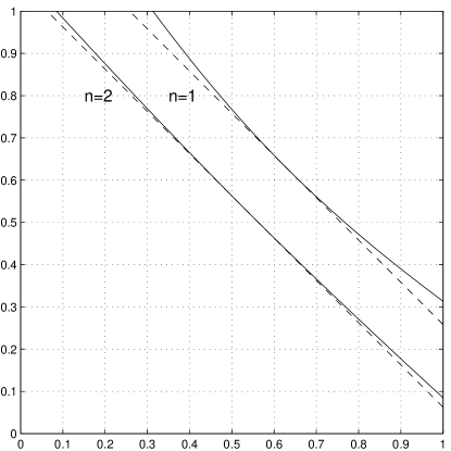
Figure 3: For any pair of orthogonal states $\rho_{0,1}$ on ${\cal H}_{2^{n}}\otimes{\cal H}_{2^{n}}$, there exists an LOCC POVM with probabilities $p_{0|0}$, $p_{1|1}$ above the curves shown for $n=1$ and $n=2$. The dashed lines are the simpler, weaker bound of Eq. (39).

In Appendix B, we give a proof of this Theorem using a Lagrange multiplier analysis, together with an alternative simple proof for the weaker result Eq. (39). This bound is not necessarily tight; the proof of Theorem 39 gives no indication of whether or not the right hand side of Eq. (38) could be larger. However, its approximate behavior, i.e. $p_{0|0}+p_{1|1}-1\geq\frac{1}{2^{O(n)}}$ is in accordance with our findings in Section III.

V Hiding Multiple Bits

In this section we will prove the security of hiding multiple bits bitwise with the scheme described in Section III. Let ${\bf b}=(b_{1},b_{2},\cdots,b_{k})$ be a $k$-bit string to be hidden. The hiding state is

$$\rho_{\bf b}^{(n)}=\bigotimes_{l=1}^{k}\rho_{b_{l}}^{(n)}\,.$$ (40)

Showing the security of the bitwise scheme is nontrivial. First, one of the hiding states $\rho_{1}^{(n)}$ is entangled (see Section VI), and the entanglement in part of the system may help decode the partial secret in the rest of the system. Second, joint measurement on all $k$ tensor product components may provide more information than a measurement on each component separately. The security of multiple-bit hiding is established using the symmetry of $\rho_{0}^{(n)}$ and $\rho_{1}^{(n)}$, as captured by their Werner-state representation (Eqs. (23) and (24)).

In the setup for hiding $k$ bits, each POVM element $M_{\bf i}$ has a $k$-bit index ${\bf i}$ and acts on ${\cal H}_{2^{nk}}\otimes{\cal H}_{2^{nk}}$. Since $\rho_{\bf b}^{(n)}$ is invariant under $({\cal T}_{U(2^{n})})^{\otimes k}$, $M_{\bf i}$ can be parametrized as

$$M_{\bf i}=\sum_{p=0}^{k}\sum_{{\bf m}:w_{h}({\bf m})=k-p}\alpha_{p,{\bf m}}^{\bf i}X_{\bf m}\,.$$ (41)

where $X_{\bf m}=\bigotimes_{l=1}^{k}H_{n}^{m_{l}}$ and $w_{h}({\bf m})$ is the Hamming weight of the $k$-bit string ${\bf m}$. Here $m_{l}$ denotes the $l$th bit of ${\bf m}$, $H_{n}^{0}=I$ and $H_{n}^{1}=H_{n}$. The number of $H_{n}$ in $X_{\bf m}$ is thus $w_{h}({\bf m})$. With this parametrization the trace preserving condition $\sum_{\bf i}M_{\bf i}=I$ implies that

$$\begin{array}[]{lr}\sum_{\bf i}\alpha^{\bf i}_{k,{\bf m}={\bf 0}}=1\,,&\forall{\bf m}\neq{\bf 0}\;\sum_{{\bf i}}\alpha_{p,{\bf m}}^{\bf i}=0\,.\end{array}$$ (42)

Next we consider the constraint $({\bf 1}\otimes T)[M_{\bf i}]\geq 0$. The partial transpose replaces the operator $H_{n}$ by $P_{+}=(|\Phi^{+}\rangle\langle\Phi^{+}|)^{\otimes n}$. Therefore we have

$$({\bf 1}\otimes T)[M_{\bf i}]=\sum_{p=0}^{k}\sum_{{\bf m}:w_{h}({\bf m})=k-p}A_{p,{\bf m}}^{\bf i}Y_{\bf m}\,,$$ (43)

where $Y_{\bf m}$ is a tensor product of the orthogonal projectors ${\bf 1}-P_{+}$ and $P_{+}$, such that $P_{+}$ occurs where the $k$-bit string ${\bf m}$ has a $1$. Here the coefficients $A_{p,{\bf m}}^{\bf i}$ are particular sums of the coefficients $\alpha_{p,{\bf m}}^{\bf i}$ of Eq. (41):

$$A_{p,{\bf m}}^{\bf i}=\sum_{p\leq l\leq k}\sum_{\stackrel{{\scriptstyle{\bf n}:w_{h}({\bf n})=k-l}}{{\wedge_{i}({\bar{n}}_{i}\vee m_{i})=1}}}\alpha_{l,{\bf n}}^{\bf i}\,.$$ (44)

The Boolean-logic condition on ${\bf n}$ in the summation, $\wedge_{i}({\bar{n}}_{i}\vee m_{i})=1$, can be expressed in ordinary language by saying that the string n must have 0s wherever the sting m has 0s. A necessary (and, in fact, sufficient) condition for the positivity of Eq. (43) is that these coefficients $A_{p,{\bf m}}^{\bf i}\geq 0$. When $p=k$, this implies that

$$A_{k,{\bf m}={\bf 0}}^{\bf i}=\alpha_{k,{\bf 0}}^{\bf i}\geq 0\,.$$ (45)

Together with Eq. (42) we obtain for all ${\bf i}$

$$0\leq\alpha_{k,{\bf 0}}^{\bf i}\leq 1\,.$$ (46)

We will bound the coefficients $\alpha_{p,{\bf n}}^{\bf i}$ for all ${\bf i}$, $p$ and ${\bf n}$. These upper and lower bounds,

$$L_{p}\leq\alpha_{p,{\bf n}}^{\bf i}\leq U_{p}\,,$$ (47)

will be obtained recursively as we decrease $p$ from $k$. The recurrence starts with $L_{k}=0$ and $U_{k}=1$, Eq. (46). Let us assume that we can determine $L_{p}$ for $p<k$. Then $U_{p}$ directly follows, using the second equation in Eq. (42): we have

$$\alpha_{p,{\bf n}}^{{\bf j}}=-\sum_{{\bf i}\neq{\bf j}}\alpha_{p,{\bf n}}^{\bf i}\leq-(2^{k}-1)L_{p}\,,$$ (48)

or $U_{p}=-(2^{k}-1)L_{p}$ for $p<k$. Then we need to determine $L_{p}$, which can be done using the PPT condition. We can express $A_{p,{\bf m}}^{\bf i}\geq 0$ as

$$\alpha_{p,{\bf m}}^{\bf i} \geq -\sum_{p<l\leq k}\sum_{\stackrel{{\scriptstyle{\bf n}:w_{h}({\bf n})=k-l}}{{\wedge_{i}(\bar{n}_{i}\vee m_{i})=1}}}\alpha_{l,{\bf n}}^{\bf i}$$ (49)

$$\geq -\sum_{p<l\leq k}U_{l}{k-p\choose l-p}\,.$$

Or, for $p<k$

$$L_{p}=-\sum_{p<l\leq k}U_{l}{k-p\choose l-p}\,,$$ (50)

so, in terms of $L_{l}$:

$$L_{p}=-1+(2^{k}-1)\sum_{p<l<k}L_{l}{k-p\choose l-p}\,.$$ (51)

This recursion can be solved, giving

$$L_{p}=-\sum_{l=1}^{k-p}(1-2^{k})^{l-1}\sum_{j=1}^{l}(-1)^{j}{l\choose j}j^{k-p}\,,$$ (52)

which can be rewritten in terms of the Sterling numbers of the second type, $\{{x\atop y}\}$, as

$$L_{p}=-\sum_{l=1}^{k-p}(2^{k}-1)^{l-1}l!\left\{{k-p\atop l}\right\}\,.$$ (53)

Let us consider the probabilities $p_{{\bf i}|{\bf b}}={\rm Tr}\,(M_{\bf i}\rho_{\bf b})$. Using the fact that ${\rm Tr}\,H_{n}={\rm Tr}\,H_{n}^{2}=1$, it can be shown that for ${\bf m}$ with Hamming weight $k-p$

$${\rm Tr}\;(X_{\bf m}\rho_{\bf b})=\frac{(-1)^{{\bf b}\cdot{\bf m}}}{2^{n(k-p)}}\,.$$ (54)

Thus

$$p_{{\bf i}|{\bf b}}=\sum_{p=0}^{k}\sum_{{\bf m}:w_{h}({\bf m})=k-p}\alpha_{p,{\bf m}}^{\bf i}\frac{(-1)^{{\bf b}\cdot{\bf m}}}{2^{n(k-p)}}\,,$$ (55)

or

$$p_{{\bf i}|{\bf b}}=\alpha_{k,{\bf 0}}^{\bf i}+\sum_{p=0}^{k-1}\sum_{{\bf m}:w_{h}({\bf m})=k-p}\alpha_{p,{\bf m}}^{\bf i}\frac{(-1)^{{\bf b}\cdot{\bf m}}}{2^{n(k-p)}}\,.$$ (56)

We bound the magnitude of the last term as

$$\left|\sum_{p=0}^{k-1}\sum_{{\bf m}:w_{h}({\bf m})=k-p}\alpha_{p,{\bf m}}^{\bf i}\frac{(-1)^{{\bf b}\cdot{\bf m}}}{2^{n(k-p)}}\right|$$

$$\hskip 12.91663pt\leq\Delta=(2^{k}-1)\sum_{p=0}^{k-1}{k\choose k-p}\frac{|L_{p}|}{2^{n(k-p)}}\,,$$ (57)

so we bound the conditional probabilities

$$\alpha_{k,{\bf 0}}^{\bf i}-\Delta\leq p_{{\bf i}|{\bf b}}\leq\alpha_{k,{\bf 0}}^{\bf i}+\Delta\,.$$ (58)

$\Delta$ enters the bound for the mutual information obtainable by Alice and Bob. Ideally we would like to use Eq. (58) to bound the retrievable attainable mutual information assuming an arbitrary probability distribution for the hiding states $\rho_{{\bf b}}^{(n)}$, as we did in the case of hiding a single bit. We do not know if the proof technique of Theorem 2 in Appendix A is applicable in the multiple-bit case, so we will have recourse to another method which provides a bound in the case of equal probabilities $p_{\bf b}=\frac{1}{2^{k}}$.

We first bound the total error probability

$$p_{e}=1-\sum_{\bf b}p_{\bf b}\,p_{{\bf b}|{\bf b}}=1-{1\over 2^{k}}\sum_{\bf b}p_{{\bf b}|{\bf b}}\,.$$ (59)

Using Eq. (58) we get

$$1-{1\over 2^{k}}\sum_{\bf b}(\alpha_{k,{\bf 0}}^{\bf b}+\Delta)\leq p_{e}\leq 1-{1\over 2^{k}}\sum_{\bf b}(\alpha_{k,{\bf 0}}^{\bf b}-\Delta)\,,$$ (60)

and, with Eq. (42), we obtain

$$1-{1\over 2^{k}}-\Delta\leq p_{e}\leq 1-{1\over 2^{k}}+\Delta\,.$$ (61)

With this bound on the error probability it is possible to bound the mutual information between the $k$ hidden bits ${\bf b}$ and a multi-outcome measurement by Alice and Bob, similarly to the single bit case, see Eq. (22). For a process such as Eq. (22) where $B$ and $\hat{B}$ are replaced by $k$ bit random variables ${\bf B}$ and $\hat{{\bf B}}$, it can be shown that the mutual information $I({\bf B}:Y)\leq H({\bf B})+\log(1-p_{e})$. Using Eq. (61), this implies that

$$I({\bf B}:Y)\leq{2^{k}\over\ln 2}\Delta\,.$$ (62)

Figure 4 shows an exact calculation of this bound as a function of $n$ and $k$. We can show that these bound curves have a simple form in the region of interest by a further examination of Eqs. (53) and (57). It is straightforward to demonstrate that, if $k\gg 1$, Eq. (53) is dominated by its final term, so that we can approximate

$$L_{p}\approx-(2^{k}-1)^{k-p-1}(k-p)!\,.$$ (63)

With this we can write Eq. (57) as

$$\Delta \approx \sum_{s=1}^{k}{k\choose s}{(2^{k}-1)^{s}\over 2^{ns}}s!$$ (64)

$$= k!\sum_{i=0}^{k-1}\left({2^{k}-1\over 2^{n}}\right)^{k-i}{1\over i!}\,.$$

It is easy to show that if $2^{n-k}\gg k$ then the last term in this sum dominates, so we obtain

$$\Delta\approx k2^{k-n}\,,$$ (65)

and Eq. (62) becomes

$$I({\bf B}:Y)\stackrel{{\scriptstyle\textstyle<}}{{\sim}}{k2^{2k-n}\over\ln 2}\,.$$ (66)

The curves shown in Fig. 4 are excellently approximated by this expression.

Figure 4: Contours of constant upper bound on $\log I({\bf B}:Y)$, Eq. (62), while varying $n$ (the vertical axis) and $k$ (the horizontal axis). The bound on $\log I({\bf B}:Y)$ is calculated using the expression for $\Delta$ in Eq. (57) with $L_{p}$ in Eq. (53).

This result shows that if we fix $k$, there always exists an $n$ large enough so that the information that Alice and Bob can gain is arbitrarily small. Equation (66) says that, for a given security parameter $I({\bf B}:Y)\leq\epsilon$, $n$ should grow, in the large $k$ limit, as

$$n(k)\rightarrow 2k+\log k+\log\log{\rm e}+\log(1/\epsilon)\,.$$ (67)

It is interesting to note that the above bound is much weaker than in the case when information is additive over the different bits hidden, which would imply

$$n(k)\rightarrow\log k+\log(1/\epsilon)\,.$$ (68)

Sufficient conditions for information to be additive will be discussed in Section VII-A.

VI Preparation of the hiding states

We consider the question of how the hider can efficiently produce the states $\rho_{0}^{(n)}$ and $\rho_{1}^{(n)}$ starting with minimal entanglement between the two shares. The defining representation of the states, Eqs. (3) and (4), suggests a method to create the hiding states by picking $n$ Bell states with the correct number of singlets (even or odd). This method is computationally efficient, but uses a lot of quantum entanglement between the shares, namely $n$ ebits per hiding state. The alternative representation of $\rho_{0}^{(n)}$ and $\rho_{1}^{(n)}$ as Werner states, Eqs. (23) and (24), can be used to show that they have $0$ and $1$ ebit of entanglement of formation respectively [18, 20]. We first describe an efficient LOCC preparation for $\rho_{0}^{(n)}$ from the unentangled pure state $|{\bf 0}\rangle=|0\rangle^{\otimes n}\otimes|0\rangle^{\otimes n}$. By efficient we mean that the number of quantum and classical computational steps scales as a polynomial in $n$, the number of qubits in each share. Then, using the recursive relations Eq. (26), and the preparation for $\rho_{0}^{(n)}$, we give a preparation for $\rho_{1}^{(n)}$ using exactly $1$ ebit for arbitrary $n$. Note that this is a tight construction in terms of entanglement, since $\rho_{1}^{(n)}$ has an entanglement of formation of 1 ebit.

VI-A Preparing $\rho_{0}^{(n)}$

Recall from Section III that the Full Twirl

$${\cal T}_{U(2^{n})}[\rho]=\frac{1}{\mbox{Vol}(U)}\int\,dU(U\otimes U)\,\rho\,(U^{\dagger}\otimes U^{\dagger})\,,$$ (69)

has only two linearly independent invariants $I$ and $H_{n}$, and it transforms any state to a Werner state. Moreover, note that

$${\rm Tr}({\cal T}_{U(2^{n})}[\rho]H_{n})={\rm Tr}(\rho{\cal T}_{U(2^{n})}^{\dagger}[H_{n}])={\rm Tr}(\rho H_{n})\,.$$ (70)

Hence, the Full Twirl transforms $\rho$ to a Werner state with the same overlap with $H_{n}$. From Eqs. (23) and (30), ${\rm Tr}\left(\rho_{0}^{(n)}H_{n}\right)=\frac{1}{2^{n}}$; this also equals ${\rm Tr}\left(|{\bf 0}\rangle\langle{\bf 0}|H_{n}\right)$ using Eq. (25). Hence,

$$\rho_{0}^{(n)}={\cal T}_{U(2^{n})}\left[|{\bf 0}\rangle\langle{\bf 0}|\right]\,,$$ (71)

and $\rho_{0}^{(n)}$ could be prepared by applying ${\cal T}_{U(2^{n})}$ to $|{\bf 0}\rangle$.

The Full Twirl, interpreted as the application of a random bilateral unitary, is not efficient to implement. Applying a unitary transformation selected at random is a hard problem: almost all unitary transformations take an exponential time in the number of qubits to accurately approximate [21]. In the following, we give an efficient implementation of the Full Twirl, first by showing that it is equivalent to randomizing over the Clifford group only, and second by providing methods to select and implement a random Clifford group element efficiently.

VI-A1 Clifford Twirl

The Clifford group ${\cal C}$ has appeared in quantum information theory as an important group in the context of quantum error correcting codes [22, 8]. The Clifford group ${\cal C}_{n}\subset U(2^{n})$ is the normalizer of the Pauli group ${\cal P}_{n}$. The order of the Clifford group acting on $n$ qubits is $|{\cal C}_{n}|=2^{n^{2}+2n+3}\Pi_{j=1}^{n}(4^{j}-1)$ [22].

It is useful to consider how each $c\in{\cal C}_{n}$ acts on ${\cal P}_{n}$ by conjugation. As the conjugation map is reversible, ${\cal C}_{n}$ is a subgroup of the permutation group acting on ${\cal P}_{n}$. Each $c$ is specified by the $2n$ images of the generators of ${\cal P}_{n}$ $a_{i}=c\sigma_{x}^{({i})}c^{\dagger}$ and $b_{i}=c\sigma_{z}^{({i})}c^{\dagger}$ for $i=1,\cdots,n$. There are restrictions on these images, since conjugation preserves the eigenvalues (and thus the trace), the commutation relations, and the multiplicative structure of the Pauli group. Because of eigenvalue preservation, conjugation preserves the hermitian subset $\tilde{\cal P}_{n}$ (introduced earlier, see Eq. (11)). The images are $2n$ traceless hermitian Pauli operators satisfying the commutation relations $\forall i,j$ $[a_{i},a_{j}]=[b_{i},b_{j}]=0$, $\forall i\neq j$ $[a_{i},b_{j}]=0$ and $\{a_{i},b_{i}\}=0$. Each $c\in{\cal C}_{n}$ can be explicitly constructed: first choose $a_{1}\neq I$, then choose $a_{2}$ to commute with $a_{1}$, and $a_{2}\notin\{I,a_{1}\}$, then choose $a_{3}$ to commute with $a_{1},a_{2}$ and $a_{3}\notin\{I,a_{1},a_{2},a_{1}a_{2}\}$, and so on until $a_{n}$ is chosen. Each $b_{i}$ can be chosen to anticommute with $a_{i}$ and commute with all other $a_{j}$ and $b_{1},\cdots,b_{i-1}$. If $(a_{1},\cdots,a_{n},b_{1},\cdots,b_{n})$ is a valid set of images corresponding to a Clifford group element $c$, $((-1)^{\epsilon_{1}}a_{1},\cdots,(-1)^{\epsilon_{n}}a_{n},(-1)^{\epsilon_{n+1}}b_{1},\cdots,(-1)^{\epsilon_{2n}}b_{n})$ is another valid set corresponding to

$$c\,(\sigma_{z}^{\epsilon_{1}}\sigma_{x}^{\epsilon_{n+1}}\otimes\ldots\otimes\sigma_{z}^{\epsilon_{n}}\sigma_{x}^{\epsilon_{2n}})\,,$$ (72)

where each $\epsilon_{i}=0,1$.

We define the “Clifford twirl” on ${\cal H}_{2^{n}}\otimes{\cal H}_{2^{n}}$ to be the operation

$${\cal T}_{{\cal C}_{n}}[\rho]=\frac{1}{|{\cal C}_{n}|}\sum_{c\in{\cal C}_{n}}(c\otimes c)\,\,\rho\,\,(c^{\dagger}\otimes c^{\dagger})\,.$$ (73)

We now prove that ${\cal T}_{{\cal C}_{n}}={\cal T}_{U(2^{n})}$. We need to show that these two quantum operations transform any state to the same output. It suffices to show that (1) ${\cal T}_{{\cal C}_{n}}={\cal T}_{{\cal C}_{n}}^{\dagger}$, (2) ${\cal T}_{{\cal C}_{n}}[I]=I$, (3) ${\cal T}_{{\cal C}_{n}}[H_{n}]=H_{n}$, and (4) ${\cal T}_{{\cal C}_{n}}$ transforms any state to a linear combination of $I$ and $H_{n}$. Conditions (1)-(4) ensure that ${\cal T}_{{\cal C}_{n}}$ transforms any state to a Werner state with the correct overlap with $H_{n}$, i.e., ${\rm Tr}\,(H_{n}\rho)={\rm Tr}\,(H_{n}{\cal T}_{{\cal C}_{n}}[\rho])$ (cf. Eq. (70)). Conditions (1) and (2) are obvious. Condition (3) can be proved by writing

$$H_{n} = \left(({\bf 1}\otimes T)[|\Phi^{+}\rangle\langle\Phi^{+}|]\right)^{\otimes n}$$ (74)

$$= {1\over 4^{n}}(I\otimes I+\sigma_{x}\otimes\sigma_{x}+\sigma_{y}\otimes\sigma_{y}+\sigma_{z}\otimes\sigma_{z})^{\otimes n}$$

$$= {1\over 2}{1\over 4^{n}}\sum_{P\in\tilde{\cal P}_{n}}P\otimes P\,.$$

Since conjugation by each $c\in{\cal C}_{n}$ only permutes the terms in this sum over $\tilde{\cal P}_{n}$, $H_{n}$ is invariant under ${\cal T}_{{\cal C}_{n}}$. This establishes (3).

To show condition (4), we consider the action of ${\cal T}_{{\cal C}_{n}}$ on a basis for the density matrices. We choose the basis $P_{1}\otimes P_{2}\in\tilde{\cal P}_{n}\otimes\tilde{\cal P}_{n}$. We already know that ${\cal T}_{{\cal C}_{n}}[I\otimes I]=I\otimes I$. Without loss of generality, $P_{1}\neq I$. First consider $P_{1}\neq P_{2}$. There exists a $\tilde{c}$ such that $\tilde{c}P_{1}\tilde{c}^{\dagger}=\sigma_{x}^{({1})}$ and $\tilde{c}P_{2}\tilde{c}^{\dagger}=g=\sigma_{x}^{({2})}$ or $\sigma_{z}^{({1})}$ or $I$ depending on whether $[P_{1},P_{2}]=0$ or $\{P_{1},P_{2}\}=0$ or $P_{2}=I$. Then

$${\cal T}_{{\cal C}_{n}}[P_{1}\otimes P_{2}] = \frac{1}{|{\cal C}_{n}|}\sum_{c\in{\cal C}_{n}}(cP_{1}c^{\dagger})\otimes(cP_{2}c^{\dagger})$$ (75)

$$= \frac{1}{|{\cal C}_{n}|}\sum_{c\in{\cal C}_{n}}(c\sigma_{x}^{({1})}c^{\dagger})\otimes(cgc^{\dagger})\,.$$

For every $c$, there is another $c^{\prime}$ (see Eq. (72)) such that $c^{\prime}\sigma_{x}^{({1})}c^{\prime\dagger}=-c\sigma_{x}^{({1})}c^{\dagger}$ and $c^{\prime}gc^{\prime\dagger}=cgc^{\dagger}$, hence the sum vanishes. Now consider $P=P_{1}\otimes P_{1}$.

$${\cal T}_{{\cal C}_{n}}[P_{1}\otimes P_{1}]=\frac{1}{|{\cal C}_{n}|}\sum_{c\in{\cal C}_{n}}(c\sigma_{x}^{({1})}c^{\dagger})\otimes(c\sigma_{x}^{({1})}c^{\dagger})\,.$$ (76)

Following the discussion on specifying Clifford group elements, $c\sigma_{x}^{({1})}c^{\dagger}$ ranges over all elements in $\tilde{\cal P}_{n}-\{I\}$. Moreover, each $c\sigma_{x}^{({1})}c^{\dagger}$ occurs in the sum the same number of times independent of $c$; this is the number of valid combinations $a_{2},\cdots,a_{n}$, $b_{1},\cdots,b_{n}$ that complete the image set, which is independent of $c$. Thus we obtain

$$P\otimes P\stackrel{{\scriptstyle{\cal T}_{{\cal C}_{n}}}}{{\rightarrow}}{1\over|\tilde{\cal P}_{n}|-1}\sum_{Q\in\tilde{\cal P}_{n}-\{I\}}Q\otimes Q\,.$$ (77)

Comparing this with Eq. (74), we see that this is a linear combination of $I$ and $H_{n}$. This proves condition (4), and thus ${\cal T}_{{\cal C}_{n}}={\cal T}_{U(2^{n})}$. Therefore ${\cal T}_{{\cal C}_{n}}[|{\bf 0}\rangle\langle{\bf 0}|]=\rho_{0}^{(n)}$.

VI-A2 Selecting and implementing a random element in the Clifford group

To implement the Clifford twirl efficiently, we need to select and implement random elements in the Clifford group. Our method is based on the circuit construction of any Clifford group element in Ref. [8] by Gottesman. The essence of his construction is as follows. We choose the following generating set for the Clifford group ${\cal C}_{n}$:

$$G=\{{\sc h}_{i},{\sc cnot}_{jk},{\sc p}_{m},{\sc p}^{\dagger}_{n}\}\,,$$ (78)

where h, cnot, and p respectively stand for the 1-qubit Hadamard transform $\frac{1}{\sqrt{2}}{1\,\,\,\,\,1\choose 1\,-1}$, the 2-qubit controlled-not, and the 1-qubit phase gate $1\,\,0\choose 0\,\,i$. Subscripts in Eq. (78) denote the qubit(s) being acted on.

Note that the generating set is self-inverse and that it has $n^{2}+2n$ elements. From Ref. [8], a circuit with no more than $3n^{2}+7n+O(1)$ gates from $G$ can be explicitly constructed for each element in ${\cal C}_{n}$.

It remains to find a method to select any random element in ${\cal C}_{n}$ with uniform probability. This cannot be done simply by randomizing the building blocks of the Gottesman construction. Hence we use a random walk over ${\cal C}_{n}$ to generate a random element, which can then be implemented by the Gottesman construction. Even though $|{\cal C}_{n}|$ is of order $2^{O(n^{2})}$, it can be proved that our random walk converges in $O(n^{8})$ steps to the uniform distribution over the Clifford group elements.

The algorithm can be summarized as follows:

1. Classical random walk.  Determine a random element using a random walk algorithm: at every time step, with probability $1/2$, do nothing, and with probability $1/2$ choose a random element in $G$. Proceed for $O(n^{8})$ steps. Let the resulting element be $U$. Classically compute the images $U\sigma_{x}^{({i})}U^{\dagger}$ and $U\sigma_{z}^{({i})}U^{\dagger}$, which can be done efficiently following the Knill-Gottesman theorem [8].

2. Quantum circuit.  Using the $2n$ images, build a quantum circuit to implement $U$ using the Gottesman construction with $3n^{2}+7n+O(1)$ generators.

Remarks: We separate the algorithm into classical and quantum parts because there are $O(n^{8})$ classical steps but only $O(n^{2})$ quantum gates. The ‘do nothing’ step with probability 1/2 is based on a technicality in the proof and may be skipped in an implementation, so that a random generator is picked at every round.

We prove that the Markov random walk ‘mixes’ in $O(n^{8})$ steps. The proof [23] relies on the facts that (1) any element of the Clifford group can be reached from any other by applying $O(n^{2})$ generators, i.e. the diameter $d$ of the (Cayley) graph of the group is $O(n^{2})$, and (2) the random walk uses a symmetric (self-invertible) set of generators over a group. We use Corollary 1 in Ref. [24] to bound the second largest eigenvalue $\lambda_{2}$ of this Markov chain as

$$\lambda_{2}\leq 1-\eta/d^{2}\,,$$ (79)

where $d$ is the diameter and $\eta$ is the probability of the least likely generator, which is $\eta=\frac{1}{n^{2}+2n}$ in our case. Therefore $\lambda_{2}\leq 1-O(1/n^{6})$. Then, using Lemma 2 in Ref. [24], after $k$ steps of iteration the distance of the obtained distribution $p^{(k)}$ from the uniform distribution $u(c)=\frac{1}{|{\cal C}|}$ is bounded as $||p^{(k)}-u||_{1}\leq\sqrt{|{\cal C}|}(1-O(1/n^{6}))^{k}$. Here, we use the $L_{1}$ norm between two distributions $p(c)$ and $q(c)$, i.e. $||p-q||_{1}=\sum_{c\in{\cal C}}|p(c)-q(c)|$. If we set $k=O(n^{8})$, this distance can be bounded by a small constant.

VI-B Preparing $\rho_{1}^{(n)}$

The state $\rho_{1}^{(n)}$ can be created using one singlet state. This is obvious when $n=1$. For $n\geq 2$, $\rho_{1}^{(n)}$ can be created using the recurrence relation Eq. (26) by the following recursive process:

• Flip a coin with bias $p_{n}$ for $0$, and bias $1-p_{n}$ for $1$.

• If the outcome is $0$, prepare $\rho_{0}^{(n-1)}\otimes\rho_{1}^{(1)}$. If the outcome is $1$, prepare $\rho_{1}^{(n-1)}\otimes\rho_{0}^{(1)}$. When $n-1\geq 2$, $\rho_{1}^{(n-1)}$ is prepared recursively. Otherwise, $\rho_{1}^{(n-1)}$ is just the singlet.

Note that the procedure relies on the preparation of all possible $\rho_{0}^{(n)}$ without entanglement. Note also that the singlet $\rho_{1}^{(1)}$ is used exactly once in the procedure.

VII Data hiding in separable states

We have considered hiding states with very little entanglement. In this section, we consider completely separable hiding states. Such “separable hiding schemes” are interesting for several reasons. First, given a separable scheme to hide one bit, multiple bits can be hidden bitwise; if the probability distributions of these bits are independent, then the attainable information is additive (as will be proved in Section VII-A). Second, the hiding states can be prepared without entanglement. Third, from a more fundamental perspective, such separable hiding schemes exhibit the intriguing phenomenon of quantum nonlocality without entanglement [5] to the fullest extent. We have good candidates for separable hiding states, but have not been able to prove their security rigorously. First we present a proof due to Wootters of the additivity of information in a bitwise application of separable hiding schemes.

VII-A Additivity of information when states are separable

Suppose the bit $b=0,1$ can be hidden in the separable states $\rho_{b=0,1}$, with bounded attainable mutual information, $I(B:Y)\leq\delta$. We call this the “single-bit protocol”. We consider hiding two bits $b_{1},b_{2}$ in the tensor-product state $\rho_{b_{1}}\otimes\rho_{b_{2}}$. Consider $I(B_{1}B_{2}:Y_{12})$ where $Y_{12}$ is the outcome of any measurement on $\rho_{b_{1}}\otimes\rho_{b_{2}}$ which is LOCC between Alice and Bob but can be jointly on $\rho_{b_{1}}$ and $\rho_{b_{2}}$. By the chain rule of mutual information [25], we have

$$I(B_{1}B_{2}:Y_{12})=I(B_{1}:Y_{12})+I(B_{2}:Y_{12}|B_{1})\,.$$ (80)

We now show that, when $b_{1}$ and $b_{2}$ are independent (having a product distribution $p(b_{1})p(b_{2})$), both $I(B_{1}:Y_{12})$ and $I(B_{2}:Y_{12}|B_{1})$ can be reinterpreted as the information obtained about a bit hidden with the single-bit protocol and are bounded by $\delta$. The term $I(B_{1}:Y_{12})$ measures how much about $b_{1}$ is learned from $Y_{12}$, when $b_{2}$ is unknown. This is also the information about $b_{1}$ learned from $\rho_{b_{1}}$ by the following LOCC procedure: First, append an extra $\rho_{b_{2}}$, chosen according to the probability distribution $p(b_{2})$. Then, without using their knowledge of $b_{2}$, Alice and Bob measure $Y_{12}$ on $\rho_{b_{1}}\otimes\rho_{b_{2}}$. Thus $I(B_{1}:Y_{12})\leq\delta$. It is crucial that $\rho_{b_{2}}$ is separable and can thus be prepared by LOCC. Similarly, $I(B_{2}:Y_{12}|B_{1})$ is the information about $b_{2}$ learned from $\rho_{b_{2}}$ by appending a known extra $\rho_{b_{1}}$ (chosen with probability $p(b_{1})$) and measuring $Y_{12}$. Hence $I(B_{2}:Y_{12}|B_{1})\leq\delta$. More generally, $I(B_{1}B_{2}\cdots B_{k}:Y)\leq k\delta$ for any $Y$, implying that the information is additive.

Note that this additive information bound for separable hiding states is much stronger than that for entangled hiding states (Section V). Note that there is an important difference between hiding with separable states and the problem of classical data transmission through a (noisy) quantum channel. For the latter it is known that the capacity is nonadditive, in the sense that the receiver has to perform joint measurements on the data to retrieve the full Holevo information [26]. The difference is that to achieve the Holevo information one encodes the classical data, so that the prior distribution is not independent over the different states. In our information bound for bit hiding, the different bits are assumed to have independent prior probabilities.

VII-B An alternative hiding scheme

In this section, we discuss some interesting properties of two orthogonal separable states in ${\cal H}_{2}\otimes{\cal H}_{2}$, and a candidate separable hiding scheme built from them. Consider the following two bipartite states in ${\cal H}_{2}\otimes{\cal H}_{2}$, introduced in Section VII of [5]:

$$\tau_{0}=\frac{1}{2}\left[\rule{0.0pt}{9.04166pt}\right.|+\rangle\langle+|\otimes|0\rangle\langle 0|+|0\rangle\langle 0|\otimes|+\rangle\langle+|\left.\rule{0.0pt}{9.04166pt}\right]\,,$$

$$\tau_{1}=\frac{1}{2}\left[\rule{0.0pt}{9.04166pt}\right.|-\rangle\langle-|\otimes|-\rangle\langle-|+|1\rangle\langle 1|\otimes|1\rangle\langle 1|\left.\rule{0.0pt}{9.04166pt}\right]\,,$$ (81)

where $|\pm\rangle={1\over\sqrt{2}}(|0\rangle\pm|1\rangle)$. These separable states are orthogonal, but the results of Ref. [5] suggest that they are not perfectly distinguishable by LOCC. We now strengthen this result using the general framework for LOCC measurements described in Section II.

Our goal as before is to bound $p_{0|0}+p_{1|1}$ obtained by any measurement with PPT POVM elements. Following the discussion of Section II, we restrict to PPT POVM elements $M_{0,1}$, and use the symmetry of $\tau_{0,1}$ to simplify the possible form of $M_{0,1}$. It will suffice to consider POVM elements ${\cal T}^{\dagger}[M_{i}]$, where ${\cal T}[\rho]={1\over 4}(\rho+{\sc s}\rho{\sc s}+{\sc h}_{2}\rho{\sc h}_{2}+{\sc s}{\sc h}_{2}\rho{\sc h}_{2}{\sc s})$ with ${\sc h}_{2}={\sc h}\otimes{\sc h}$ being the bitwise Hadamard transformation on both qubits, and s being the swap operation on the two qubits. It is immediate that $\cal T$ is self-adjoint, and that it fixes $\tau_{0,1}$. Unlike in Section II, $\cal T$ is not LOCC, but it does preserve the PPT property of $M_{i}$, because ${\sc s}M_{i}{\sc s}$ is PPT (the swap just relabels the input bits). Moreover, $\forall M$, ${\cal T}[{\cal T}[M]]={\cal T}[M]$; therefore, we can restrict to POVM elements $M$ that are invariant under ${\cal T}$. This symmetry is most easily imposed in the Pauli decompositions of $M_{0,1}$:

$$M_{0} = aP_{a}+cP_{c}+eP_{e}+dP_{d}\,,$$

$$M_{1} = (1-a)P_{a}-cP_{c}-eP_{e}-dP_{d}\,,$$ (82)

where

$$P_{a} = I\otimes I\,,$$

$$P_{c} = \sigma_{z}\otimes I+I\otimes\sigma_{z}+\sigma_{x}\otimes I+I\otimes\sigma_{x}\,,$$

$$P_{d} = \sigma_{z}\otimes\sigma_{z}+\sigma_{x}\otimes\sigma_{x}\,,$$

$$P_{e} = \sigma_{z}\otimes\sigma_{x}+\sigma_{x}\otimes\sigma_{z}\,,$$ (83)

are the only linearly independent invariants under ${\cal T}$. Note that $M_{0,1}$ are automatically invariant under partial transpose. Therefore, it only remains to impose conditions on $a,c,d,e$ to make $0\leq M_{0}\leq I$:

$$0\leq a-2d\leq 1\,,$$ (84)

$$0\leq a-2e\leq 1\,,$$ (85)

$$0\leq\alpha\pm\beta\leq 1\,.$$ (86)

In Eqs. (84)-(86), the bounded quantities are eigenvalues of $M_{0}$, with $\alpha=a+d+e$ and $\beta=\sqrt{8c^{2}+(d-e)^{2}}$.

To find $p_{0|0}$ and $p_{1|1}$, we express $\tau_{0,1}$ in their Pauli decompositions, using $|0\rangle\langle 0|={1\over 2}(I+\sigma_{z})$, $|1\rangle\langle 1|={1\over 2}(I-\sigma_{z})$, and $|\pm\rangle\langle\pm|={1\over 2}(I\pm\sigma_{x})$:

$$\tau_{0}={1\over 8}(2P_{a}+P_{c}+P_{e})\,,$$

$$\tau_{1}={1\over 8}(2P_{a}-P_{c}+P_{d})\,.$$ (87)

Using Eqs. (82) and (87), and the trace orthonormality of the Pauli matrices (up to a multiplicative constant), we find the conditional probabilities of interest:

$$p_{0|0}=\mbox{Tr}(M_{0}\tau_{0}) \!\!\!\!=a+2c+e\,,$$ (88)

$$p_{1|1}=\mbox{Tr}(M_{1}\tau_{1}) \!\!\!\!=(1-a)+2c-d\,.$$

Figure 5: $(p_{0|0}^{(1)},p_{1|1}^{(1)})$ attainable by PPT-preserving measurements on $\tau_{0,1}$.

The values of $(p_{0|0},p_{1|1})$ permitted by the positivity constraints Eqs. (84)-(86) are depicted in Fig. 5; we leave the straightforward derivation of Fig. 5 to the interested reader. Here we only use Eq. (86) to derive a simple bound on $\left|p_{0|0}+p_{1|1}-1\right|$ (the straight portion of the boundary). We have:

$$\left|p_{0|0}+p_{1|1}-1\right| = 4c+(e-d)$$ (89)

$$= \sqrt{3}\,|\beta|\left|\rule{0.0pt}{12.91663pt}\right.\!\sqrt{{2\over 3}}{\sqrt{8}c\over|\beta|}+{1\over\sqrt{3}}{(e-d)\over|\beta|}\!\left.\rule{0.0pt}{12.91663pt}\right|\,.$$

Since $\beta=\sqrt{8c^{2}+(d-e)^{2}}$, the last factor in the last line is of the form $|\cos\theta\cos\phi+\sin\theta\sin\phi|=|\cos(\theta-\phi)|\leq 1$. Moreover, from Eq. (86), $|\beta|\leq{1\over 2}$. Hence,

$$\left|p_{0|0}+p_{1|1}-1\right|\leq{\sqrt{3}\over 2}\,.$$ (90)

This upper bound for protocols with the P-H property is tight, in the sense that there exists a simple LOCC procedure that achieves this bound. This procedure is described in Appendix C.

Equation (90) establishes that $\tau_{0,1}$ cannot be perfectly distinguished by measurements with PPT POVM elements, since the perfect measurement would give $p_{0|0}+p_{1|1}=2$. We can also put a lower bound on the amount of entanglement required to distinguish $\tau_{0}$ from $\tau_{1}$ perfectly. The combined support of $\tau_{0}$ and $\tau_{1}$ has full rank and $\tau_{0}$ and $\tau_{1}$ are orthogonal; therefore, the perfect POVM measurement has unique $M_{0,1}$. The measurement, if used as in Fig. 1(b), can create the states $M_{0}/{\rm Tr}(M_{0})$ and $M_{1}/{\rm Tr}(M_{1})$. These both have $\approx 0.55$ ebits of entanglement of formation, as calculated using Ref. [27]. Therefore, $\tau_{0,1}$ take at least $0.55$ ebits to distinguish perfectly.

We conjecture that the parity of the number of $\tau_{1}$ in a tensor product of $n$ $\tau_{0}$s and $\tau_{1}$s cannot be decoded better than by measuring each tensor component and combining the results. More precisely, we consider distinguishing the states

$$\tau_{b}^{(n)}={1\over 2^{n-1}}\sum_{b_{1}\oplus b_{2}\oplus\cdots\oplus b_{n}=b}\tau_{b_{1}}\otimes\tau_{b_{2}}\otimes\cdots\otimes\tau_{b_{n}}\,.$$ (91)

Here $\oplus$ is addition modulo two. We follow the general method to find the allowed values of $(p_{0|0}^{(n)},p_{1|1}^{(n)})$, and consider PPT $M_{0,1}\geq 0$ with the proper symmetries. Since the eigenvalues of $M_{0}$ for $n\geq 2$ are not analytically obtainable, we have performed a numerical maximization of $p_{1|1}^{(n)}$ with fixed $p_{0|0}^{(n)}$ for $n=2$ and $n=3$. All numerical results presented have negligible numerical errors. The allowed region for $(p_{0|0}^{(2)},p_{1|1}^{(2)})$ is given in Fig. 6.

Figure 6: $(p_{0|0}^{(2)},p_{1|1}^{(2)})$ attainable by PPT-preserving measurements on $\tau_{0,1}$.

The best value of $p_{0|0}^{(2)}+p_{1|1}^{(2)}$ is precisely the one achieved by applying the LOCC measurement in Appendix C on each tensor component, and classically combining the results to infer the parity. The same has been confirmed for $n=3$: $p_{0|0}^{(3)}+p_{1|1}^{(3)}\leq 1.64952$. While we have no convincing arguments for the conjecture for general $n$, the $n=2,3$ cases are unlikely to be degeneracies or coincidences.

Suppose the conjecture is true. Let ${1\over 2}(p_{0|0}^{(1)}+p_{1|1}^{(1)})\leq p$ where $p={1\over 2}+{\sqrt{3}\over 4}$ denotes the best decoding probability for $n=1$. Then, $\tau_{b}^{(n)}$ is distinguished correctly only if an even number of components are decoded incorrectly, thus

$$p_{0|0}^{(n)}+p_{1|1}^{(n)} \leq 2\sum_{k~{}{\rm even}}p^{n-k}(1-p)^{k}{n\choose k}$$ (92)

$$= (p+(1-p))^{n}+(p-(1-p))^{n}$$

$$= 1+(2p-1)^{n}$$

$$= 1+\left(\rule{0.0pt}{10.33327pt}\right.\!{\sqrt{3}\over 2}\!\left.\rule{0.0pt}{10.33327pt}\right)^{n}\,.$$

The upper bound on $p_{0|0}^{(n)}+p_{1|1}^{(n)}-1$ implies $\left|\rule{0.0pt}{9.04166pt}\right.\!\!p_{0|0}^{(n)}+p_{1|1}^{(n)}-1\!\!\left.\rule{0.0pt}{9.04166pt}\right|\leq\left(\rule{0.0pt}{9.04166pt}\right.\!\!{\sqrt{3}\over 2}\!\!\left.\rule{0.0pt}{9.04166pt}\right)^{n}$. If the conjecture is true, this bound vanishes exponentially with the number of qubits used, and $\tau_{b}^{(n)}$ can be used to hide a single bit in a way similar to the Bell mixtures $\rho_{b}^{(n)}$. Comparing Eqs. (92) and (34), the separable scheme takes ${1\over 1-\log_{2}\sqrt{3}}\approx 4.8$ times as many qubits as in the Bell-state protocol to achieve the same level of security.

VIII Conditionally Secure Quantum Bit Commitment

Bit commitment [28] is a cryptographic protocol with two parties, Alice and Bob. It has two stages, the commit and the open phases. The goal is to enable Alice to commit to a bit that can neither be learned by Bob before the open phase nor be changed by Alice after the commit phase. Bit commitment is a primitive for many other protocols, such as coin tossing, cf. Ref. [28]. However, the security of classical bit commitment schemes relies on unproved assumptions on computational complexity, while unconditionally secure quantum bit commitment has been proved to be impossible [29, 30].

In this section, we use the main idea of the bit hiding scheme in Section III to construct a conditionally secure bit commitment scheme in the following setting. The commitment is shared between two recipients (Bob-1 and Bob-2) who do not share entanglement and can perform only LOCC. Thus the present discussion contrasts with previous works in that (1) it is not precisely a two-party protocol and (2) the security is conditioned on restricting the two Bobs to LOCC operations only.

Let $n,r$ be security parameters. The scheme is secure in the sense that the dishonest Bobs learn at most $2^{-(n-1)}$ bits on the committed bit before the open phase, and a dishonest Alice can change her commitment without being caught with probability $2^{-r}$. The scheme is as follows:

• Commit phase: To commit to $b=0$ ($b=1$), Alice picks a random $|w_{\bf k}\rangle$ with an even (odd) number of singlets $|w_{11}\rangle$. Alice sends one qubit of each Bell pair to each Bob.

• Open phase: Alice sends $n+r$ singlets to Bob-1 and Bob-2, who apply a random hashing test [7, 31] and use $r$ of the singlets to check if the received states are indeed singlets. Alice is declared cheating if the test fails. Otherwise, the remaining $n$ singlets are used to teleport Bob-1’s qubits to Bob-2 who measures k to find $b$.

Proof:

If Alice is honest, the security of the bit hiding scheme implies that the dishonest Bobs can learn at most $O(2^{-n})$ bits of information before the open phase. If Bob is honest, the most general strategy for a dishonest Alice is to prepare a pure state $|\psi\rangle$ with five parts, $P_{i}$ for $i=1,\cdots,5$. In the commit phase, she gives $P_{1}$ and $P_{2}$ to Bob-1 and Bob-2. In the open phase, she applies some quantum operation $\cal E$ on $P_{3},P_{4},P_{5}$. Then, she sends $P_{3}$ and $P_{4}$ to Bob-1 and Bob-2. If $P_{3},P_{4}$ are indeed $n+r$ singlets, the test is passed and $\cal E$ does not change the state of $P_{1}$ and $P_{2}$, and Bob-2 indeed obtains $P_{1},P_{2}$ in the same state as in the commit phase after teleportation. ($P_{1},P_{2}$ can only be changed during the teleportation steps when interacting with $P_{3},P_{4}$ if they are not singlets.) In this case, the distribution of k and therefore the committed bit $b$ in both phases are the same – Alice cannot change or delay her commitment. In case $P_{3}$ and $P_{4}$ are not singlet states the analysis of the failure probability of the random hashing method follows the quantum key distribution security proof by Lo and Chau [31]. If $P_{3},P_{4}$ are in some state orthogonal to $n+r$ singlets, the test is passed with probability $2^{-r}$ only. In general, let $\alpha$ be the fidelity of $P_{3},P_{4}$ with respect to $n+r$ singlets. The probability to change the commitment without being caught is $\leq 2^{-r}(1-\alpha)$ which is less than $2^{-r}$.

∎

Note that our scheme does not force Alice to commit. For example, she can send an equal superposition of the $b=0,1$ states, but she cannot control the outcome at the opening phase. However, this is inherent to schemes which conceal the commitment from Bob. Classically, it is as if Alice sent an empty locked box with no bit written inside, or a device in which Bob’s opening the box triggered a fair coin toss to determine the bit.

We note that the above scheme has many equivalent variations. For example, Alice may instead prepare a superposition $\sum_{{\bf k}\in E_{n}/O_{n}}|\bf k\rangle\otimes|w_{\bf k}\rangle$ and send the second part to the Bobs, which provides a way of sending the density matrices $\rho_{b}^{(n)}$. Bob can request Alice to announce k in the open phase, and declare her cheating if he finds a different k. However, these schemes are exactly equivalent to the proposed one.

IX Discussion

The quantum data hiding protocol using Bell mixtures can be demonstrated with existing quantum optics techniques. The hider can prepare any one of the four polarization Bell states, $\frac{1}{\sqrt{2}}(|\updownarrow\,,\updownarrow\rangle\pm|\leftrightarrow\,,\leftrightarrow\rangle)$, $\frac{1}{\sqrt{2}}(|\updownarrow\,,\leftrightarrow\rangle\pm|\updownarrow\,,\leftrightarrow\rangle)$. Any of these can be prepared using downconversion [32], followed by an appropriate single photon operation. The photons can be sent through two different beam paths to Alice and Bob. Then Alice and Bob might attempt to unlock the secret by LOCC operations as in Section III-C; this requires high efficiency single-photon detection. Alternatively, the secret can be completely unlocked if a quantum channel is opened up for Alice to send her photons to Bob, who performs an incomplete measurement on each pair to distinguish the singlet $\frac{1}{\sqrt{2}}(|\updownarrow\,,\leftrightarrow\rangle-|\updownarrow\,,\leftrightarrow\rangle)$ from the other three Bell states. Such an incomplete measurement has been performed in the lab [32]; a full Bell measurement is not necessary and is in fact not technologically feasible in current experiments.

Our alternative low-entanglement preparation scheme would require more sophisticated quantum-optics technologies than presently exist but is interesting to consider. As we showed in Section VI, quantum operations in the Clifford group are required. The one-qubit gates are obtainable by linear optics, but the cnot gate cannot be implemented perfectly by using linear optical elements. However, recent work by Knill et al. [34] shows that a cnot gate can be implemented near-deterministically in linear optics when single-photon sources are available. So, this preparation scheme may be practicable in the near future as well.

We have proved for the Bell mixtures $\rho_{0,1}^{(n)}$ that the secret is hidden against LOCC measurements; but the secret can be perfectly unlocked by LOCC operations if Alice and Bob initially share $n$ ebits of entanglement (the LOCC procedure is just quantum teleportation followed by a Bell measurement by Bob). What is the smallest amount of entanglement $E_{min}$ required for perfect unlocking? This quantity would give another interesting measure of the strength of hiding. We do not know $E_{min}$ exactly, although we can give a lower bound for it. The bound is obtained by considering the procedure of Fig. 1(b) as a state-preparation protocol. Here we take the measurement M to be the nonlocal one that exactly distinguishes the hiding states. This M is unique because $\rho_{0,1}^{(n)}$ have full combined support and are orthogonal. Considering M to be an LOCC measurement performed with the assistance of $E_{min}$ ebits of prior entanglement, the average output entanglement of formation of Fig. 1(b) provides a lower bound for $E_{min}$, since the LOCC procedure cannot increase the average entanglement.

This entanglement of formation is straightforward to compute: When the input is two halves of two maximally entangled states as shown, the input density matrix, which is proportional to the identity, can be expressed as:

$${I\over 4^{n}}={|E_{n}|\over 4^{n}}\rho_{0}^{(n)}+{|O_{n}|\over 4^{n}}\rho_{1}^{(n)}\,.$$ (93)

The output state is therefore $\rho_{0,1}^{(n)}$ with probabilities ${|E_{n}|\over 4^{n}}$, ${|O_{n}|\over 4^{n}}$. Since the entanglement of formation of $\rho_{1}^{(n)}$ is 1 ebit, the average output entanglement of formation is ${|O_{n}|\over 4^{n}}={1\over 2}(1-2^{-n})$ ebits. Thus, $E_{min}\geq{1\over 2}(1-2^{-n})$. This is still far from the upper bound of $n$ ebits; considering more general input states in Fig. 1(b) could improve our lower bound.

Our technique of putting bounds on the capabilities of LOCC operations using the Peres-Horodecki criterion is an application of the work of Rains [35, 36]. He introduced a class of quantum operations that contains the LOCC class, which he called the p.p.t. superoperators [35, 36]; $\cal S$ is in the p.p.t. class iff $({\bf 1}\otimes T)\circ{\cal S}\circ({\bf 1}\otimes T)$ is a completely positive map. It has been proved that the p.p.t. class is identical to the class of quantum operations that have the Peres-Horodecki property, which we introduce in Section II.

This p.p.t. class also extends in a very precise way to the POVMs, in the following sense: the condition that all $M_{i}$ be PPT is both a necessary and sufficient condition for a POVM to have the P-H property (which is equivalent to saying that the POVM, viewed as a quantum operation from ${\cal H}_{d}\otimes{\cal H}_{d}$ to a one-dimensional space ${\cal H}_{1}\otimes{\cal H}_{1}$, is p.p.t.). The necessary part is proved in Section II; sufficiency can be derived by considering an arbitrary input $\rho$ to the POVM M including ancillas (as in Fig. 1(b), but with general input). The output density matrix for outcome $i$ is proportional to $\rho_{i}\propto{\rm Tr}_{p}(M_{i}\rho)$, where the partial trace is over the input Hilbert space to M. The partial transpose of this operator can be written $({\bf 1}\otimes T)[\rho_{i}]\propto{\rm Tr}_{p}[({\bf 1}\otimes T)[M_{i}]({\bf 1}\otimes T)[\rho]]$; the proof follows straightforwardly from this formula.

It should be noted that the symmetrizing operation ${\cal T}^{\dagger}$ introduced in Section II is not restricted to the p.p.t. class. For example, ${\cal T}^{\dagger}$ in Section VII-B is not in the p.p.t. class. ${\cal T}^{\dagger}$ only needs to be unital and has the property that ${\cal T}^{\dagger}[M]$ is PPT if $M$ is PPT. The latter resembles, but is very different from the P-H property, which also requires $({\bf 1}\otimes{\cal T}^{\dagger})[M]$ to be PPT if $M$ is PPT. The difference is reminiscent of the distinction between positive and completely positive maps.

We believe that our quantum data hiding scheme using Bell states can be extended to multiple parties. Consider for example the extension to three parties Alice, Bob and Charlie, who are restricted to carrying out LOCC operations amongst each other. Candidates for the hiding states are the 3-party extensions of the Werner states, studied by Eggeling and Werner [37].

X Acknowledgments

We thank Charles Bennett for the suggestion to consider data hiding with the separable $\tau$ states and discussions on hiding with Bell states and quantum bit commitment. We thank Bill Wootters for discussions and insights about the additivity of information in the case of hiding in separable states. We thank Vittorio Castelli for giving the proof relating error probability and mutual information which we use in bounding the attainable information about multiple bits. We thank Don Coppersmith, Greg Sorkin and Dorit Aharonov for discussion and for pointing out the relevant literature on random walks on Cayley graphs with a small diameter. We thank John Smolin for discussion and for writing the initial program for the numerical work described in Section VII. We acknowledge support from the National Security Agency and the Advanced Research and Development Activity through the Army Research Office contract number DAAG55-98-C-0041.

Appendix A Bounding the obtainable mutual information

Let $X$ be a binary random variable. Define $Z_{s}$ to be the set of all binary random variables that satisfy the following bound on the conditional probabilities:

$$-\delta\leq p(Z=0|X=0)+p(Z=1|X=1)-1\leq\delta\,,$$ (94)

as in Eq. (21). Define $Y_{s}$ as the set of all random variables, with any number of outcomes, for which all “decoding processes” ${\cal D}$ produce binary random variables in the set $Z_{s}$. This situation is summarized as

$$X\stackrel{{\scriptstyle{\cal M}}}{{\rightarrow}}Y\stackrel{{\scriptstyle{\cal D}}}{{\rightarrow}}Z\,.$$ (95)

Note that $p(Z|Y)$ prescribed by $\cal D$ may depend on $p(Y|X)$. In this setting, we have the following bound:

Theorem 2

$\forall Y\in Y_{s},\ \ I(X:Y)\leq\delta H(X)$.

Proof:

We first derive bounds on the conditional probability distribution of any $Y\in Y_{s}$ given $X$. We consider $p(Z\!=\!k|X\!=\!l)=\sum_{j}p_{{\cal D}}(Z\!=\!k|Y\!=\!j)p(Y\!=\!j|X\!=\!l)$ implied by any $Y$ and $\cal D$. When we maximize $I(X:Y)$ over $Y$ with fixed ${\cal D}$, we obtain an overestimate of $I(X:Y)$ because we can maximize $Y$ over a superset of $Y_{s}$. Hence we can focus on a particular decoding process ${\cal D}$ defined as:

$$p_{\cal D}(Z\!=\!0|Y\!=\!j)=1 {\rm if} j\in I_{0}\cup I_{-}\,,$$

$$p_{\cal D}(Z\!=\!1|Y\!=\!j)=1 {\rm if} j\in I_{+}\,,$$ (96)

where

$$j\in I_{+}\Leftrightarrow p(Y\!=\!j|X\!=\!1)>p(Y\!=\!j|X\!=\!0)\,,$$

$$j\in I_{0}\Leftrightarrow p(Y\!=\!j|X\!=\!1)=p(Y\!=\!j|X\!=\!0)\,,$$

$$j\in I_{-}\Leftrightarrow p(Y\!=\!j|X\!=\!1)<p(Y\!=\!j|X\!=\!0)\,.$$ (97)

Given these we can compute

$$p(Z\!=\!0|X\!=\!0)+p(Z\!=\!1|X\!=\!1)$$ (98)

$$= \!\!\!\!\!\sum_{j\in I_{0}\cup I_{-}}p(Y\!=\!j|X\!=\!0)\!+\!\sum_{j\in I_{+}}p(Y\!=\!j|X\!=\!1)\hskip 51.6665pt$$

$$= \sum_{j}\max(p(Y\!=\!j|X\!=\!0),p(Y\!=\!j|X\!=\!1))\hskip 51.6665pt$$

$$= \!\!1\!+\!\sum_{j\in I_{+}}p(Y\!=\!j|X\!=\!1)-p(Y\!=\!j|X\!=\!0)\,.$$

Substituting Eq. (98) into Eq. (94), the first inequality becomes trivial and the second inequality gives a necessary condition on the set $Y_{s}$:
$~{}~{}\forall Y\in Y_{s}$,

$$\sum_{j\in I_{+}}p(Y\!=\!j|X\!=\!1)-p(Y\!=\!j|X\!=\!0)\leq\delta\,.$$ (99)

We now use Eq. (99) to bound $I(X:Y)$. We introduce the notations $p_{j0}=p(Y\!=\!j|X\!=\!0)$ and $p_{j1}=p(Y\!=\!j|X\!=\!1)$ for the conditional probabilities, and $p(X\!=\!0)=x_{0}$ and $p(X\!=\!1)=x_{1}=1-x_{0}$ for the fixed prior probabilities for $X$. We can then write the mutual information as

$$I(X:Y)=\sum_{j\in I_{+}\cup I_{-}}f(p_{j0},p_{j1})$$ (100)

where (101)

$$f(p_{j0},p_{j1})=\sum_{\alpha=0}^{1}x_{\alpha}p_{j\alpha}\log{p_{j\alpha}\over x_{0}p_{j0}+x_{1}p_{j1}}$$

represents the information on $X$ obtained from the outcome $Y\!=\!j$, weighted by $p(Y\!=\!j)$. Note also the outcomes in $I_{0}$ do not contribute to the mutual information. We will maximize Eq. (101) subject to the constraints

$$\sum_{j}p_{j0}=1\,,~{}~{}~{}\sum_{j}p_{j1}=1\,,$$ (102)

and

$$\sum_{j\in I_{+}}p_{j1}-p_{j0}\leq\delta\,.$$ (103)

The maximization of $I(X:Y)$ is made tractable by noting that any optimal $Y$ can be replaced by another $Y^{\prime\prime}$ with $|I^{\prime\prime}_{+}|,|I^{\prime\prime}_{0}|,|I^{\prime\prime}_{-}|\leq 1$, and satisfying the same constraints Eqs. (102) and (103). We prove this using the fact that $f(p_{0},p_{1})=f({\vec{p}})$ is linear ($f(c{\vec{p}})=cf({\vec{p}})$) and convex, giving

$$f(c_{0}\,{\vec{p}}+c_{1}\,{\vec{q}}) \leq c_{0}f({\vec{p}})+c_{1}f({\vec{q}})$$ (104)

$$= f(c_{0}\,{\vec{p}})+f(c_{1}\,{\vec{q}})\,.$$

Absorbing the nonnegative factors $c_{0,1}$ into the probability vectors, this becomes simply

$$f({\vec{p}}+{\vec{q}})\leq f({\vec{p}})+f({\vec{q}})\,.$$ (105)

The convexity of $f$ is proved by showing that the Hessian matrix $\partial^{2}f/\partial p_{\alpha}\partial p_{\beta}$ is positive semidefinite (it is straightforward to show that its eigenvalues are $0$ and $x_{0}x_{1}(p_{0}^{2}+p_{1}^{2})/(p_{0}p_{1}\sum_{\alpha}x_{\alpha}p_{\alpha})$).

Given any $Y$, we first construct an intermediate $Y^{\prime}$ as follows: For each outcome $j\in Y$ with unequal conditional probabilities $(p_{j0},p_{j1})$, introduce two outcomes in $Y^{\prime}$ with conditional probabilities:

$$(0,p_{j1}-p_{j0})~{}\mbox{and}~{}(p_{j0},p_{j0})~{}~{}~{}\mbox{if}~{}~{}~{}j\in I_{+}\,\,$$

$$(p_{j0}-p_{j1},0)~{}\mbox{and}~{}(p_{j1},p_{j1})~{}~{}~{}\mbox{if}~{}~{}~{}j\in I_{-}\,.$$

All outcomes in $I_{0}$ occur in $Y^{\prime}$ unchanged. Note that the number of outcomes are such that $|I^{\prime}_{\pm}|=|I_{\pm}|$ and $|I^{\prime}_{0}|=|I_{+}|+|I_{-}|+|I_{0}|$. The constraints Eqs. (102) and (103) are satisfied by $Y^{\prime}$ because the quantities involved are conserved by construction. $I(X:Y^{\prime})\geq I(X:Y)$ by applying Eq. (105) to each replacement. Finally, as all $I^{\prime}_{+}$ outcomes have $p_{j0}=0$, and all $I^{\prime}_{-}$ outcomes have $p_{j1}=0$, we introduce the desired random variable $Y^{\prime\prime}$ with just three outcomes, with conditional probabilities $(0,\sum_{j\in I^{\prime}_{+}}p_{j1})$, $(\sum_{j\in I^{\prime}_{-}}p_{j0},0)$, and $(\sum_{j\in I^{\prime}_{0}}p_{j0},\sum_{j\in I^{\prime}_{0}}p_{j0})$. $Y^{\prime\prime}$ still satisfies Eqs. (102) and (103), and the linearity of $f$ implies $I(X:Y^{\prime\prime})=I(X:Y^{\prime})$.

So, we have established that there exists an optimal $Y$ with conditional probabilities $(p_{10},0)$, $(0,p_{21})$, and $(p_{30},p_{30})$; these may be interpreted as the “certainly 0”, “certainly 1”, and “don’t know” outcomes. It is now trivial to show that the best choice of these parameters consistent with the constraints is given by $p_{10}=p_{21}=\delta$, $p_{30}=1-\delta$. These parameters lead to the mutual information $I(X:Y)=\delta H(X)$, proving the theorem. ∎

Appendix B Proof of Theorem 39

Proof:

We write the density matrices $\rho_{0,1}$ of the hiding states in the Pauli decomposition

$$\rho_{b}={1\over 4^{n}}\sum_{\bf k}a_{b{\bf k}}\sigma_{\bf k}\,,$$ (106)

where the sum is over all $16^{n}$ possible $4n$-bit strings ${\bf k}$, and $\sigma_{\bf k}$ is identified with a tensor product of $2n$ Pauli matrices as defined in Section III. We restrict our choice of LOCC measurements to those that measure the eigenvalues of a particular optimal $\sigma_{\bf s}$, which can be $+1$ or $-1$. This measurement is in the LOCC class because it is the product of the eigenvalues of all the Pauli matrix components, which can be measured locally and communicated classically to obtain the final result. If we associate the outcomes $+1$ and $-1$ with $\rho_{0}$ and $\rho_{1}$ respectively, the POVM elements are $M_{{\bf s}0}={1\over 2}(I+\sigma_{\bf s})$ and $M_{{\bf s}1}={1\over 2}(I-\sigma_{\bf s})$. Using the fact

$$a_{b{\bf s}}=\mbox{Tr}\sigma_{\bf s}\rho_{b}\,,$$ (107)

we can calculate the conditional probabilities of interest:

$$p(+1|~{}{\bf s},\rho_{b})=\mbox{Tr}(M_{{\bf s}0}\rho_{b})={1\over 2}(1+a_{b{\bf s}})\,,$$

$$p(-1|~{}{\bf s},\rho_{b})=\mbox{Tr}(M_{{\bf s}1}\rho_{b})={1\over 2}(1-a_{b{\bf s}})\,.$$ (108)

In this notation, $p_{0|0}+p_{1|1}-1$ is given by

$$p(+1|~{}{\bf s},\rho_{0})+p(-1|~{}{\bf s},\rho_{1})-1={1\over 2}(a_{0{\bf s}}-a_{1{\bf s}})\,.$$ (109)

If the right-hand side of Eq. (109) is negative, then we can always do better by inverting the assignment of outcomes, flipping the sign of this factor. So, we can always achieve

$$p(+1|~{}{\bf s},\rho_{0})+p(-1|~{}{\bf s},\rho_{1})-1={1\over 2}|a_{0{\bf s}}-a_{1{\bf s}}|\,.$$ (110)

Our goal is to establish a lower bound on this quantity due to the orthogonality of $\rho_{0}$ and $\rho_{1}$. Thus we consider

$$\min_{\rho_{0,1}:\rho_{0}\perp\rho_{1}}\max_{\bf s}(p_{0|0}+p_{1|1}-1)$$

$$=\min_{\rho_{0,1}:\rho_{0}\perp\rho_{1}}\max_{\bf s}{1\over 2}|a_{0{\bf s}}-a_{1{\bf s}}|\,.$$ (111)

Let $\rho_{0,1}$ be fixed, and ${\bf s}^{*}$, which depends on $\rho_{0,1}$, be the corresponding ${\bf s}$ which maximizes ${1\over 2}|a_{0{\bf s}}-a_{1{\bf s}}|$. Let

$$q_{0}=\max(a_{0{\bf s}^{*}},a_{1{\bf s}^{*}})\,,\hskip 8.61108ptq_{1}=\min(a_{0{\bf s}^{*}},a_{1{\bf s}^{*}})\,.$$ (112)

We can rephrase the optimization in Eq. (111) as a minimization over $a_{b{\bf s}}$ for ${\bf s}\neq{\bf 0}$ ($a_{b{\bf 0}}=1$ is fixed by the normalization of $\rho_{0,1}$), subject to the following constraints:

1. Optimality of ${\bf s}^{*}$:

   $$q_{0}-q_{1}=\kappa_{\bf s}|a_{0{\bf s}}-a_{1{\bf s}}|\mbox{ where }\kappa_{\bf s}\geq 1\,.$$ (113)

2. Orthogonality of $\rho_{0}$ and $\rho_{1}$, implying that $\sum_{{\bf s}\neq{\bf 0}}a_{0{\bf s}}a_{1{\bf s}}=-1$, or

   $$\sum_{{\bf s}\neq{\bf 0},{\bf s}^{*}}a_{0{\bf s}}a_{1{\bf s}}+q_{0}q_{1}=-1\,.$$ (114)

Note that we do not impose the positivity of $\rho_{0,1}$, and obtain a valid, though possibly loose bound. The above constraints are imposed by introducing the Lagrange multipliers $\lambda$ and $\lambda_{\bf s}$ for ${\bf s}\neq{\bf 0},{\bf s}^{*}$, transforming the problem to the unconstrained minimization:

$$\min\left(\rule{0.0pt}{12.91663pt}\right.\!\!q_{0}-q_{1}-\sum_{{\bf s}\neq{\bf 0},{\bf s}^{*}}\lambda_{\bf s}\left[\rule{0.0pt}{9.04166pt}(q_{0}-q_{1})-\kappa_{\bf s}|a_{0{\bf s}}-a_{1{\bf s}}|\right]$$

$$-\lambda\left[\rule{0.0pt}{12.91663pt}\right.\!\sum_{{\bf s}\neq{\bf 0},{\bf s}^{*}}a_{0{\bf s}}a_{1{\bf s}}+q_{0}q_{1}\!\left.\rule{0.0pt}{12.91663pt}\right]\!\!\left.\rule{0.0pt}{12.91663pt}\right)\,.$$ (115)

We can fix $q_{0}$ and minimize over $q_{1}$ and $a_{b{\bf s}}$ for ${\bf s}\neq{\bf 0},{\bf s}^{*}$. If $a_{0{\bf s}}\neq a_{1{\bf s}}$ whenever ${\bf s}\neq{\bf 0}$ (the other case will be discussed later) this function is analytic and we obtain the minimum by setting the derivatives of Eq. (115) with respect to the independent variables $q_{1}$, $a_{0{\bf s}}$, and $a_{1{\bf s}}$ to zero:

$$1+\lambda q_{0}-\sum_{{\bf s}\neq{\bf 0},{\bf s}^{*}}\lambda_{\bf s}=0\,,$$ (116)

$$r_{\bf s}\kappa_{\bf s}\lambda_{\bf s}+\lambda a_{1{\bf s}}=0 ~{}\forall~{}{\bf s}\neq{\bf 0},{\bf s}^{*}\,,$$ (117)

$$-r_{\bf s}\kappa_{\bf s}\lambda_{\bf s}+\lambda a_{0{\bf s}}=0 \forall~{}{\bf s}\neq{\bf 0},{\bf s}^{*}\,.$$ (118)

Here $r_{\bf s}=+1$ if $a_{0{\bf s}}>a_{1{\bf s}}$ and $r_{\bf s}=-1$ if $a_{0{\bf s}}<a_{1{\bf s}}$. We need to solve Eqs. (113), (114), (116), and (118) for $q_{0}-q_{1}$. First of all, we eliminate the $a_{b{\bf s}}$ by substituting Eqs. (117) and (118) into the constraints Eqs. (113) and (114):

$$\lambda(q_{0}-q_{1})=2\kappa_{\bf s}^{2}\lambda_{\bf s}\,,$$ (119)

$$-\sum_{{\bf s}\neq{\bf 0},{\bf s}^{*}}\kappa_{\bf s}^{2}\lambda_{\bf s}^{2}+\lambda^{2}q_{0}q_{1}=-\lambda^{2}\,.$$ (120)

We can obtain two other equations from Eq. (119):

$$\lambda(q_{0}-q_{1})\sum_{{\bf s}\neq{\bf 0},{\bf s}^{*}}\lambda_{\bf s} = 2\sum_{{\bf s}\neq{\bf 0},{\bf s}^{*}}\kappa_{\bf s}^{2}\lambda_{\bf s}^{2}\,,$$

$$\lambda(q_{0}-q_{1})\sum_{{\bf s}\neq{\bf 0},{\bf s}^{*}}{1\over\kappa_{\bf s}^{2}} = 2\sum_{{\bf s}\neq{\bf 0},{\bf s}^{*}}\lambda_{\bf s}\,.$$ (121)

We now have Eqs. (116), (120), and (121) in four variables $\sum_{{\bf s}\neq{\bf 0},{\bf s}^{*}}\kappa_{\bf s}^{2}\lambda_{\bf s}^{2}$, $\sum_{{\bf s}\neq{\bf 0},{\bf s}^{*}}\lambda_{\bf s}$, $\lambda$, and $q_{0}-q_{1}$. We can perform standard eliminations and obtain an expression for the minimum of $q_{0}-q_{1}$:

$$q_{0}-q_{1}=2{\sqrt{(1+C)q_{0}^{2}+C}-q_{0}\over C}\,,$$ (122)

where $C=\sum_{{\bf s}\neq{\bf 0},{\bf s}^{*}}1/\kappa_{\bf s}^{2}$.

To reexpress Eq. (122) in the notation of the theorem statement, we use $q_{0}=2p_{0|0}-1$ and $q_{1}=2p_{1|1}-1$, which follow from Eqs. (108) and (112). We have

$$p_{0|0}+p_{1|1}-1\geq{\sqrt{(1+C)(2p_{0|0}-1)^{2}+C}-(2p_{0|0}-1)\over C}.$$ (123)

This can be simplified by changing variables $y=p_{0|0}+p_{1|1}$ and $x=p_{0|0}-p_{1|1}$ and solving for $y$. We obtain

$$p_{0|0}+p_{1|1}-1\geq{\sqrt{1+(p_{0|0}-p_{1|1})^{2}}\over\sqrt{C+1}}\,.$$ (124)

To achieve the desired lowest minimum in Eq. (111), we will replace $C$ by its upper bound. Since $\kappa_{\bf s}\geq 1$,

$$C\leq 16^{n}-2\,,$$ (125)

and we obtain the statement Eq. (38) to be proven.

The analysis for the cases when $a_{0{\bf s}}=a_{1{\bf s}}$ for some s is similar to the one just presented. We obtain values of $q_{0}-q_{1}$ which are always greater than in Eqs. (122) and (125), so these cases can be excluded. ∎

We remark that the weaker result, Eq. (39), can be proved without the Lagrange multiplier analysis. When we maximize over all possible s, the best achievable $p_{0|0}+p_{1|1}-1$ is at least, using Eq. (111):

$$\max_{\bf s}{1\over 2}|a_{0{\bf s}}-a_{1{\bf s}}| \geq \max_{{\bf s}:a_{0{\bf s}}a_{1{\bf s}}<0}{1\over 2}|a_{0{\bf s}}-a_{1{\bf s}}|$$ (126)

$$\geq \max_{{\bf s}:a_{0{\bf s}}a_{1{\bf s}}<0}\sqrt{|a_{0{\bf s}}\,a_{1{\bf s}}|}$$

$$= \sqrt{\left|\rule{0.0pt}{9.47217pt}\right.\min_{{\bf s}:a_{0{\bf s}}a_{1{\bf s}}<0}a_{0{\bf s}}\,a_{1{\bf s}}\left.\rule{0.0pt}{9.47217pt}\right|}$$

$$\geq {1\over\sqrt{16^{n}-1}}\,.$$

In the above proof, we use the orthogonality condition $\sum_{{\bf s}\neq 0}a_{0{\bf s}}\,a_{1{\bf s}}=-1$, so that $\{{\bf s}:a_{0{\bf s}}\,a_{1{\bf s}}<0\}$ is non-empty and $\min_{{\bf s}\neq 0}a_{0{\bf s}}\,a_{1{\bf s}}\leq{-1\over 16^{n}-1}$. Equation (126) is independent of $\rho_{0,1}$, thus no further minimization over $\rho_{0}$ and $\rho_{1}$ is needed.

Appendix C An optimal LOCC protocol to distinguish $\tau_{0}$ and $\tau_{1}$

In this appendix, we describe and discuss an LOCC protocol to distinguish $\tau_{0}$ from $\tau_{1}$ that achieves the bound in Eq. (90). We employ the Bloch representation of a qubit. We identify the qubit state $\cos\theta\,|0\rangle+\sin\theta\,|1\rangle$ with the density matrix ${1\over 2}[I+\sin(2\theta)\,\sigma_{x}+\cos(2\theta)\,\sigma_{z}]$. The coefficients of $\sigma_{x}$ and $\sigma_{z}$ can be conveniently plotted as a 2-dimensional vector. In this representation, orthogonal vectors are anti-parallel. The protocol is as follows:

1. Alice first projects her qubit onto one of the two states $\eta_{\pm}={1\over 2}[I\pm{1\over\sqrt{2}}(-\sigma_{x}+\sigma_{z})]$, and sends the result to Bob.

2. Let $\cos\alpha={1\over\sqrt{3}}(1+{1\over\sqrt{2}})$ and $\sin\alpha={1\over\sqrt{3}}(1-{1\over\sqrt{2}})$.
   If Alice obtains $\eta_{+}$, Bob projects his qubit onto the states $\eta_{+\pm}={1\over 2}[I\pm(\cos\alpha\,\sigma_{x}+\sin\alpha\,\sigma_{z})]$.
   If Alice obtains $\eta_{-}$, Bob projects his qubit onto the states $\eta_{-\pm}={1\over 2}[I\pm(\sin\alpha\,\sigma_{x}+\cos\alpha\,\sigma_{z})]$.

It is straightforward to verify that this protocol achieves the bound given by Eq. (90).

The intuition behind this protocol is as follows. It actually distinguishes among the four states $|$$0$$+$$\rangle$, $|$$+$$0$$\rangle$, $|$$1$$1$$\rangle$, $|$$-$$-$$\rangle$ with high probability. The first measurement extracts no information on whether the state is $\tau_{0}$ or $\tau_{1}$. Rather, it distinguishes $\{|0+\rangle$, $|$$-$$-$$\rangle\}$ from $\{|$$+$$0$$\rangle$, $|11\rangle\}$ with high probability. Then, Bob adaptively measure approximately along the $\{|+\rangle,|-\rangle\}$ or the $\{|0\rangle,|1\rangle\}$ bases. Bob’s optimal measurement bases, the states $\eta_{\pm\pm}$, are slightly tilted from $|+\rangle,|-\rangle,|0\rangle,|1\rangle$ to account for the imperfection of the inference from Alice’s outcome. A detailed pictorial explanation is given in Fig. 7.

Figure 7: A protocol to distinguish $|0+\rangle,|$$+$$0$$\rangle,|11\rangle,|-$$-\rangle$, labeled by $\bigcirc 1\,$, $\bigcirc 2\,$, $\bigcirc 3\,$, $\bigcirc 4\,$. The classically correlated initial states of Alice and Bob are plotted in the two left diagrams. We will illustrate the case of equal prior probabilities, indicated by the equal lengths of the four state vectors. Alice projects her qubit onto $\eta_{\pm}$, which distinguishes $|0+\rangle$, $|$$-$$-$$\rangle$ ($\bigcirc 1\,$ and $\bigcirc 4\,$) from $|$$+$$0$$\rangle$, $|11\rangle$ ($\bigcirc 2\,$ and $\bigcirc 3\,$) with high probability. The two right diagrams represent the qubit state of Bob conditioned on the two measurement outcomes of Alice. The conditional probabilities of the states are represented by their lengths. The optimal measurements of Bob to distinguish $\tau_{0}$ from $\tau_{1}$ are given by the projections along $\eta_{\pm\pm}$. In fact, conditioned on $\eta_{+}$, $\eta_{++}$ is the projector along the direction of vector sum of $\bigcirc 1\,$ and $\bigcirc 2\,$, and similarly $\eta_{++}$ is the projector along the direction of vector sum of $\bigcirc 3\,$ and $\bigcirc 4\,$, which explains the optimality. Similar reasoning applies for $\eta_{-\pm}$. Bob infers $\tau_{0}$ from measuring $\eta_{\pm+}$, and $\tau_{1}$ from measuring $\eta_{\pm-}$.

The POVM elements of this measurement are given by $M_{0}=\eta_{+}\otimes\eta_{++}+\eta_{-}\otimes\eta_{-+}$ and $M_{1}=\eta_{+}\otimes\eta_{+-}+\eta_{-}\otimes\eta_{--}$. They are not symmetric under the operation discussed in Section VII-B, ${\cal T}[\rho]={1\over 4}(\rho+{\sc s}\rho{\sc s}+{\sc h}_{2}\rho{\sc h}_{2}+{\sc s}{\sc h}_{2}\rho{\sc h}_{2}{\sc s})$. For this particular case, the POVM defined by ${\cal T}[M_{0}]$, ${\cal T}[M_{1}]$ is also LOCC – Alice and Bob flip two fair coins, which determine if they are either to carry out the original protocol, or to exchange their roles, or to carry out the protocol in the conjugate basis, or to do both. Note that ${\cal T}$ is not an LOCC operation, yet it always transforms one LOCC POVM to another. This example also illustrates that such symmetrizing operations on the POVM elements, though they originate from symmetries of the states, do not correspond to actual operations on the state. We do not know if the class of LOCC POVMs is preserved under all completely positive operations $\cal T$ such that ${\cal T}^{\dagger}[\rho]$ is PPT if $\rho$ is PPT; in fact, we do not even know if this class is preserved under LOCC operations.

Concerning the general question of whether PPT preserving POVMs are achievable by LOCC, very little is presently known. However, we have been able to prove that, in ${\cal H}_{2}\otimes{\cal H}_{2}$, PPT preserving POVM measurements with two orthogonal POVM elements are always in the LOCC class. Applying this result to the $\tau_{0,1}$ measurement, we obtain values of $(p_{0|0}^{(1)},p_{1|1}^{(1)})$ that we know to be achievable by LOCC, plotted in Fig. 8.

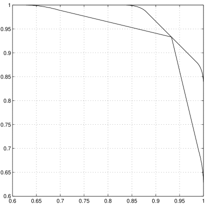
Figure 8: The inner curve bounds the region of $(p_{0|0}^{(1)},p_{1|1}^{(1)})$ attained by LOCC measurement on states $\tau_{0,1}$, and the outer curve bounds the region attained by PPT-preserving measurements (from Fig. 5).

References

- [1] B.M. Terhal, D.P. DiVincenzo, and D.W. Leung, “Hiding bits in Bell states,” Submitted to Phys. Rev. Lett., arXive eprint quant-ph/0011042.
- [2] J.S. Bell, “On the Einstein-Podolsky-Rosen paradox,” Physics, vol. 1, pp. 195–200, 1964.
- [3] R. Cleve and H. Buhrman, “Substituting quantum entanglement for communication,” Phys. Rev. A, vol. 56, no. 2, pp. 1201–1204, 1997.
- [4] A. Peres and W.K. Wootters, “Optimal detection of quantum information,” Phys. Rev. Lett., vol. 66, pp. 1119–1122, 1991.
- [5] C.H. Bennett, D.P. DiVincenzo, C.A. Fuchs, T. Mor, E.M. Rains, P.W. Shor, J.A. Smolin, and W.K. Wootters, “Quantum nonlocality without entanglement,” Phys. Rev. A, vol. 59, pp. 1070–1091, 1999.
- [6] J. Walgate, A.J. Short, L. Hardy, and V. Vedral, “Local distinguishability of multipartite orthogonal quantum states,” Phys. Rev. Lett., vol. 85, pp. 4972–4975, 2000.
- [7] C.H. Bennett, D.P. DiVincenzo, J.A. Smolin, and W.K. Wootters, “Mixed state entanglement and quantum error correction,” Phys. Rev. A, vol. 54, pp. 3824–3851, 1996.
- [8] D. Gottesman, Stabilizer Codes and Quantum Error Correction, Ph.D. thesis, CalTech, 1997.
- [9] J.I. Cirac, W. Dür, B. Kraus, and M. Lewenstein, “Entangling operations and their implementation using a small amount of entanglement,” Phys. Rev. Lett., vol. 86, pp. 544–547, 2001.
- [10] M.-D. Choi, “Completely positive linear maps on complex matrices,” Linear Algebra and Its Applications, vol. 10, pp. 285–290, 1975.
- [11] M.A. Nielsen and I.L. Chuang, Quantum computation and quantum information, Cambridge University Press, Cambridge, U.K., 2000.
- [12] B.W. Schumacher, “Sending entanglement through noisy quantum channels,” Phys. Rev. A, vol. 54, pp. 2614, 1996.
- [13] A. Peres, “Separability criterion for density matrices,” Phys. Rev. Lett., vol. 77, pp. 1413–1415, 1996.
- [14] M. Horodecki, P. Horodecki, and R. Horodecki, “Separability of mixed states: necessary and sufficient conditions,” Physics Letters A, vol. 223, pp. 1–8, 1996.
- [15] E.M. Rains, “Entanglement purification via separable superoperators,” 1997, arXive eprint quant-ph/9707002.
- [16] A. Peres, Quantum Theory: Concepts and Methods, Kluwer Academic Publishers, 1993.
- [17] R.F. Werner, “Quantum states with Einstein-Podolsky-Rosen correlations admitting a hidden-variable model,” Phys. Rev. A, vol. 40, pp. 4277–4281, 1989.
- [18] D.P. DiVincenzo, P.W. Shor, J.A. Smolin, B.M. Terhal, and A.V. Thapliyal, “Evidence for bound entangled states with negative partial transpose,” Phys. Rev. A, vol. 61, pp. 062312, 2000.
- [19] W. Dür, J.I. Cirac, M. Lewenstein, and D. Bruss, “Distillability and partial transposition in bipartite systems,” Phys. Rev. A, vol. 61, pp. 062313, 2000.
- [20] K.G.H. Vollbrecht and R.F. Werner, “Entanglement measures under symmetry,” arXive eprint quant-ph/0010095.
- [21] E. Knill, “Approximating quantum circuits,” arXive eprint quant-ph/9508006.
- [22] A.R. Calderbank, E.M. Rains, P.W. Shor, and N.J.A. Sloane, “Quantum error correction via codes over GF(4),” IEEE Trans. on Inf. Theory, vol. 44, no. 4, pp. 1369–1387, 1998.
- [23] M. Jerrum and A. Sinclair, The Markov Chain Monte Carlo Method: An Approach to Approximate Counting and Integration, PWS Publishing, Boston, 1996, Available at homepage of A. Sinclair.
- [24] P. Diaconis and L. Saloff-Coste, “Comparison techniques for random walk on finite groups,” The Annals of Probability, vol. 21, pp. 2131–2156, 1993.
- [25] T.M. Cover and J.A. Thomas, Elements of Information Theory, Wiley, 1991.
- [26] A.S. Holevo, “The capacity of quantum channel with general signal states,” IEEE Trans. on Inf. Theory, vol. 44, pp. 269, 1998.
- [27] W.K. Wootters, “Entanglement of formation of an arbitrary state of two qubits,” Phys. Rev. Lett., vol. 80, pp. 2245, 1998.
- [28] J. Kilian, Uses of Randomness in Algorithms and Protocols, MIT Press, Cambridge, USA, 1989.
- [29] D. Mayers, “Unconditionally secure quantum bit commitment is impossible,” Phys. Rev. Lett., vol. 78, pp. 3414–17, 1997.
- [30] H.-K. Lo and H.F. Chau, “Is quantum bit commitment really possible?,” Phys. Rev. Lett., vol. 78, pp. 3410–13, 1997.
- [31] H.-K. Lo and H.F. Chau, “Unconditional security of quantum key distribution over arbitrarily long distances,” Science, vol. 283, no. 5410, pp. 2050–2056, 1999.
- [32] K. Mattle, H. Weinfurter, P.G. Kwiat, and A. Zeilinger, “Dense coding in experimental quantum communication,” Phys. Rev. Lett., vol. 76, pp. 4656–4659, 1996.
- [33] S. Takeuchi, J. Kim, Y. Yamamoto, and H.H. Hogue, “Development of a high-quantum-efficiency single-photon counting system,” Appl. Phys. Lett., vol. 74, pp. 1063–1065, 1999.
- [34] E. Knill, R. Laflamme, and G. Milburn, “A scheme for efficient quantum computation with linear optics,” Nature, vol. 409, pp. 46–52, 2001.
- [35] E.M. Rains, “Bound on distillable entanglement,” Phys. Rev. A, vol. 60, pp. 179–184, 1999, erratum: Phys. Rev. A, vol. 63, 019902, 2001.
- [36] E.M. Rains, “Rigorous treatment of distillable entanglement,” Phys. Rev. A, vol. 60, pp. 173–178, 1999.
- [37] T. Eggeling and R.F. Werner, “Separability properties of tripartite states with UUU-symmetry,” arXive eprint quant-ph/0010096.