Theory of Pseudomodes in Quantum Optical Processes

Abstract

This paper deals with non-Markovian behaviour in atomic systems coupled to a structured reservoir of quantum EM field modes, with particular relevance to atoms interacting with the field in high Q cavities or photonic band gap materials. In cases such as the former, we show that the pseudo mode theory for single quantum reservoir excitations can be obtained by applying the Fano diagonalisation method to a system in which the atomic transitions are coupled to a discrete set of (cavity) quasimodes, which in turn are coupled to a continuum set of (external) quasimodes with slowly varying coupling constants and continuum mode density. Each pseudomode can be identified with a discrete quasimode, which gives structure to the actual reservoir of true modes via the expressions for the equivalent atom-true mode coupling constants. The quasimode theory enables cases of multiple excitation of the reservoir to now be treated via Markovian master equations for the atom-discrete quasimode system. Applications of the theory to one, two and many discrete quasimodes are made. For a simple photonic band gap model, where the reservoir structure is associated with the true mode density rather than the coupling constants, the single quantum excitation case appears to be equivalent to a case with two discrete quasimodes.

I Introduction

The quantum behaviour of a small system coupled to a large one has been the subject of many studies since quantum theory was first formulated. The small system is usually of primary interest and generally microscopic (atom, nucleus, molecule or small collections of these) but currently systems of a more macroscopic nature (Bose condensate, superconductor, quantum computer) are being studied. The large system is invariably macroscopic in nature (free space or universe modes of the EM field, lattice modes in a solid, collider atoms in a gas) and is of less interest in its own right, being primarily of relevance as a reservoir or bath affecting the small system in terms of relaxation and noise processes. The large system is often a model for the entire external environment surrounding the small system. Changes in the small system states (described in terms of its density operator) can be divided into two sorts—effects on the state populations (energy loss or gain) or effects on the state coherences (decoherence or induced coherence). Equivalently, quantum information (described via the von Neumann entropy) would be lost or gained due to the interaction with the environment, and its loss is generally associated with decoherence. Interestingly, as the small system becomes larger or occupies states that are more classical the time scale for decoherence can become much smaller than that for energy loss. This is of special interest in quantum information processing [1, 2, 3] where the small system is a collection of qbits making up a quantum computer weakly coupled to the outside world, or in measurement theory [4, 5, 6, 7], where the small system is a micro system being measured coupled to an apparatus (or pointer) that registers the results. For quantum computers it is desirable that decoherence is negligible during the overall computation time [8] (otherwise error correction methods have to be incorporated, and this is costly in terms of processing time), whereas in measurement theory environment induced decoherence [4, 9] is responsible for the density operator becoming diagonal in the pointer basis (otherwise a macroscopic superposition of pointer readings would result).

A standard method for describing the reservoir effects on the small system is based on the Born-Markoff master equation for the system density operator [10, 11, 12, 13]. This depends on the correlation time for the reservoir (as determined from the behaviour of two time correlation functions for pairs of reservoir operators involved in the system reservoir interaction) being very short compared to that of the relaxation and noise processes of the system. In general terms, the more slowly varying the coupling constants for this interaction or the density of reservoir states are with reservoir frequencies, the shorter the correlation time will be. For many situations in the fields of quantum optics, NMR, solid state physics the Born-Markoff master equation provided an accurate description of the physics for the system. Elaborations or variants of the method such as quantum state trajectories [14, 15], Fokker-Planck or c-number Langevin equations [10, 16], quantum Langevin equations [10, 11, 13] are also used. Sometimes an apparently non-Markovian problem can be converted to a Markovian one by a more suitable treatment of the internal system interactions (for example, the use of dressed atom states [17, 18] for treating driven atoms in narrow band squeezed vacuum fields [19, 20]).

However, situations are now being studied in which the standard Born-Markoff approach is no longer appropriate, since the reservoir correlation times are too long for the time scales of interest. A structured rather than flat reservoir situation applies [21, 22]. This includes cases where the reservoir coupling constants vary significantly with frequency, such as the interaction of atom(s) or quantum dots with light in high Q cavities [23], including microcavities (see, for example, [24, 25, 26, 27, 28]) and microspheres (see, for example, [29, 30]). Cases such as an atom (or many atoms—super-radiance) interacting with light in photonic band gap materials [21, 31, 32, 33],[34, 35], where the reservoir mode densities that have gaps and non-analytic behaviour near the band gap edges, also occur. Also, quantum feedback situations [36, 37] can involve significant time delays in the feedback circuit, and thus result in non-Markovian dynamics for the system itself. Furthermore, systems with several degrees of freedom, such as in quantum measurements (for example, the Stern-Gerlach experiment) could involve situations where the decoherence times associated with some degrees of freedom (such as the position of the atomic spin) could become so short that the Markoff condition might no longer be valid, and the effects of such non-Markovian relaxation on the decoherence times associated with more important degrees of freedom (atom spin states) would be of interest.

A number of methods for treating non-Markovian processes have been developed. Apart from direct numerical simulations [38], these include the Zwanzig-Nakajima non-Markovian master equation and its extensions [39, 40, 41], the time-convolutionless projection operator master equation [42], Heisenberg equations of motion [33, 43], stochastic wave function methods for non-Markovian processes [44, 45, 46, 47, 48, 49], methods based on the essential states approximation or resolvent operators [21, 32, 50], the pseudo mode approach [51, 52], Fano diagonalisation [53, 12, 54] and the sudden decoherence approximation [55]. Of these methods the last four are easier to apply and give more physical insight into what is happening. However the essential states method is difficult to apply in all but the simplest situations, since the set of coupled amplitude equations becomes unwieldy and it is difficult to solve—as in the case where multiple excitations of the reservoir are involved. The pseudo mode approach is based on the idea of enlarging the system to include part of the reservoir (the pseudo mode—which could be bosonic or fermionic depending on the case) thereby forming a bigger system in which the Markoff approximation now applies when the coupling to the remainder of the reservoir is treated. At present the pseudomode method is also restricted to single reservoir excitation cases. The Fano diagonalisation method relates the causes of non-Markovian effects to various underlying features (such as the presence of bound states for treating atom lasers), and is closely related to the pseudo mode method. The sudden decoherence method enables decoherence effects on time scales short compared to system Bohr periods to be treated simply via ignoring the system Hamiltonian.

This paper deals with the relationship between the current pseudo mode method for single quantum reservoir excitations and the Fano diagonalisation method for situations where the reservoir structure is due to the presence of a discrete, system of (quasi) modes which are coupled to other continuum (quasi) modes. This important case applies to atomic systems coupled to the quantum EM field in high Q resonant cavities, such as microspheres or microcavities. It is shown that the pseudo mode method for single quantum excitations of the structured reservoir can be obtained by applying the Fano diagonalisation method to a system featuring a set of discrete quasi modes [56, 57] together with a set of continuum quasi modes, whose mode density is slowly varying. The structured reservoir of true modes [58, 59] is thus replaced by the quasi modes. The interaction between the discrete and continuum quasi modes is treated in the rotating-wave approximation and assuming slowly varying coupling constants [60, 61]. The atomic system is assumed to be only coupled to the discrete quasi modes. The density of continuum quasi modes is explicitly included in the model. Although the behavior of the atomic system itself is non-Markovian, the enlarged system obtained by combining the discrete quasi modes with the atomic system now exhibits Markovian dynamics. The discrete quasi modes are identified as pseudo modes. The continuum quasi modes are identified as the flat reservoir to which the enlarged Markovian system is coupled. Explicit expressions for the atom-true modes coupling constants are obtained, exhibiting the rapidly varying frequency dependence characteristic of structured reservoirs. At present the treatment is restricted to cases where threshold and band gap effects are unimportant, but may be applicable to two-dimensional photonic band gap materials. However, the problem of treating multiple excitation processes for certain types of structured reservoirs can now be treated via the quasimode theory, since the Markovian master equation for the atom-quasi mode system applies for cases involving multilevel atoms or cases of several excited two-level atoms. Further extensions of the treatment to allow for atomic systems driven by single mode external laser fields are also possible, with the original atomic system being replaced by the dressed atom.

The plan of the paper is as follows. In Section II the key features of pseudo mode theory are outlined. Section III presents the Fano diagonalisation theory for the quasi mode system, with details covered in the Appendices A, B and C. In Section IV specific cases such as one or two discrete quasi modes or where the variation of discrete-continuum coupling constants can be ignored are examined, giving results for the atom-true mode coupling constants and reservoir structure functions in these situations. Section V contains the Markovian master equation for the atom plus discrete quasi modes system. Section VI briefly examines the situation where coupling constants and mode densities are not slowly varying. Conclusions and comments are set out in Section VII.

II Pseudomode Theory

The simplest case to which pseudomode theory [51] can be applied is that of a two-level atom coupled to the modes of the quantum electromagnetic (EM) field—which constitutes the structured reservoir. Only one photon excitation processes will occur. However, the formalism would also apply to any spin 1/2 fermion system coupled to a bath of bosonic oscillators. The Hamiltonian is given in the rotating wave approximation by:

$$\hat{H} = \sum_{\lambda}\hbar\omega_{\lambda}\hat{a}_{\lambda}^{\dagger}\hat{a}_{\lambda}+{\frac{1}{2}}\hbar\omega_{1}\left(\hat{\sigma}^{+}\hat{\sigma}^{-}-\hat{\sigma}^{-}\hat{\sigma}^{+}\right)$$ (2)

$$+\sum_{\lambda}\left(\hbar g_{\lambda}^{\ast}\hat{a}_{\lambda}\hat{\sigma}^{+}+\mbox{h.c.}\right)$$

where $\hat{\sigma}^{+},\hat{\sigma}^{-}$ are the usual atomic spin operators, $\hat{a}_{\lambda}$, $\hat{a}_{\lambda}^{\dagger}$ are the annihilation, creation operators for the mode $\lambda$ of the field, $\omega_{1}$ is the atomic transition frequency, $\omega_{\lambda}$ is the mode frequency and $g_{\lambda}$ are the coupling constants. This system is illustrated in Fig. 1.

To describe a one photon excitation process, the initial condition is the atom excited and no photons present in the field. Hence the initial Schrodinger picture state vector is:

$$|\Psi(0)\rangle=|1\rangle|...0_{\lambda}...\rangle$$ (3)

In the essential states approach the state vector at later time $t$ will be a superposition of the initial state and states with the atom in its lower state and one photon in various modes $\lambda$. With $\tilde{c}_{1},\tilde{c}_{\lambda}$ defining the complex amplitudes for the atomic excited state and the one photon states, the state vector is:

$$|\Psi(t)\rangle=\tilde{c}_{1}(t)\mbox{e}^{-i\omega_{1}t}|1\rangle|...0_{\lambda}...\rangle+\sum_{\lambda}\tilde{c}_{\lambda}(t)\mbox{e}^{-i\omega_{\lambda}t}|0\rangle|...1_{\lambda}...\rangle$$ (4)

Substitution into the time dependent Schrodinger equation leads to the following coupled complex amplitude equations:

$$i\frac{\mbox{d}}{\mbox{d}t}\tilde{c}_{1} = \sum_{\lambda}g_{\lambda}^{\ast}\mbox{e}^{-i\Delta_{\lambda}t}\tilde{c}_{\lambda}$$ (5)

$$i\frac{\mbox{d}}{\mbox{d}t}\tilde{c}_{\lambda} = g_{\lambda}\mbox{e}^{i\Delta_{\lambda}t}\tilde{c}_{1}$$ (6)

where $\Delta_{\lambda}=\omega_{\lambda}-\omega_{1}$ are detunings.

Formally eliminating the amplitudes for the one photon states enables an integro-differential equation for the excited atomic amplitude to be derived. This is:

$$\frac{\mbox{d}}{\mbox{d}t}\tilde{c}_{1}(t)=-\int_{0}^{t}\mbox{d}\tau\tilde{G}(\tau)\tilde{c}_{1}(t-\tau)$$ (7)

and involves a kernel $\tilde{G}$ given by

$$\tilde{G}(\tau) = \sum_{\lambda}|g_{\lambda}|^{2}\mbox{e}^{-i\Delta_{\lambda}\tau}$$ (8)

$$= \int d\omega_{\lambda}\rho(\omega_{\lambda})|g_{\lambda}|^{2}\mbox{e}^{-i\Delta_{\lambda}\tau}$$ (9)

The mode density $\rho(\omega_{\lambda})$ is introduced after replacing the sum over $\lambda$ by an integral over the mode angular frequency $\omega_{\lambda}$.

It is apparent from Eq.(7) that the behaviour of the atomic system only depends on the reservoir structure function $D(\omega_{\lambda})$ for this single quantum excitation case defined by

$$\rho_{\lambda}\left|g_{\lambda}\right|^{2}=\frac{\Omega^{2}}{2\pi}D(\omega_{\lambda})$$ (10)

where a transition strength $\Omega$ is introduced to normalise $D$ so that its integral gives $2\pi$. The transition strength $\Omega$ is given by:

$$\Omega^{2}=\int d\omega_{\lambda}\rho(\omega_{\lambda})|g_{\lambda}|^{2}$$ (11)

The reservoir structure function $D(\omega_{\lambda})$ enables us to describe the various types of reservoir to which the atomic system is coupled. If $D$ is slowly varying as a function of $\omega_{\lambda}$ then the reservoir is ‘flat’, whilst ‘structured’ reservoirs are where $D$ varies more rapidly, as seen in Figure 1. There are of course two factors involved in determining the behaviour of $D$—the mode density $\rho(\omega_{\lambda})$ and the coupling constant via $|g_{\lambda}|^{2}$. Either or both can determine how structured the reservoir is. Photonic band gap materials are characterised by mode densities which are actually zero over the gaps in the allowed mode frequencies, and which have non analytic behaviours near the edges of the band gaps. All mode densities are zero for negative $\omega_{\lambda}$, so threshold effects are possible. In cavity QED situations, such as for microspheres and other high Q cavities, the coupling constant varies significantly near the cavity resonant frequencies, so in these cases it is the coupling constant that gives structure to the reservoir. For the present it will be assumed that (apart from simple poles) $D$ is analytic in the lower half complex $\omega_{\lambda}$ plane, and any other non analytic features can be disregarded. It is recognized of course that this restriction places a limit on the range of applicability of the theory, though it may be possible to extend this range by representing the actual function $D(\omega_{\lambda})$ in an approximate form that satisfies the analyticity requirements. In addition (in order to calculate the contour integrals) it will be assumed that $D$ tends to zero at least as fast as $1/|\omega_{\lambda}|$ as $|\omega_{\lambda}|$ tends to infinity.

Based on the above assumption regarding the reservoir structure function $D$, the kernel $G$ may be evaluated in terms of the poles and residues of $D(\omega_{\lambda})$ in the lower half complex $\omega_{\lambda}$ plane. It is assumed that these simple poles can be enumerated. The poles are located at $z_{1},z_{2},....z_{l}...$ and their residues are $r_{1},r_{2},...r_{l}...$. The pole $z_{l}$ may be expressed in terms of a real angular frequency $\omega_{l}$ and a width factor $\Gamma_{l}$ via $z_{l}=\omega_{l}-i\Gamma_{l}/2$. Contour integration methods show that the sum of the residues equals $i$. The kernel is obtained in the form:

$$\tilde{G}(\tau)=-i\Omega^{2}\sum_{l}r_{l}e^{-i(z_{l}-\omega_{1})\tau}$$ (12)

The integro-differential equation (7) for the excited atomic amplitude involves a convolution integral on the right hand side and may be solved using Laplace transform methods. The atomic behaviour obtained is well known [58, 59] and will not be rederived here. It is found that there are two regimes, depending on the ratio of the transition strength to typical width factors. These are: (a) a strong coupling regime with Non-Markovian atomic dynamics, and occuring when $\Omega\gg\Gamma$ (b) a weak coupling regime with Markovian atomic dynamics, occuring when $\Omega\ll\Gamma$.

The pseudomode approach continues by considering poles of the reservoir structure function $D(\omega_{\lambda})$ in the lower half complex $\omega_{\lambda}$ plane. Each pole will be associated with one pseudomode. Reverting to Schrodinger picture amplitudes via $c_{1}(t)=\tilde{c}_{1}(t)\mbox{e}^{-i\omega_{1}t}$ etc., pseudomode amplitudes associated with each pole of $D$ are introduced as defined by:

$$b_{l}(t)=-i\Omega\sqrt{-ir_{l}}e^{-iz_{l}t}\int_{0}^{t}\mbox{d}t^{\prime}e^{iz_{l}t^{\prime}}c_{1}(t^{\prime})$$ (13)

From the definition of $b_{l}$ and by substituting the form (Eq.(12)) for the kernel $G$ that involves the poles of $D$, it is not difficult to show that the excited atomic amplitude and the pseudo mode amplitudes satisfy the following coupled equations:

$$i\frac{dc_{1}(t)}{dt} = \omega_{1}c_{1}(t)+\sum_{l}{\cal K}_{l}b_{l}(t)$$ (14)

$$i\frac{db_{l}(t)}{dt} = z_{l}b_{l}(t)+{\cal K}_{l}c_{1}(t)$$ (15)

where ${\cal K}_{l}=\Omega\sqrt{-ir_{l}}$ are pseudomode coupling constants. In general, the residues $r_{l}$ are not pure imaginary, so the pseudomode coupling constants are not real.

The important point is that the atom plus pseudomodes system now satisfies Markovian equations (Eq.(15)). With a finite (or countable) set of pseudomodes, the original atom plus structured continuum has now been replaced by a simpler system which still enables an exact description of the atomic behaviour to be obtained. Exact master equations involving the pseudomodes have been derived, and in general the pseudomodes can be coupled (see [51]). There are however, difficulties in cases where the pseudomode coupling constants are not real, which can occur in certain cases where there are several pseudomodes. Apart from the general difficulty associated with situations where (apart from having simple poles) the reservoir structure function $D$ is not analytic in the lower half complex plane, there is also considerable difficulty in extending the above theory to treat cases where multiple excitations of the structured reservoir occur, such as when the two-level atom is replaced by a three-level atom in a cascade configuration with the atom is initially in the topmost state. The problem is that applying the usual essential states approach leads to two (or more) photon states now appearing in the state vector (cf. Eq.(4)), and the resulting coupled amplitude equations (cf. Eq.(6)) do not apear to facilitate the sucessive formal elimination of the one, two, .. photon amplitudes, as is possible in the single photon excitation case treated above. It is therefore not clear how pseudomode amplitudes can be introduced, along the lines of Eq.(13) so the pseudomode method has not yet been generalised from its original formulation to allow for multiple reservoir excitations.

III Fano Diagonalisation for a Quasi Mode System

A Description of the approach

The case of multiple excitation of a structured reservoir involves systems more complex than the two level atom treated above. It will be sufficient for the purpose of linking the pseudomode and Fano diagonalisation methods to consider single multilevel atomic systems, although multiatom systems would also be suitable as both systems could result in multiphoton excitations of the quantum EM field. Accordingly the two level Hamiltonian given as the second term in Eq.(2) is now replaced by the multilevel atomic Hamiltonian:

$$\hat{H}_{A}=\sum_{k}\eta_{k}\hbar\omega_{k}\left(\hat{\sigma}_{k}^{+}\hat{\sigma}_{k}^{-}-\hat{\sigma}_{k}^{-}\hat{\sigma}_{k}^{+}\right)$$ (16)

The index $k$ represents an atomic transition associated with a pair of energy levels ($k\equiv\{u,l\}$) with energy difference $\hbar\omega_{k}$. The quantities $\eta_{k}$ are numbers chosen so that $\hat{H}_{A}$ equals the atomic Hamiltonian, apart from an additive constant energy. For example, in a two level atom $\eta$ $=\frac{1}{2}$ for the single transition, whilst in a three level atom in a V configuration with degenerate upper levels $\eta_{1}$ $=\eta_{2}=\frac{1}{3}$ for the two optical frequency transitions, and $\eta_{3}=0$ for the zero frequency transition. Details are set out in Appendix A. The atomic transition operators are $\hat{\sigma}_{k}^{+}\equiv|u\rangle\langle l|\equiv(\hat{\sigma}_{k}^{-})^{\dagger}$. As the Hamiltonians for other fermionic systems can also be written in the same form as in Eq.(16), the treatment is not just restricted to single multilevel atom systems.

As indicated in Section II, an important pseudo mode situation is where the reservoir structure is due to the presence of a discrete, system of (quasi) modes which are coupled to other continuum (quasi) modes with slowly varying coupling constants. This important case applies to atomic systems coupled to the quantum EM field in high Q resonant cavities, such as microspheres or microcavities. The Fano diagonalisation method is then based around the idea that the structured reservoir of quantum EM field modes can be described in two different ways, which will now be outlined. Figure 2 illustrates these two descriptions, along with that involving pseudo modes.

1 Quasi modes

The first approach is to treat the quantum EM field in terms of a quasi mode description [56, 57]. The quasi modes behave as coupled quantum harmonic oscillators. These are to consist of two types, the first being a set of discrete quasi modes, the second being a set of continuum quasi modes. In a typical structured reservoir situation for the area of cavity QED [60], the quasi modes represent a realistic description of the physical system. The discrete modes would be cavity quasi modes—one for each cavity resonance and appropriate for describing the EM field inside the cavity, the continuum modes would be external quasi modes which are describe the field outside the cavity. The interaction between the discrete and continuum quasi modes will be treated in the rotating-wave approximation assuming slowly varying coupling constants [60, 57, 61]. Rotating-wave approximation couplings between the discrete quasi modes are also included, but couplings between the continuum quasi modes are not included—such couplings can be removed by pre-diagonalisation. For the quasi mode description the field Hamiltonian is given by:

$$\hat{H}_{F} = \sum_{i}\hbar\omega_{i}\hat{a}_{i}^{\dagger}\hat{a}_{i}+\sum_{i\neq j}\hbar v_{ij}\hat{a}_{i}^{\dagger}\hat{a}_{j}$$ (19)

$$+\sum_{i}\int d\Delta\rho_{c}(\Delta)\left[\hbar W_{i}(\Delta)\hat{a}_{i}^{\dagger}\hat{b}(\Delta)+\mbox{h.c.}\right]$$

$$+\int d\Delta\rho_{c}(\Delta)\,\hbar\Delta\hat{b}^{\dagger}(\Delta)\hat{b}(\Delta)$$

where $\hat{a}_{i}$, $\hat{a}_{i}^{\dagger}$ are the annihilation, creation operators for the discrete quasi mode $i$, $\omega_{i}$ is its frequency, $\hat{b}(\Delta),\hat{b}^{\dagger}(\Delta)$ are the annihilation, creation operators for the continuum quasi mode of frequency $\Delta$, the coupling constants between the $i,j$ discrete quasi modes are $v_{ij}$ ($v_{ij}=v_{ji}^{\ast}$), whilst the quantity $W_{i}(\Delta)$ is the coupling constant between the $i$ discrete and $\Delta$ continuum quasi modes. The integrals over the quasi continuum frequency $\Delta$ involve a quasi continuum mode density $\rho_{c}(\Delta)$. Both $W_{i}(\Delta)$ and $\rho_{c}(\Delta)$ are usually slowly varying. The discrete quasi mode annihilation, creation operators satisfy Kronecker delta commutation rules, whilst those for the continuum quasi mode operators satisfy Dirac delta function commutation rules:

$$[\hat{a}_{i},a_{j}^{\dagger}] = \delta_{ij}$$ (20)

$$[\hat{b}(\Delta),\hat{b}^{\dagger}(\Delta^{\prime})] = \delta(\Delta-\Delta^{\prime})/\rho_{c}(\Delta).$$ (21)

The $\rho_{c\text{ }}$factor on the right hand side gives annihilation and creation operators which are dimensionless.

For the quasi mode description the interaction between the atomic system and the quantum EM field will be given in the rotating-wave approximation and only involve coupling to the discrete quasi modes. This would apply for the typical structured reservoir situation for the area of cavity QED in the familiar case where the atoms are located inside the cavity. The energy of an excited atom escapes to the external region in a two step process: first, a photon is created in a discrete (cavity) quasi mode via the atom-discrete quasi mode interaction, then second, this photon is destroyed and a photon is created in a continuum (external) quasi mode via the discrete-continuum quasi mode coupling. For the quasi mode description the atom-field interaction will be given as:

$$\hat{H}_{AF}=\sum_{k}\,\sum_{i}\,\left(\hbar\lambda_{ki}^{\ast}\hat{a}_{i}\hat{\sigma}_{k}^{+}+\mbox{h.c.}\right)$$ (22)

where $\lambda_{ki}$ is the coupling constant for the $k$ atomic transition and the $i$ quasi mode.

2 True modes

The second way of describing the quantum EM field is in terms of its true modes [58, 59]. The true modes behave as uncoupled quantum harmonic oscillators. These modes are also used in cavity QED and are often referred to as “universe modes”. The pseudomode theory presented in Section II is also based on true modes. For frequencies near to the cavity resonances these modes are large inside the cavity and small outside, for frequencies away from resonance the opposite applies. The distinction between true modes and quasi modes is discussed in some detail in recent papers [56, 62] and their detailed forms and features in the specific case of a planar Fabry-Perot cavity are demonstrated in [60] In terms of true modes the field Hamiltonian is now given in the alternative form as:

$$\hat{H}_{F}=\int d\omega\,\rho(\omega)\hbar\omega\hat{A}^{\dagger}(\omega)\hat{A}(\omega)$$ (23)

where $\hat{A}(\omega),$ $\hat{A}^{\dagger}(\omega)$ are the annihilation, creation operators for the continuum true mode of frequency $\omega$. The integrals over the quasi continuum frequency $\omega$ involve the true continuum mode density $\rho(\omega)$, which is not in general the same function as $\rho_{c}(\Delta)$. It is also not necessarily a slowly varying function of $\omega$. The continuum true mode annihilation, creation operators satisfy Dirac delta function commutation rules:

$$[\hat{A}(\omega),\hat{A}^{\dagger}(\omega^{\prime})]=\delta(\omega-\omega^{\prime})/\rho(\omega)$$ (24)

In all these Hamiltonians the coupling constants have dimensions of frequency, whilst the annihilation and creation operators are dimensionless, as are the atomic transition operators.

3 Relating quasi and true modes

As will be demonstrated in Section III B, Fano diagonalisation involves determining the relationship between the true mode annihilation operators $\hat{A}(\omega)$ and the quasi mode annihilation operators $\hat{a}_{i}$ and $\hat{b}(\Delta)$. The $\hat{A}(\omega)$ will be written as a linear combination of the $\hat{a}_{i}$ (sum over $i$) and $\hat{b}(\Delta)$ (integral over $\Delta$)(see Eq.(29) below), which involves the functions $\alpha_{i}(\omega)$ and $\beta(\omega,\Delta)$. This relationship can be inverted to give the $\hat{a}_{i}$ as an integral over $\omega$ of the $\hat{A}(\omega)$ (see Eq.(69) below). This enables the true mode form of the atom-field interaction to be given as:

$$\hat{H}_{AF}=\sum_{k}\sum_{i}\int d\omega\,\rho(\omega)\left(\hbar\lambda_{ki}^{\ast}\alpha_{i}^{\ast}(\omega)\hat{A}(\omega)\hat{\sigma}_{k}^{+}+\mbox{h.c.}\right)$$ (25)

Comparing Eqs.(22) and (25) we see that the atom-true mode coupling constant $g^{k}(\omega)$ (for the $k$ atomic transition and the $\omega$ true mode) is given by the expression:

$$g^{k}(\omega)=\sum_{i}\lambda_{ki}\alpha_{i}(\omega).$$ (26)

This can be a complicated function of $\omega$ in a structured reservoir, as will be seen from the forms obtained for the function $\alpha_{i}(\omega)$ (for example, Eq.(85)). This expression for the atom-true mode coupling constant is one of the key results in our theory, and enables the pseudomode and quasi mode descriptions of decay processes for structured reservoirs to be related. Note that the true mode coupling constant now involves two factors: the atom-quasi mode coupling constant $\lambda_{ki}$ and the function $\alpha_{i}(\omega)$ that arises from the Fano diagonalisation process.

For the situation where only a single atomic transition $k$ is involved, the equivalent reservoir structure function would be given by:

$$D^{k}(\omega)=C\rho(\omega)|g^{k}(\omega)|^{2}$$ (27)

where $C$ is the normalising constant, which for convenience we will set equal to unity as it does not contain any $\omega$ dependence. This expression will be used to compare the results from the quasi mode approach to those of the present single quantum excitation pseudomode theory. As we will see, the true mode density cancels out.

Finally, athough our results are still correct for cases where the quasi mode density $\rho_{c}(\Delta)$ and the coupling constants $W_{i}(\Delta)$ are not restricted to being slowly varying functions of $\Delta$, their utility where this is not the case is somewhat limited. The theory is mainly intended to apply to the important pseudo mode situation where the reservoir structure is actually due to the presence of a discrete, system of quasi modes which are coupled to other continuum quasi modes via slowly varying coupling constants. For example, the quantum EM field in high Q resonant cavities can be accurately described in terms of the quasi mode model which has these features, the discrete quasi modes being the cavity quasi modes (linked to the cavity resonances) with which the atoms inside the cavity interact, and the continuum quasi modes being the external modes.

As pointed out previously, the structured reservoir can be any set of bosonic oscillators, not just the quantum EM field. The above treatment would thus apply more generally, and we would then refer to discrete quasi oscillators, continuum quasi oscillators or true oscillators. The physical basis for a quasi mode description of the reservoir of bosonic oscillators will depend on the particular situation; in general they will be idealised approximate versions of the true modes.

B Diagonalisation of the quasi mode Hamiltonian: dressing the quasi mode operators

1 Basic equations for Fano diagonalisation

We start with a multiple quasi-mode description of the quantum EM field, for which the Hamiltonian is given above as Eq.(19). This Hamiltonian can also be written in terms of the true mode description as in Eq. (23), and the problem is to relate the true mode annihilation operators $\hat{A}(\omega)$ in terms of the quasi mode annihilation operators $\hat{a}_{i}$ and $\hat{b}(\Delta)$. In view of the rotating wave approximation form of the Hamiltonian, the quasi mode creation operators are not involved in the relationship [56]. Fano diagonalisation for the non-rotating wave approximation has been treated for the case of a single mode coupled to a reservoir in Ref.[63, 64]. In making a Fano diagonalization we will follow the lines of Ref.[12] (Section 6.6 on dressed operators), rather than Ref.[54], but note that a new feature here is the presence of the mode-mode coupling term in the Hamiltonian Eq.(19). In addition, we explicitly include the mode densities from the beginning. The physical realisation of the quasi mode model for the EM field really determines the quasi continuum mode density $\rho_{c}(\Delta)$, just as it does the coupling constants $v_{ij},W_{i}(\Delta)$ and $\lambda_{ki}$. It is therefore important to be able to find the $\rho_{c}(\omega)$ dependence of quantities such as the reservoir structure function $D(\omega)$ (as we will see, the final expression (Eq.(65)) for the latter does not involve the true mode density $\rho(\omega)$). It is of course possible to scale all the other quantities to make $\rho=\rho_{c}=1$, and then rescale afterwards to allow for the actual $\rho,\rho_{c}$ that apply for the system of interest, but this would lead to much duplication of the results we present. For completeness, the scaling is set out in Appendix B.

From the form of the true mode Hamiltonian in Eq.(23) and the commutation rules Eq.(24) to be satisfied by the $\hat{A}(\omega)$, it is clear that the true mode annihilation operators are eigenoperators of the quantum field Hamiltonian $\hat{H}_{F}$ and must satisfy:

$$\left[\hat{A}(\omega),\hat{H}_{F}\right]=\hbar\omega\hat{A}(\omega)$$ (28)

In general, the true mode annihilation operators $\hat{A}(\omega)$ can be expressed as linear combinations of the quasi mode annihilation operators $\hat{a}_{i}$ and $\hat{b}(\Delta)$ in the form ([57, 56]):

$$\hat{A}(\omega)=\sum_{i}\alpha_{i}(\omega)\hat{a}_{i}+\int\,d\Delta\rho_{c}(\Delta)\beta(\omega,\Delta)\hat{b}(\Delta),$$ (29)

where $\alpha_{i}(\omega)$ and $\beta(\omega,\Delta)$ are functions to be determined, and which are dimensionless. This form for $\hat{A}(\omega)$ is then substituted into Eq.(28) and the commutator evaluated using the quasi mode form Eq.(19) for $\hat{H}_{F}$ and the commutation rules in Eq.(21). The coefficients of the the operators $\hat{a}_{i}$ and $\hat{b}(\Delta)$ on both sides of Eq.(28) are then equated, giving a set of coupled equations for the $\alpha_{i}(\omega)$ and $\beta(\omega,\Delta)$. These are:

$$(\omega_{i}-\omega)\alpha_{i}(\omega)+\sum_{j\neq i}v_{ji}\alpha_{j}(\omega)+\int\,d\Delta\rho_{c}(\Delta)\beta(\omega,\Delta)W_{i}^{\ast}(\Delta) = 0$$ (30)

$$(\Delta-\omega)\beta(\omega,\Delta)+\sum_{i}W_{i}(\Delta)\alpha_{i}(\omega) = 0$$ (31)

To solve Eqs.(30), (31) for the unknown $\alpha_{i}(\omega)$ and $\beta(\omega,\Delta)$ we first solve for $\beta$ in terms of the $\alpha_{i}$. This gives:

$$\beta(\omega,\Delta)=\left[\frac{{\cal P}}{\omega-\Delta}+z(\omega)\delta(\omega-\Delta)\right]\sum_{j}W_{j}(\Delta)\alpha_{j}(\omega),$$ (32)

where $z(\omega)$ is a dimensionless function yet to be determined. This expression is then substituted into Eq.(30) to obtain a set of linear homogeneous equations for the $\alpha_{i}(\omega)$ in the form:

$$(\omega_{i}-\omega)\alpha_{i}(\omega)+\sum_{j\neq i}v_{ji}\alpha_{j}(\omega)+\sum_{j}F_{ij}\alpha_{j}(\omega)+\sum_{j}W_{i}^{\ast}(\omega)W_{j}(\omega)\rho_{c}(\omega)z(\omega)\alpha_{j}(\omega)=0.$$ (33)

In these equations, a frequency shift matrix $F_{ij}(\omega)$ appears, which involves a principal integral of products of the discrete-continuum quasi mode coupling constants together with the quasi continuum mode density. This is defined by:

$$F_{ij}(\omega)={\cal P}\int d\Delta\rho_{c}(\Delta)\frac{W_{i}^{\ast}(\Delta)W_{j}(\Delta)}{\omega-\Delta}$$ (34)

and satisfies the Hermiticity condition $F_{ji}=F_{ij}^{\ast}.$

Equation (33) can be written in the matrix form

$${\bf m}\mathchoice{{\hbox{\boldmath$\displaystyle\alpha$}}}{{\hbox{\boldmath$\textstyle\alpha$}}}{{\hbox{\boldmath$\scriptstyle\alpha$}}}{{\hbox{\boldmath$\scriptscriptstyle\alpha$}}}=0$$ (35)

where the column matrix $\mathchoice{{\hbox{\boldmath$\displaystyle\alpha$}}}{{\hbox{\boldmath$\textstyle\alpha$}}}{{\hbox{\boldmath$\scriptstyle\alpha$}}}{{\hbox{\boldmath$\scriptscriptstyle\alpha$}}}\equiv\{\alpha_{1}(\omega),\alpha_{2}(\omega),\alpha_{3}(\omega),...\}^{\top}$ and the square matrix ${\bf m}$ is given by:

$${\bf m}_{ij}(\omega)=(\omega_{i}-\omega)\delta_{ij}+(1-\delta_{ij})v_{ji}+F_{ij}(\omega)+W_{i}^{\ast}(\omega)W_{j}(\omega)\rho_{c}(\omega)z(\omega).$$ (36)

2 Solution of equations for amplitudes $\alpha_{i}(\omega)$ and $\beta(\omega,\Delta)$

The approach used to solve these equations is as follows. It is clear that Eq.(35) can give an (unnormalized) solution for $\textstyle\alpha$ in terms of the function $\rho_{c}(\omega)z(\omega)$. We can now use Eq.(35) itself to obtain the expression for $\rho_{c}(\omega)z(\omega)$, subject to the assumption that the quantity $\sum_{i}W_{i}(\omega)\alpha_{i}(\omega)$ is non-zero. This assumption will be verified a posteriori from the normalisation condition for the $\alpha_{i}(\omega)$, which will follow (see below) from the requirement that the form for the $\hat{A}(\omega)$ given in Eq.(29), satisfies the commutator relation $[\hat{A}(\omega),\hat{A}^{\dagger}(\omega^{\prime})]=\delta(\omega-\omega^{\prime})/\rho(\omega)$, [Eq.(24)]. This indeed leads to a non-zero expression for $\sum_{i}W_{i}(\omega)\alpha_{i}(\omega)$, (see Eq.(50) below). After finding both $\rho_{c}(\omega)z(\omega)$ and $\sum_{i}W_{i}(\omega)\alpha_{i}(\omega)$ the results can be substituted back into the equations (33). By eliminating the factor $\sum_{i}W_{i}(\omega)\alpha_{i}(\omega)$ from the last term in Eqs.(33), we obtain a set of inhomogeneous linear equations for the $\alpha_{i}(\omega)$, which can then be solved for the $\alpha_{i}(\omega)$ (and hence $\beta(\omega,\Delta)$).

The general expression for $\rho_{c}(\omega)$ $z(\omega)$ can be obtained from the matrix equation (35). With ${\bf E}$ the unit matrix we introduce the square matrix ${\bf\Omega}$, the column matrix ${\bf W}^{{\bf\ast}}$ and the row matrix ${\bf W}^{T}$ via:

$${\bf\Omega}_{ij}(\omega)=\omega_{i}\delta_{ij}+(1-\delta_{ij})v_{ji}+F_{ij}(\omega)$$ (37)

and ${\bf W}^{\ast}(\omega)\equiv$ $\{W_{1}^{\ast}(\omega),W_{2}^{\ast}(\omega),W_{3}^{\ast}(\omega),...\}^{\top}$, ${\bf W}^{T}(\omega)\equiv$ $\{W_{1}(\omega),W_{2}(\omega),W_{3}(\omega),...\}$, and then write Eq.(35) in the form:

$$(-(\omega{\bf E}-{\bf\Omega})+\rho_{c}(\omega)z(\omega){\bf W}^{\ast}{\bf W}^{T})\mathchoice{{\hbox{\boldmath$\displaystyle\alpha$}}}{{\hbox{\boldmath$\textstyle\alpha$}}}{{\hbox{\boldmath$\scriptstyle\alpha$}}}{{\hbox{\boldmath$\scriptscriptstyle\alpha$}}}=0.$$ (38)

Now the matrix ${\bf\Omega}$ is Hermitean and positive definite, having real eigenvalues close to the real and positive $\omega_{i}$. The matrix $\omega{\bf E}-{\bf\Omega}$ can be hence assumed to be invertible, so by multiplying Eq.(38) from the left by ${\bf W}^{T}(\omega{\bf E}-{\bf\Omega})^{-1}$ we see that:

$$(-1+\rho_{c}(\omega)z(\omega)J(\omega)){\bf W}^{T}\mathchoice{{\hbox{\boldmath$\displaystyle\alpha$}}}{{\hbox{\boldmath$\textstyle\alpha$}}}{{\hbox{\boldmath$\scriptstyle\alpha$}}}{{\hbox{\boldmath$\scriptscriptstyle\alpha$}}}=0$$ (39)

where the function $J(\omega)$ is defined by

$$J(\omega)={\bf W}^{T}(\omega{\bf E}-{\bf\Omega})^{-1}{\bf W}^{\ast}.$$ (40)

Now the quantity ${\bf W}^{T}\mathchoice{{\hbox{\boldmath$\displaystyle\alpha$}}}{{\hbox{\boldmath$\textstyle\alpha$}}}{{\hbox{\boldmath$\scriptstyle\alpha$}}}{{\hbox{\boldmath$\scriptscriptstyle\alpha$}}}$ is equal to $\sum_{i}W_{i}(\omega)\alpha_{i}(\omega)$, which is assumed to be non zero for reasons explained above. This means that $(-1+\rho_{c}(\omega)z(\omega)J(\omega))=0$, and this gives for $\rho_{c}(\omega)z(\omega)$ the general result:

$$\rho_{c}(\omega)z(\omega)=\left\{\sum_{ij}W_{i}(\omega)(\omega{\bf E}-{\bf\Omega(}\omega{\bf)})_{ij}^{-1}W_{j}^{\ast}(\omega)\right\}^{-1},$$ (41)

which only involves the various coupling constants and angular frequencies, along with the quasi continuum mode density. In general the $\omega$ dependence of the result for $\rho_{c}(\omega)z(\omega)$ is complicated, since both the coupling constants $W_{i}$ and the matrix ${\bf\Omega}$ (via the matrix $F$) will depend on $\omega$. In some important cases however, their $\omega$ dependence can be ignored.

As indicated previously, Eqs.(33) or (35) only determine the $\alpha_{i}(\omega)$ (and hence $\beta(\omega,\Delta)$) to within an arbitary scaling factor, as can be seen from their linear form. The normalisation of the solutions is fixed by noting that we need $\hat{A}(\omega)$, Eq.(29), to satisfy the commutator relation $[\hat{A}(\omega),\hat{A}^{\dagger}(\omega^{\prime})]=\delta(\omega-\omega^{\prime})/\rho(\omega)$, [Eq.(24)]. This leads to the condition:

$$\sum\alpha_{i}(\omega)\alpha_{i}^{\ast}(\omega^{\prime})+\int d\Delta\rho_{c}(\Delta)\beta(\omega,\Delta)\beta^{\ast}(\omega^{\prime},\Delta)=\delta(\omega-\omega^{\prime})/\rho(\omega).$$ (42)

Then substituting for $\beta(\omega,\Delta)$ from Eq.(32) and using Eq.(34), we find after considerable algebra that

$$\sum\alpha_{i}(\omega)\alpha_{i}^{\ast}(\omega^{\prime})+\delta(\omega-\omega^{\prime})\left(\pi^{2}+|z(\omega)|^{2}\right)\rho_{c}(\omega)\sum_{ij}W_{i}(\omega)W_{j}^{\ast}(\omega)\alpha_{i}(\omega)\alpha_{j}^{\ast}(\omega)$$ (43)

$$+\frac{{\cal P}}{\omega-\omega^{\prime}}\sum_{ij}\alpha_{i}(\omega)\alpha_{j}^{\ast}(\omega^{\prime})\left[F_{ij}^{\ast}(\omega^{\prime})-F_{ji}(\omega)\right.$$ (44)

$$\left.+z^{\ast}(\omega^{\prime})\rho_{c}(\omega^{/})W_{i}(\omega^{\prime})W_{j}^{\ast}(\omega^{\prime})-z(\omega)\rho_{c}(\omega)W_{i}(\omega)W_{j}^{\ast}(\omega)\right] = \delta(\omega-\omega^{\prime})/\rho(\omega).$$ (45)

Note that we have used certain properties of the principal parts and delta functions (see, for example Ref. [12]):

$$\delta(\omega-\Delta)\delta(\omega^{\prime}-\Delta) = \delta(\omega-\omega^{\prime})\delta(\omega-\Delta)=\delta(\omega-\omega^{\prime})\delta(\omega^{\prime}-\Delta)$$ (46)

$$\frac{{\cal P}}{\omega^{\prime}-\Delta}\delta(\omega-\Delta) = \frac{{\cal P}}{\omega^{\prime}-\omega}\delta(\omega-\Delta)$$ (47)

$$\frac{{\cal P}}{\omega-\Delta}\,\cdot\,\frac{{\cal P}}{\omega^{\prime}-\Delta} = \frac{{\cal P}}{\omega-\omega^{\prime}}\left(\frac{{\cal P}}{\omega^{\prime}-\Delta}-\frac{{\cal P}}{\omega-\Delta}\right)+\pi^{2}\delta(\omega-\Delta)\delta(\omega^{\prime}-\Delta)$$ (48)

to obtain the last equation. We then also use

$$\frac{{\cal P}}{\omega-\omega^{\prime}}\,\cdot\,(\omega-\omega^{\prime})=1$$ (49)

along with Eq.(33) to substitute for $\sum_{j}F_{ij}^{\ast}(\omega^{\prime})\alpha_{j}^{\ast}(\omega^{\prime})$ and $\sum_{i}F_{ji}(\omega)\alpha_{i}(\omega)$ and obtain finally:

$$\sum_{ij}W_{i}(\omega)W_{j}^{\ast}(\omega)\alpha_{i}(\omega)\alpha_{j}^{\ast}(\omega)=\left|\sum_{i}W_{i}(\omega)\alpha_{i}(\omega)\right|^{2}=\frac{1}{\rho(\omega)\rho_{c}(\omega)(\pi^{2}+|z(\omega)|^{2})}.$$ (50)

This fixes, albeit with the coefficients $W_{i}(\omega)$, the normalization of the $\alpha_{i}(\omega)$. Note the appearance of both mode densities in the result. Finally, with a suitable choice of the overall phase we can fix the result for the important quantity $\sum_{i}W_{i}(\omega)\alpha_{i}(\omega)$ to be:

$$\sum_{i}W_{i}(\omega)\alpha_{i}(\omega)=\frac{1}{\sqrt{\rho(\omega)\rho_{c}(\omega)}(\pi+iz(\omega))}$$ (51)

Having obtained this result for $\sum_{i}W_{i}(\omega)\alpha_{i}(\omega)$ we then substitute back into the equations (33), eliminating this factor from the last term to give a set of inhomogeneous linear equations for the $\alpha_{i}(\omega)$:

$$(\omega-\omega_{i})\alpha_{i}(\omega)-\sum_{j\neq i}v_{ji}\alpha_{j}(\omega)-\sum_{j}F_{ij}\alpha_{j}(\omega)=\frac{W_{i}^{\ast}(\omega)\rho_{c}(\omega)z(\omega)}{\sqrt{\rho(\omega)\rho_{c}(\omega)}(\pi+iz(\omega))}.$$ (52)

After some algebra, introducing the matrix ${\bf\Omega}(\omega)$ from Eq.(37) and then substituting from Eq.(41) for $(\rho_{c}(\omega)z(\omega))^{-1}$, the last equations can be solved for the $\alpha_{i}(\omega)$, giving the solution in matrix form as:

$$\mathchoice{{\hbox{\boldmath$\displaystyle\alpha$}}}{{\hbox{\boldmath$\textstyle\alpha$}}}{{\hbox{\boldmath$\scriptstyle\alpha$}}}{{\hbox{\boldmath$\scriptscriptstyle\alpha$}}}(\omega){\bf=-}i\sqrt{\frac{\rho_{c}(\omega)}{\rho(\omega)}}\frac{1}{(1-i\pi\rho_{c}(\omega){\bf W}^{T}(\omega)(\omega{\bf E}-{\bf\Omega}(\omega))^{-1}{\bf W}^{\ast}(\omega))}(\omega{\bf E}-{\bf\Omega}(\omega))^{-1}{\bf W}^{\ast}(\omega).$$ (53)

In this result all the terms that in general depend on $\omega$ are explicitly identified. It is also convenient to write the inverse matrix in terms of its determinant and the adjugate matrix via:

$$(\omega{\bf E}-{\bf\Omega}(\omega))^{-1}=(\omega{\bf E}-{\bf\Omega}(\omega))^{ADJ}/|\omega{\bf E}-{\bf\Omega}(\omega)|$$ (54)

and then the solution for $\mathchoice{{\hbox{\boldmath$\displaystyle\alpha$}}}{{\hbox{\boldmath$\textstyle\alpha$}}}{{\hbox{\boldmath$\scriptstyle\alpha$}}}{{\hbox{\boldmath$\scriptscriptstyle\alpha$}}}(\omega)$ becomes:

$$\mathchoice{{\hbox{\boldmath$\displaystyle\alpha$}}}{{\hbox{\boldmath$\textstyle\alpha$}}}{{\hbox{\boldmath$\scriptstyle\alpha$}}}{{\hbox{\boldmath$\scriptscriptstyle\alpha$}}}(\omega) = {\bf-}i\sqrt{\frac{\rho_{c}(\omega)}{\rho(\omega)}}\frac{1}{(|\omega{\bf E}-{\bf\Omega}(\omega)|-i\pi\rho_{c}(\omega){\bf W}^{T}(\omega)(\omega{\bf E}-{\bf\Omega}(\omega))^{ADJ}{\bf W}^{\ast}(\omega))}$$ (56)

$$\times(\omega{\bf E}-{\bf\Omega}(\omega))^{ADJ}{\bf W}^{\ast}(\omega).$$

The result for the expansion coefficient $\beta(\omega,\Delta)$ then follows from Eq.(32) and substituting for $\rho_{c}(\omega)z(\omega)$ from Eq.(41). After some algebra we find that:

$$\beta(\omega,\Delta)=-i\frac{1}{\sqrt{\rho(\omega)\rho_{c}(\omega)}}\frac{[\delta(\omega-\Delta)+\frac{{\cal P}}{\omega-\Delta}\rho_{c}(\omega){\bf W}^{T}(\omega)(\omega{\bf E}-{\bf\Omega}(\omega))^{-1}{\bf W}^{\ast}(\omega)]}{(1-i\pi\rho_{c}(\omega){\bf W}^{T}(\omega)(\omega{\bf E}-{\bf\Omega}(\omega))^{-1}{\bf W}^{\ast}(\omega))}$$ (57)

We see that the solutions for the $\alpha_{i}(\omega)$ and $\beta(\omega,\Delta)$ only involve the various coupling constants and the mode densities.

3 Coupling constants and reservoir structure function

Introducing the column matrix $\mathchoice{{\hbox{\boldmath$\displaystyle\lambda$}}}{{\hbox{\boldmath$\textstyle\lambda$}}}{{\hbox{\boldmath$\scriptstyle\lambda$}}}{{\hbox{\boldmath$\scriptscriptstyle\lambda$}}}_{k}\equiv\{\lambda_{k1},\lambda_{k2},\lambda_{k3},...\}^{\top}$ the expression (26) for the coupling constant $g^{k}(\omega)$ can be written as:

$$g^{k}(\omega) = -i\sqrt{\frac{\rho_{c}(\omega)}{\rho(\omega)}}\frac{1}{(|\omega{\bf E}-{\bf\Omega}(\omega)|-i\pi\rho_{c}(\omega){\bf W}^{T}(\omega)(\omega{\bf E}-{\bf\Omega}(\omega))^{ADJ}{\bf W}^{\ast}(\omega))}$$ (59)

$$\times\mathchoice{{\hbox{\boldmath$\displaystyle\lambda$}}}{{\hbox{\boldmath$\textstyle\lambda$}}}{{\hbox{\boldmath$\scriptstyle\lambda$}}}{{\hbox{\boldmath$\scriptscriptstyle\lambda$}}}_{k}^{T}(\omega{\bf E}-{\bf\Omega}(\omega))^{ADJ}{\bf W}^{\ast}(\omega)$$

$$= -i\sqrt{\frac{\rho_{c}(\omega)}{\rho(\omega)}}\frac{Q_{n-1}^{k}(\omega)}{P_{n}(\omega)}$$ (60)

where the functions $P_{n}(\omega)$ and $Q_{n-1}^{k}(\omega)$ are defined by:

$$P_{n}(\omega) = |\omega{\bf E}-{\bf\Omega}(\omega)|-i\pi\rho_{c}(\omega){\bf W}^{T}(\omega)(\omega{\bf E}-{\bf\Omega}(\omega))^{ADJ}{\bf W}^{\ast}(\omega)$$ (61)

$$= |\omega{\bf E}-{\bf\Omega}(\omega)|-i\pi\rho_{c}(\omega)\sum_{ij}W_{i}(\omega)(\omega{\bf E}-{\bf\Omega}(\omega))_{ij}^{ADJ}W_{j}^{\ast}(\omega)$$ (62)

$$Q_{n-1}^{k}(\omega) = \mathchoice{{\hbox{\boldmath$\displaystyle\lambda$}}}{{\hbox{\boldmath$\textstyle\lambda$}}}{{\hbox{\boldmath$\scriptstyle\lambda$}}}{{\hbox{\boldmath$\scriptscriptstyle\lambda$}}}_{k}^{T}(\omega{\bf E}-{\bf\Omega}(\omega))^{ADJ}{\bf W}^{\ast}(\omega)$$ (63)

$$= \sum_{ij}\lambda_{ki}(\omega{\bf E}-{\bf\Omega}(\omega))_{ij}^{ADJ}W_{j}^{\ast}(\omega).$$ (64)

In the case where the $\omega$ dependence of the quantities $\rho_{c}(\omega),F_{ij}(\omega)$ and $W_{i}(\omega)$ can be ignored, $P_{n}(\omega)$ and $Q_{n-1}(\omega)$ would be polynomials in $\omega$ of degrees $n$ and $n-1$ respectively, as will be seen in Section IV.

The reservoir structure function can then be expressed as ($C=1)$:

$$D^{k}(\omega)=\rho_{c}(\omega)\frac{|Q_{n-1}^{k}(\omega)|^{2}}{|P_{n}(\omega)|^{2}}$$ (65)

where we note the cancellation of the true mode density $\rho(\omega)$ and the proportionality to the quasi continuum mode density $\rho_{c}(\omega)$. The significance of the $\rho(\omega)$ cancellation will be discussed in Section III C. There is however further dependence on the quasi continuum mode density within the function $P_{n}(\omega)$, as can be seen from Eq.(62). The role of this dependence will be discussed in Section IV when we have obtained expressions for the reservoir structure function for specific cases.

To sum up: if we are given the Hamiltonian in the quasi mode form Eq.(19), we can obtain the true mode operators (29) which satisfy the eigenoperator condition Eq.(28). The coefficients $\alpha_{i}(\omega)$ are found by solving ${\bf m}\mathchoice{{\hbox{\boldmath$\displaystyle\alpha$}}}{{\hbox{\boldmath$\textstyle\alpha$}}}{{\hbox{\boldmath$\scriptstyle\alpha$}}}{{\hbox{\boldmath$\scriptscriptstyle\alpha$}}}=0$, Eq. (35); the function $z(\omega)$ occuring in ${\bf m}$ is obtained from Eq.(35) and given by Eq.(41). The solutions for $\alpha_{i}(\omega)$ are scaled in accordance with Eq.(42) and the normalisation for the quantity $\sum_{i}W_{i}(\omega)\alpha_{i}(\omega)$ is given in Eqs.(50), (51). The normalised solutions for $\alpha_{i}(\omega)$ are obtained as Eqs.(53) or (56). The coefficients $\beta(\omega,\Delta)$ are then found from Eq.(32) and the result given in Eq.(57). The true mode coupling constant $g^{k}(\omega)$ and the reservoir structure function $D^{k}(\omega)$ are obtained as Eqs.(60) and (65). These results involve the functions $P_{n}(\omega)$ and $Q_{n-1}^{k}(\omega)$ defined in Eqs.(62) and (64). The results depend on the quasi continuum mode density $\rho_{c}$ as well as on the various coupling constants and angular frequencies. It should be noted that a unique expression has been obtained for $z(\omega)$, and hence for the $\alpha_{i}(\omega)$ and $\beta(\omega,\Delta)$, even though the determinental equation $|{\bf m|=}0$ might appear to give anything up to $n$ solutions, where $n$ is the number of discrete quasi modes. This feature is due to the specific form of the matrix ${\bf m}$ that is involved. The overall process amounts to a diagonalization because the EM field Hamiltonian in the non-diagonal quasi mode form is now replaced by the diagonal true mode form given by Eq.(23).

C Inverse diagonalization: undressing the true mode operators

We can also proceed in the opposite direction from Fano diagonalization: that is, we can also find the quasi mode operators $\hat{a}_{i}$ and $\hat{b}(\Delta)$ in terms of the true mode operators $\hat{A}(\omega)$. In general ([57, 56]) the quasi mode annihilation operators $\hat{a}_{i}$ and $\hat{b}(\Delta)$ can also be expressed as linear combinations of the true mode annihilation operators $\hat{A}(\omega)$ in the form:

$$\hat{a}_{i} = \int d\omega\,\rho(\omega)\gamma_{i}(\omega)\hat{A}(\omega)$$ (66)

$$\hat{b}(\Delta) = \int d\omega\,\rho(\omega)\delta(\Delta,\omega)\hat{A}(\omega)$$ (67)

where the functions $\gamma_{i}(\omega)$ and $\delta(\Delta,\omega)$ have to be determined. These can be obtained in terms of the $\alpha_{i}(\omega)$ and $\beta(\omega,\Delta)$ by evaluating the commutators $[\hat{A}(\omega),\hat{a}_{i}^{\dagger}]$ and $[\hat{A}(\omega),\hat{b}(\Delta)^{\dagger}]$ using the basic commutation rules Eqs.(24), (21). For the first commutator: on substituting for $\hat{A}(\omega)$ from Eq.(29) we obtain $\alpha_{i}(\omega)$, on the other hand, substituting instead for $\hat{a}_{i}$ from Eq.(67) gives $\gamma_{i}^{\ast}(\omega)$, and hence $\alpha_{i}=\gamma_{i}^{\ast}$. Carrying out a similar process for the second commutator gives the result $\beta=\delta^{\ast\text{ }}$and thus:

$$\hat{a}_{i} = \int d\omega\,\rho(\omega)\alpha_{i}^{\ast}(\omega)\hat{A}(\omega)$$ (68)

$$\hat{b}(\Delta) = \int d\omega\,\rho(\omega)\beta^{\ast}(\Delta,\omega)\hat{A}(\omega)$$ (69)

As has been already described in Section III A, the first of these two equations enables us to relate the two descriptions of the atom-field interaction given in Eqs.(22) and (25). Ultimately, the key expression we have obtained in Eq.(26) for the atom-true mode coupling constant rests on this result. As we will see in Section IV, this enables us to relate pseudomodes to the discrete quasi modes.

As a final check of the detailed expressions, in Appendix C we start with the field Hamiltonian in the quasi mode form Eq.(19), then substitute our solutions for $\alpha_{i}(\omega)$ and $\beta(\omega,\Delta)$ into the expressions for $\hat{a}_{i}$ and $\hat{b}(\Delta)$ given in Eqs.(69). On evaluating the result, the Hamiltonian in the true mode form Eq.(23) is obtained—as required for consistency.

It has already been noted in Section III B that the final expression for the reservoir structure function $D^{k}(\omega)$ in terms of quasimode quantities is independent of the true mode density $\rho(\omega)$. Also, we have found no equation that actually gives an expression for $\rho(\omega)$ in terms of the quasi mode quantities, including the continuum quasi mode density $\rho_{c}(\Delta)$ - a somewhat surprising result. The true mode density therefore does not play an important role in the quasimode theory. The reason for this is not that hard to find, however. The theory can be recast with both the $\rho(\omega)$ and $\rho_{c}(\Delta)$ factors incorporated into the various operators and coupling constants. In Appendix B we show that $\rho(\omega)$ and $\rho_{c}(\Delta)$ can be scaled away to unity. For example, from Eqs.(53), (57) and (29) we see that the true mode annihilation operator is proportional to $1/\sqrt{\rho(\omega)}$, the other (operator) factor only depending on quasi mode quantities. Hence (as in Appendix B) we may scale away the $\rho(\omega)$ dependence via the substitution:

$$\hat{A}(\omega)=\frac{\hat{A}^{(s)}(\omega)}{\sqrt{\rho(\omega)}}$$ (70)

where $\hat{A}^{(s)}(\omega)$ is independent of $\rho$. If this substitution is made then the field Hamiltonian is given by:

$$\hat{H}_{F}=\int d\omega\,\hbar\omega\hat{A}^{(s)\dagger}(\omega)\hat{A}^{(s)}(\omega)$$ (71)

without any $\rho(\omega)$ term.

IV Applications

A Case of a single quasi mode

For this case no coupling constant between discrete quasi modes is present and we may easily allow for a non zero shift matrix element $F_{11}$ and for non constant $W_{i}(\Delta)$. Noting that $(\omega{\bf E}-{\bf\Omega}(\omega))^{ADJ}=1$ and $|\omega{\bf E}-{\bf\Omega}(\omega)|=\omega-\omega_{1}-F_{11}(\omega)$, a simple evaluation of Eqs.(41), (53) and (60) gives the following results:

$$\rho_{c}(\omega)z(\omega)=\frac{\omega-\omega_{1}-F_{11}(\omega)}{|W_{1}(\omega)|^{2}}$$ (72)

$$\alpha_{1}(\omega)=-i\sqrt{\frac{\rho_{c}(\omega)}{\rho(\omega)}}\frac{W_{1}(\omega)^{\ast}}{\omega-\omega_{1}-F_{11}(\omega)-i\pi\rho_{c}(\omega)|W_{1}(\omega)|^{2}}.$$ (73)

$\displaystyle g^{k}(\omega)=\lambda_{k1}\alpha_{1}(\omega)=-i\sqrt{\frac{\rho_{c}(\omega)}{\rho(\omega)}}\frac{\lambda_{k1}W_{1}(\omega)^{\ast}}{\omega-\omega_{1}-F_{11}(\omega)-i\pi\rho_{c}(\omega)|W_{1}(\omega)|^{2}}$

In terms of a frequency shift $\Delta\omega_{1}$ and half-width $\frac{\Gamma}{2}$ defined as:

$$\Delta\omega_{1}(\omega)=F_{11}(\omega)$$ (74)

$$\frac{\Gamma(\omega)}{2}=\pi\rho_{c}(\omega)|W_{1}(\omega)|^{2}$$ (75)

the reservoir structure function (see Eq.(27)) for the situation where only a single atomic transition $k$ is involved is then found to be $(C=1)$:

$$D^{k}(\omega)=\frac{|\lambda_{k1}|^{2}\cdot\Gamma(\omega)/2\pi}{(\omega-\omega_{1}-\Delta\omega_{1}(\omega))^{2}+\Gamma(\omega)^{2}/4}$$ (76)

In the situation where the quasi mode density $\rho_{c}(\Delta)$ and the coupling constant $W_{1}(\Delta)$ are slowly varying functions of $\Delta$, these quantities can be approximated as constants in the expressions for the frequency shift and width. The reservoir structure function is then a Lorentzian shape with a single pole in the lower-half plane at $\omega_{1}+\Delta\omega_{1}-i\Gamma/2$ corresponding to a single pseudomode. Thus the single discrete quasi mode is associated with a single pseudomode, whose position $z_{1}$ is given by $\omega_{1}+\Delta\omega_{1}-i\Gamma/2$ in terms of quasi mode quantities.

B Case of zero discrete quasi mode-quasi mode coupling and flat reservoir coupling constants

The theory becomes rather simpler if there is no coupling between the discrete quasi modes, that is:

$$v_{ij}\Rightarrow 0$$ (77)

This could be in fact arranged by pre-diagonalising the part of the Hamiltonian $\hat{H}_{F}$ that only involves the discrete quasi mode operators. Thus we write

$$\sum_{i}\hbar\omega_{i}\hat{a}_{i}^{\dagger}\hat{a}_{i}+\sum_{i\neq j}\hbar v_{ij}\hat{a}_{i}^{\dagger}\hat{a}_{j}$$ (78)

in the form

$$\sum_{i}\hbar\xi_{i}\hat{c}_{i}^{\dagger}\hat{c}_{i}$$ (79)

via the transformation

$$\hat{c}_{i}=\sum_{j}U_{ij}\hat{a}_{j}.$$ (80)

where $U$ is unitary. The last equation can be inverted to give the $\hat{a}_{i}$ in terms of the $\hat{c}_{i}$ and the result substituted in other parts of $\hat{H}_{F}$ (Eq.(19)) and $\hat{H}_{AF}$ (Eq.(22)). The original coupling constants $\lambda_{ki}$ and $W_{i}(\Delta)$ would be replaced by new coupling constants via suitable linear combinations involving the matrix $U$, and these generally would have similar properties (e.g., flatness) as the original ones.

The idea of replacing the structured reservoir of true modes by quasi modes, in which the continuum quasi modes constitute a flat reservoir, implies that the discrete-continuum quasi mode coupling constants $W_{i}(\Delta)$ and the quasi continuum mode density $\rho_{c}(\Delta)$ are slowly varying functions of $\Delta$. This results in the shift matrix $F_{ij}$ elements being small, so it would be appropriate to examine the case where they are ignored, that is:

$$F_{ij}\Longrightarrow 0$$ (81)

with both $\rho_{c}$ and the $W_{i}$ are assumed constant.

For the case $v_{ij}=0,F_{ij}=0,\rho_{c}(\Delta)=\rho_{c}$ and $W_{i}(\Delta)=$ $W_{i}$ (constants) the quantities involved in the inverse of the matrix $\omega{\bf E}-{\bf\Omega}(\omega)$ are:

$$|\omega{\bf E}-{\bf\Omega}(\omega)| = (\omega-\omega_{1})(\omega-\omega_{2})...(\omega-\omega_{n})$$ (82)

$$(\omega{\bf E}-{\bf\Omega}(\omega))_{ij}^{ADJ} = (\omega-\omega_{1})(\omega-\omega_{2})...(\omega-\omega_{i-1})(\omega-\omega_{i+1})...(\omega-\omega_{n})\delta_{ij}.$$ (83)

A straightforward application of Eqs.(41) and (56) leads to the simple results:

$$\rho_{c}z(\omega)=\left\{\sum_{i}\frac{|W_{i}|^{2}}{\omega-\omega_{i}}\right\}^{-1}$$ (84)

$$\alpha_{i}(\omega)=-i\sqrt{\frac{\rho_{c}}{\rho(\omega)}}W_{i}^{\ast}\frac{(\omega-\omega_{1})(\omega-\omega_{2})...(\omega-\omega_{i-1})(\omega-\omega_{i+1})...(\omega-\omega_{n})}{P_{n}(\omega)}$$ (85)

where the function $P_{n}(\omega)$, (which is defined in Eq.(62)) is now a polynomial of degree $n$, whose roots are designated as $\xi_{i}$. It is now given by:

$$P_{n}(\omega) = (\omega-\omega_{1})(\omega-\omega_{2})...(\omega-\omega_{n})$$ (87)

$$-i\pi\rho_{c}\sum_{j}|W_{j}|^{2}(\omega-\omega_{1})...(\omega-\omega_{j-1})(\omega-\omega_{j+1})...(\omega-\omega_{n})$$

$$= (\omega-\xi_{1})(\omega-\xi_{2})...(\omega-\xi_{n}).$$ (88)

For the true mode coupling constants $g^{k}(\omega)$, the general result in Eq.(60) can be applied to give:

$$g^{k}(\omega)=-i\sqrt{\frac{\rho_{c}}{\rho(\omega)}}\frac{Q_{n-1}^{k}(\omega)}{(\omega-\xi_{1})(\omega-\xi_{2})...(\omega-\xi_{n})}$$ (89)

where the function $Q_{n-1}^{k}(\omega)$ (which is defined in Eq.(64)) is now a polynomial of order $n-1$, whose roots are designated as $\theta_{i}$. It is now given by:

$$Q_{n-1}^{k}(\omega) = \sum_{i}\lambda_{ki}W_{i}^{\ast}(\omega-\omega_{1})(\omega-\omega_{2})...(\omega-\omega_{i-1})(\omega-\omega_{i+1})...(\omega-\omega_{n})$$ (90)

$$= S_{k}(\omega-\theta_{1})(\omega-\theta_{2})...(\omega-\theta_{n-1}),$$ (91)

where $S_{k}$ is a strength factor defined as:

$$S_{k}=\sum_{i}\lambda_{ki}W_{i}^{\ast}$$ (92)

The reservoir structure function $D^{k}(\omega)$ (see Eq.(65)) for the $k$ transition is then given by $(C=1)$:

$$D^{k}(\omega)=\rho_{c}|S_{k}|^{2}\frac{|(\omega-\theta_{1})(\omega-\theta_{2})...(\omega-\theta_{n-1})|^{2}}{|(\omega-\xi_{1})(\omega-\xi_{2})...(\omega-\xi_{n})|^{2}}.$$ (93)

Since products of the form $(\omega-\xi)(\omega-\xi^{\ast})$ can be written as $(\omega-\mathop{\rm Re}\xi)^{2}+(\mathop{\rm Im}\xi)^{2}$, the behaviour of the reservoir structure function $D^{k}=$ $\rho(\omega)|g^{k}(\omega)|^{2}$ (see Eq.(27)) as a function of $\omega$ is now seen to be determined by the product of $n$ Lorentzian functions associated with $|P_{n}(\omega)|^{2}$ with the modulus squared of the polynomial of degree $n-1$ given by $|Q_{n-1}^{k}(\omega)|^{2}$. The quasi continuum mode density merely provides an uninteresting multiplicative constant, except insofar as it is involved in expressions for the width and shift factors. In the case where there are $n$ discrete quasi modes, then irrespective of the location of the roots $\xi_{i}$ of the polynomial equation $P_{n}(\omega)=0$, the reservoir structure function $D^{k}(\omega)$ for a single quantum excitation has $n$ poles in the lower half plane, each corresponding to either $\xi_{i}$ or $\xi_{i}^{\ast}$. As there are $n$ roots when $n$ discrete quasimodes are present, we see that each discrete quasi mode corresponds to one of the $n$ pseudomodes, whose position $z_{i\text{ }}$is equal to $\xi_{i}$ or to $\xi_{i}^{\ast}$. Thus, for the case here where the coupling constants and the quasi continuum mode density are independent of frequency, the feature that leads to a pseudomode is the presence of a discrete quasi mode.

C Case of two discrete quasi modes

The results in the previous subsection can be conveniently illustrated for the case of two discrete quasi modes. For simplicity we will again restrict the treatment to the situation where $v_{12}=0,F_{ij}=0,\rho_{c}(\Delta)=\rho_{c}$ and $W_{i}(\Delta)=$ $W_{i}$ (constants), and just consider a two-level atom, so only two coupling constants $\lambda_{1},\lambda_{2}$ are involved. In this case the atom-true mode coupling constant can be obtained from Eq.(89) and is:

$$g(\omega)=-i\sqrt{\frac{\rho_{c}}{\rho(\omega)}}\frac{(\lambda_{1}W_{1}^{\ast}+\lambda_{2}W_{2}^{\ast})(\omega-\omega_{0})}{(\omega-\xi_{1})(\omega-\xi_{2})}$$ (94)

where $\omega_{0}$ and the roots $\xi_{1,2}$ of $P_{2}(\omega)=0$ are given by:

$$\omega_{0}=\frac{\lambda_{2}W_{2}^{\ast}}{(\lambda_{1}W_{1}^{\ast}+\lambda_{2}W_{2}^{\ast})}\omega_{1}+\frac{\lambda_{1}W_{1}^{\ast}}{(\lambda_{1}W_{1}^{\ast}+\lambda_{2}W_{2}^{\ast})}\omega_{2}$$ (95)

and

$$\xi_{1,2} = \frac{1}{2}\{(\omega_{1}+\omega_{2})+i\pi\rho_{c}(|W_{1}|^{2}+|W_{2}|^{2})\}$$ (97)

$$\pm\frac{1}{2}\sqrt{\{(\omega_{1}-\omega_{2})+i\pi\rho_{c}(|W_{1}|^{2}-|W_{2}|^{2})\}^{2}-4\pi^{2}\rho_{c}^{2}|W_{1}|^{2}|W_{2}|^{2}}$$

It will also be useful to introduce widths $\Gamma_{i}$ defined by:

$$\Gamma_{i}=2\pi\rho_{c}|W_{i}|^{2}$$ (98)

and which can be later identified (see Section V) as the discrete quasi mode decay rates (Eq.(131)). These results will be now examined for special subcases.

1 Special subcase: Equal quasi mode frequencies

In this case we choose:

$$\omega_{1}=\omega_{2}=\omega_{C}$$ (99)

and find that:

$$\omega_{0} = \omega_{C}$$ (100)

$$\xi_{1,2} = \omega_{C},\omega_{C}+i\pi\rho_{c}(|W_{1}|^{2}+|W_{2}|^{2})$$ (101)

giving for the atom-true mode coupling constant:

$$g(\omega)=-i\sqrt{\frac{\rho_{c}}{\rho(\omega)}}\frac{(\lambda_{1}W_{1}^{\ast}+\lambda_{2}W_{2}^{\ast})}{\omega-\omega_{c}+i\pi\rho_{c}(|W_{1}|^{2}+|W_{2}|^{2})},$$ (102)

and for the reservoir structure function:

$$D(\omega)=\rho_{c}\frac{|\lambda_{1}W_{1}^{\ast}+\lambda_{2}W_{2}^{\ast}|^{2}}{(\omega-\omega_{c})^{2}+([\Gamma_{1}+\Gamma_{2}]/2)^{2}}$$ (103)

This corresponds to a single pole in the lower half plane for the reservoir structure function (see Eq.(27)) and thus only results in a single pseudomode, albeit for a case of two degenerate discrete quasi modes.

2 Special subcase: Equal quasi mode reservoir coupling constants

In this case we choose:

$$W_{1}=W_{2}=W$$ (104)

and find that:

$$\omega_{0} = \omega_{C}+\Delta\omega_{C}$$ (105)

$$\omega_{C} = \frac{1}{2}(\omega_{1}+\omega_{2})$$ (106)

$$\Delta\omega_{C} = \frac{(\lambda_{1}-\lambda_{2})}{2(\lambda_{1}+\lambda_{2})}(\omega_{2}-\omega_{1})$$ (107)

$$\xi_{1,2} = \frac{1}{2}(\omega_{1}+\omega_{2})+i\pi\rho_{c}|W|^{2}\pm\frac{1}{2}\sqrt[2]{(\omega_{1}-\omega_{2})^{2}-4\pi^{2}\rho_{c}^{2}|W|^{4}}$$ (108)

Here $\omega_{0}$ has been written in terms of the quasi modes centre frequency $\omega_{C}$ and a frequency shift $\Delta\omega_{C}$ depending on the difference between the two atom-discrete quasi modes coupling constants $\lambda_{i}$ and the discrete quasi modes detuning. There are now two regimes depending on the relative size of the discrete quasi modes separation $|\omega_{1}-\omega_{2}|$ compared to the square root of the quasi continuum mode density $\sqrt[2]{\rho_{c}}$ times the reservoir coupling constant $W$. Equivalently, the regimes depend on the relative size of the separation $|\omega_{1}-\omega_{2}|$ compared to the width factor (decay rate) $\Gamma=\Gamma_{1}=\Gamma_{2}=2\pi\rho_{c}|W|^{2}.$

a Regime 1: Large separation $|\omega_{1}-\omega_{2}|>\Gamma$

Adopting the convention that $\omega_{1}<\omega_{2}$ we can write

$$\frac{1}{2}\sqrt{(\omega_{1}-\omega_{2})^{2}-4\pi^{2}\rho_{c}^{2}|W|^{4}}=\frac{1}{2}(\omega_{2}-\omega_{1})-\Delta\omega_{R}$$ (109)

where $\Delta\omega_{R}$ is a reservoir induced frequency shift. The atom-true mode coupling constant now becomes:

$$g(\omega)=-i\sqrt{\frac{\rho_{c}}{\rho(\omega)}}\frac{(\lambda_{1}+\lambda_{2})W^{\ast}(\omega-\omega_{C}-\Delta\omega_{C})}{(\omega-\omega_{2}+\Delta\omega_{R}-i\pi\rho_{c}|W|^{2})(\omega-\omega_{1}-\Delta\omega_{R}-i\pi\rho_{c}|W|^{2})}$$ (110)

and the reservoir structure function is then:

$$D(\omega)=\frac{|\lambda_{1}+\lambda_{2}|^{2}(\Gamma/2\pi)(\omega-\omega_{C}-\Delta\omega_{C})^{2}}{((\omega-\omega_{2}+\Delta\omega_{R})^{2}+\Gamma^{2}/4)((\omega-\omega_{1}-\Delta\omega_{R})^{2}+\Gamma^{2}/4)}$$ (111)

The reservoir structure function $D$ (see Eq.(111)) will be zero at the shifted centre frequency $\omega_{C}+\Delta\omega_{C}$. There are two poles in the lower half plane leading to Lorentzian factors centred at frequencies $\omega_{2}-\Delta\omega_{R}$ and $\omega_{1}+\Delta\omega_{R}$ and which have equal widths $2\pi\rho_{c}|W|^{2}$. We note that the effect of the coupling to the reservoir is to decrease the effective discrete quasi modes separation by $2\Delta\omega_{R}$.

b Regime 2: Small separation $|\omega_{1}-\omega_{2}|<\Gamma$

We now write

$$\frac{1}{2}\sqrt{4\pi^{2}\rho_{c}^{2}|W|^{4}-(\omega_{1}-\omega_{2})^{2}}=\pi\rho_{c}|W|^{2}(1-\Delta f_{\Gamma})$$ (112)

where $\Delta f_{\Gamma}$ is a fractional change in width factors associated with discrete quasi mode separation. The atom-true mode coupling constant now becomes:

$$g(\omega)=-i\sqrt{\frac{\rho_{c}}{\rho(\omega)}}\frac{(\lambda_{1}+\lambda_{2})W^{\ast}(\omega-\omega_{C}-\Delta\omega_{C})}{(\omega-\omega_{C}-2i\pi\rho_{c}|W|^{2}(1-\frac{1}{2}\Delta f_{\Gamma}))(\omega-\omega_{C}-i\pi\rho_{c}|W|^{2}\Delta f_{\Gamma})},$$ (113)

and the reservoir structure function is:

$$D(\omega)=\frac{|\lambda_{1}+\lambda_{2}|^{2}(\Gamma/2\pi)(\omega-\omega_{C}-\Delta\omega_{C})^{2}}{((\omega-\omega_{C})^{2}+\Gamma^{2}(1-\frac{1}{2}\Delta f_{\Gamma})^{2})((\omega-\omega_{C})^{2}+\Gamma^{2}(\frac{1}{2}\Delta f_{\Gamma})^{2})}$$ (114)

The reservoir structure function $D$ (see Eq.(114)) will again be zero at the shifted centre frequency $\omega_{C}+\Delta\omega_{C}$. There are two poles in the lower half plane leading to Lorentzian factors both centred at the same frequency $\omega_{C}$, but which have unequal widths $2\pi\rho_{c}|W|^{2}(1-\frac{1}{2}\Delta f_{\Gamma})$ and $\pi\rho_{c}|W|^{2}\Delta f_{\Gamma}$. If $\Delta f_{\Gamma}\ll 1$ one width is much smaller than the other.

In their work on superradiance in a photonic band gap material Bay et al [65] assume as a model for the mode density a so-called Fano profile of the form:

$$\rho(\omega)=\frac{f(\omega-\omega_{C}-q)^{2}}{((\omega-\omega_{C})^{2}+(\frac{1}{2}\kappa)^{2})((\omega-\omega_{C})^{2}+(\frac{1}{2}\gamma)^{2})}$$ (115)

with the two-level atom coupling constant $g(\omega)$ given by a slowly varying function proportional to $\sqrt{\omega}$. It is interesting to note that the reservoir structure function related to their theory is of the same form as that obtained here from Eq.(114) if the following identifications are made:

$$q \longrightarrow -\Delta\omega_{C}$$ (116)

$$\frac{1}{2}\kappa \rightarrow 2\pi\rho_{c}|W|^{2}(1-\frac{1}{2}\Delta f_{\Gamma})$$ (117)

$$\frac{1}{2}\gamma \rightarrow \pi\rho_{c}|W|^{2}\Delta f_{\Gamma}$$ (118)

For situations such as atomic systems coupled to the field in high Q cavities the physics is different of course, with the resonant behaviour in the reservoir structure function being due to the atom-true mode coupling constants rather than the reservoir mode density (which we assume is slowly varying). Nevertheless, our two discrete quasi mode model—with equal reservoir coupling constants $W$ that are large compared to the discrete quasi modes detuning $|\omega_{1}-\omega_{2}|$—does provide an equivalent physical model for the photonic band gap case that Bay et al treated, the lack of which was commented on in the review by Lambropoulos et al [21].

The band gap case was also treated as a specific example by Garraway [51] in the original pseudomode theory paper. A model for the reservoir structure function was assumed in the form of a difference between two Lorentzians:

$$D(\omega)=w_{1}\frac{\Gamma_{1}}{(\omega-\omega_{C})^{2}+(\frac{1}{2}\Gamma_{1})^{2}}-w_{2}\frac{\Gamma_{2}}{(\omega-\omega_{C})^{2}+(\frac{1}{2}\Gamma_{2})^{2}}$$ (119)

where the weights $w_{1},w_{2}$ satisfy $w_{1}-w_{2}=1$. Again, apart from an overall proportionality constant this same form can be obtained here (see Eq.(114)) for the reservoir structure function $D$ if we choose the atom-discrete quasi mode coupling constants $\lambda_{1},\lambda_{2}$ to be equal (so that the frequency shift $\Delta\omega_{C}$ is zero):

$$\lambda_{1} = \lambda_{2}$$ (120)

$$\Delta\omega_{C} = 0$$ (121)

and where the following identifications are made:

$$\frac{1}{2}\Gamma_{1} \rightarrow 2\pi\rho_{c}|W|^{2}(1-\frac{1}{2}\Delta f_{\Gamma})$$ (122)

$$\frac{1}{2}\Gamma_{2} \rightarrow \pi\rho_{c}|W|^{2}\Delta f_{\Gamma}$$ (123)

$$w_{1} \rightarrow \frac{1-\frac{1}{2}\Delta f_{\Gamma}}{1-\Delta f_{\Gamma}}$$ (124)

$$w_{2} \rightarrow \frac{\frac{1}{2}\Delta f_{\Gamma}}{1-\Delta f_{\Gamma}}.$$ (125)

As will be seen in the Section V the existence of unusual forms of the reservoir structure function (such as the presence of Lorentzians with negative weights) does not rule out Markovian master equations applying to the atom-discrete quasi modes system. Thus, for the situation of single quantum excitation, where the pseudomodes are always equivalent to discrete quasi modes, we can always obtain Markovian master equations for pseudomode-atom system.

V Markovian Master Equation for Atom-Discrete Quasi Modes System

A key idea for treating the behaviour of a small system coupled to a structured reservoir is that although the behavior of the small system itself is non-Markovian, an enlarged system can obtained that exhibits Markovian dynamics—and which includes the small system, whose dynamics can be obtained later. In our example of a multilevel atomic system coupled to the the quantum EM field as a structured reservoir, we can proceed as follows. The overall system of the atom(s) plus quantum EM field is partitioned into a Markovian system consisting of the atom plus the discrete quasi modes and a flat reservoir consisting of the continuum quasi modes. The system Hamiltonian $\hat{H}_{S}$ is:

$$\hat{H}_{S} = \sum_{k}\eta_{k}\hbar\omega_{k}\left(\hat{\sigma}_{k}^{+}\hat{\sigma}_{k}^{-}-\hat{\sigma}_{k}^{-}\hat{\sigma}_{k}^{+}\right)+\sum_{i}\hbar\omega_{i}\hat{a}_{i}^{\dagger}\hat{a}_{i}$$ (127)

$$+\sum_{i\neq j}\hbar v_{ij}\hat{a}_{i}^{\dagger}\hat{a}_{j}+\sum_{k}\sum_{i}\left(\hbar\lambda_{ki}^{\ast}\hat{a}_{i}\hat{\sigma}_{k}^{+}+\mbox{h.c.}\right)$$

whilst the reservoir Hamiltonian $\hat{H}_{R}$ is:

$$\hat{H}_{R}=\int d\Delta\rho_{c}(\Delta)\,\hbar\Delta\hat{b}^{\dagger}(\Delta)\hat{b}(\Delta)$$ (128)

and the system-reservoir interaction Hamiltonian $\hat{H}_{{\rm S-R}}$ is:

$$\hat{H}_{{\rm S-R}}=\sum_{i}\int d\Delta\rho_{c}(\Delta)\left[\hbar W_{i}(\Delta)\hat{a}_{i}^{\dagger}\hat{b}(\Delta)+\mbox{h.c.}\right],$$ (129)

so that the total Hamiltonian is still equal to the sum of $\hat{H}_{A},\hat{H}_{F}$ and $\hat{H}_{AF}$, given in Eqs.(16), (19) and (22). The distinction between the non-Markovian true mode treatment and the Markovian quasi mode approach is depicted in Fig. 2.

It is of course the slowly varying nature of the coupling constants $W_{i}(\Delta)$ and the mode density $\rho_{c}(\Delta)$ which results in a Markovian master equation for the reduced density operator $\,\hat{\rho}$ of the atom-discrete quasi modes system. Rather than derive the master equation for the most general state of the reservoir, we will just consider the simplest case in which the reservoir of continuum quasi modes are all in the vacuum state. Again, the coupling constants $W_{i}$ will be assumed constant so that no shift matrix $F_{ij}$ elements are present. The master equation is derived via standard proceedures (Born and Markoff approximations) [12, 20], which require the evaluation of two-time reservoir correlation functions in which the required reservoir operators are the quantities $\int d\Delta\rho_{c}(\Delta)W_{i}(\Delta)\hat{b}(\Delta)$ and their Hermitian adjoints. To obtain Markovian behaviour we require the quantities $\rho_{c}(\Delta)W_{i}(\Delta)W_{j}^{\ast}(\Delta)$ to be slowly varying with $\Delta$, so that the reservoir correlation time $\tau_{c}$ (inversely proportional to the bandwidth of $\rho_{c}(\Delta)W_{i}(\Delta)W_{j}^{\ast}(\Delta)$) is sufficiently short that the interaction picture density operator hardly changes during $\tau_{c}$.

The standard procedure then yields the master equation in the Lindblad form:

$$\frac{d\hat{\rho}}{dt}=\frac{-i}{\hbar}\left[\hat{H}_{S}\,,\,\hat{\rho}\right]\,+\,\sum_{ij}\pi\rho_{c}W_{i}W_{j}^{\ast}\left\{\left[\hat{a}_{j},\hat{\rho}\hat{a}_{i}^{\dagger}\right]+\left[\hat{a}_{j}\hat{\rho},\hat{a}_{i}^{\dagger}\right]\right\}$$ (130)

Direct couplings between the discrete quasi modes involving the $v_{ij}$ are included in the system Hamiltonian $\hat{H}_{S}$. Radiative processes take place via the atom-discrete quasi modes interaction also included in $\hat{H}_{S}$, though still given as in Eq.(22). The loss of radiative energy to the reservoir is described via the relaxation terms in the master equation. The diagonal terms where $i=j$ describe the relaxation of the $i$ th quasi mode in which the decay rate is proportional to $\rho_{c}|W_{i}|^{2}$. A typical decay rate $\Gamma_{i}$ for the $i$ th discrete quasi mode into the reservoir of continuum quasi modes will be:

$$\Gamma_{i}=2\pi\rho_{c}|W_{i}|^{2}$$ (131)

Note that the off-diagonal terms $i\neq j$ involve pairs of discrete quasi mode operators $\hat{a}_{j}$ and $\hat{a}_{i}^{\dagger}$, so there is also a type of rotating wave approximation interaction taking place via the reservoir between these discrete quasi modes, as well as via direct Hamiltonian coupling involving the $v_{ij}$. The standard criterion for the validity of the Born-Markoff master equation Eq.(130) is that $\Gamma\tau_{c}\ll 1$. Processes involving multiphoton excitation of the reservoir (such as may occur for excited multilevel atoms) can be studied using standard master equation methods, thereby enabling multiple excitation of the structured reservoir to be treated via the quasimode theory.

VI Non Slowly-Varying Mode Densities and/or Coupling Constants

The basic model treated in this paper is that of atomic systems coupled to a set of discrete quasi modes of the EM field, which are in turn coupled to a continuum set of quasi modes. Although expressions for the true mode coupling constant and the reservoir structure function have been obtained for the general case where the quasi mode density $\rho_{c}$ and the coupling constants $W_{i}$ are not necessarily slowly varying functions of $\Delta$ (see Eqs.(60) and (65)), the usefulness of the results where this is not the case is somewhat limited. As indicated in the previous section, the master equation for the atom plus discrete quasi modes system will no longer be Markovian, so the enlargement of the system based on adding the discrete quasi modes to produce a Markovian system fails.

Also, for the non slowly varying $\rho_{c}$ or $W_{i}$ case, we can no longer link each discrete quasi mode to a pseudo mode. That this is the situation may be seen both from the general result for the reservoir structure function (Eq.(65)) or the specific result we have obtained for the case where there is a single discrete quasi mode (Eq.(76)). In the former case, the function $P_{n}(\omega)$ would not be a polynomial of degree $n$, and therefore could have more than $n$ roots, leading to more pseudo modes than discrete quasi modes. In the latter case involving just one discrete quasi mode, even having the mode density $\rho_{c}(\omega)$ (and hence $\Gamma(\omega)$) represented by a single peaked function would result in $D(\omega)$ going from a single peaked function to a triple peaked function, corresponding to three pseudo modes.

However, where $\rho_{c}$ or $W_{i}$ are no longer slowly varying, an examination of the underlying causes for this variation may suggest replacing the present atom plus discrete and continuum quasi mode model by a more elaborate system that better represents the physics of the situation, but with only slowly varying parameters now involved. Fano diagonalisation based on such a more elaborate model could produce the desired link up with the pseudo mode approach and enable a suitable, enlarged system to be identified which has Markovian behaviour, as well as overcoming the problem of treating multiple reservoir excitations. One possible elaboration would be to add a further continuum of quasi modes that are fermionic rather than bosonic.

VII Conclusions

The theory presented above is mainly intended to apply to the important situation where the reservoir structure is actually due to the presence of a discrete system of quasi modes which are coupled to other continuum quasi modes via slowly varying coupling constants. For example, the quantum EM field in high Q resonant cavities can be accurately described in terms of the quasi mode model which has these features, the discrete quasi modes being the cavity quasi modes (linked to the cavity resonances) with which the atoms inside the cavity interact, and the continuum quasi modes being the external modes.

For this situation it has been shown that, for the present case of single quantum excitations, the pseudo mode method for treating atomic systems coupled to a structured reservoir of true quantum EM field modes can be obtained by applying the Fano diagonalisation method to the field described in an equivalent way as a set of discrete quasi modes together with a set of continuum quasi modes, whose mode density is assumed to be slowly varying. The interaction between the discrete and continuum quasi modes is treated in the rotating-wave approximation assuming slowly varying coupling constants, and the atomic system is assumed to be only coupled to the discrete quasi modes. The theory includes the true and continuum quasi mode densities explicitly.

Expressions for the quasi mode operators $\hat{a}_{i}$ and $\hat{b}(\Delta)$ in terms of the true mode operators $\hat{A}(\omega)$ (and vice versa) have been found, and explicit forms for the atom-true mode coupling constants have been obtained and related to the reservoir structure function that applies in pseudomode theory. We have seen that the feature that leads to a pseudomode is the presence of a discrete quasi mode. Each discrete quasi mode corresponds to one of the pseudomodes, whose position $z_{i\text{ }}$in the lower half complex plane is determined from the roots $\xi_{i}$ of a polynomial equation depending on the parameters for the quasi mode system.

Although the behavior of the atom itself is non-Markovian, an enlarged system consisting of the atom plus the discrete quasi modes coupled to a flat reservoir consisting of the continuum quasi modes exhibits Markovian dynamics, and the master equation for this enlarged system has been obtained. Using the quasimode theory, processes involving multiphoton excitation of the structured reservoir (such as may occur for excited multilevel atoms) can now be studied using standard master equation methods applied to the atom-discrete quasi modes system. Furthermore, cases with unusual forms of the reservoir structure function for single quantum excitation (for example, containing Lorentzians with negative weights) still result in Markovian master equations. Since for single quantum excitation the pseudomodes are equivalent to discrete quasi modes, we can now always obtain Markovian master equations for pseudomode-atom systems via our approach.

Although not so useful in such cases, the present theory does lead to general expressions for the true mode coupling constant and the reservoir structure function for single quantum excitation. These expressions are still valid for the general case where the quasi mode density $\rho_{c}$ and the coupling constants $W_{i}$ are no longer slowly varying functions of $\Delta$. However, the master equation for the atom plus discrete quasi modes system will no longer be Markovian, so the enlargement of the system based on adding the discrete quasi modes to produce a Markovian system fails. Also, for the non slowly varying $\rho_{c}$ or $W_{i}$ case, we can no longer link each discrete quasi mode to a pseudo mode—there may be more pseudo modes than discrete quasi modes. In such cases it would be desirable to replace the present quasi mode system by a more elaborate quasi mode system involving only slowly varying quantities, and which better represents the underlying physical causes of the variation in $W_{i}$ and $\rho_{c}$ that occurs in the present model. This may make possible an extension of the Fano diagonalisation approach that still links quasi modes with pseudo modes, and results in a Markovian master equation for the enlarged atom plus quasi mode system. In such an elaborated system, the disadvantage of the present pseudo mode treatment in treating multiple excitations of the structured reservoir could still be removed.

The treatment has been outlined in the case of a multilevel atom coupled to a structured reservoir of quantum EM field modes, but a similar approach would apply for any fermionic system coupled to a structured reservoir of bosonic oscillators. Extensions to fermionic reservoirs should be possible also. At present the treatment is restricted to cases where threshold and band gap effects are unimportant, but may be applicable to two-dimensional photonic band gap materials. Further extensions of the treatment to allow for atomic systems driven by single mode external laser fields are also possible, with the original atomic system being replaced by the dressed atom.

VIII Acknowledgments

The authors are grateful to D. G. Angelakis, J. Wang and A. Imamoglu for helpful discussions. This work was supported by the United Kingdom Engineering and Physical Sciences Research Council. SMB thanks the Royal Society of Edinburgh and the Scottish Executive Education and Lifelong Learning Department for the award of a Support Research Fellowship.

A Atomic Hamiltonian

As an example of writing the atomic Hamiltonian in the form given in Eq.(16), consider a three level atom in a V configuration with upper states$\ |2\rangle,|1\rangle$ and lower state $|0\rangle$, whose energy is chosen for convenience to be zero. The atomic transition operators are $\hat{\sigma}_{2}^{+}\equiv|2\rangle\langle 0|$ and $\ \hat{\sigma}_{1}^{+}\equiv|1\rangle\langle 0|$ for the two optical transitions of frequencies $\omega_{2}$ and $\omega_{1}$, and $\hat{\sigma}_{3}^{+}\equiv|2\rangle\langle 1|$ for the Zeeman transition of frequency $\omega_{2}-\omega_{1}$.

The form given in Eq.(16) is:

$$\hat{H}_{A} = \eta_{1}\hbar\omega_{1}\left(\hat{\sigma}_{1}^{+}\hat{\sigma}_{1}^{-}-\hat{\sigma}_{1}^{-}\hat{\sigma}_{1}^{+}\right)+\eta_{2}\hbar\omega_{2}\left(\hat{\sigma}_{2}^{+}\hat{\sigma}_{2}^{-}-\hat{\sigma}_{2}^{-}\hat{\sigma}_{2}^{+}\right)+\eta_{3}\hbar(\omega_{2}-\omega_{1})\left(\hat{\sigma}_{3}^{+}\hat{\sigma}_{3}^{-}-\hat{\sigma}_{3}^{-}\hat{\sigma}_{3}^{+}\right)$$ (A1)

$$= \eta_{1}\hbar\omega_{1}\left(|1\rangle\langle 1|-|0\rangle\langle 0|\right)+\eta_{2}\hbar\omega_{2}\left(|2\rangle\langle 2|-|0\rangle\langle 0|\right)+\eta_{3}\hbar(\omega_{2}-\omega_{1})\left(|2\rangle\langle 2|-|1\rangle\langle 1|\right).$$ (A2)

This expression may also be written in the form

$$\hat{H}_{A}=\hbar\omega_{1}|1\rangle\langle 1|+\hbar\omega_{2}|2\rangle\langle 2|+\hbar\omega(|0\rangle\langle 0|+|1\rangle\langle 1|+|2\rangle\langle 2|),$$ (A3)

since by equating the coefficients of the three projection operators, we obtain a set of linear equations for the $\eta_{1},\eta_{2},\eta_{3}$ and $\omega$ which are solvable $-$ in fact the solutions are not even unique. These equations are:

$$\eta_{2}\omega_{2}+\eta_{3}(\omega_{2}-\omega_{1}) = \omega_{2}+\omega$$ (A4)

$$\eta_{1}\omega_{1}-\eta_{3}(\omega_{2}-\omega_{1}) = \omega_{1}+\omega$$ (A5)

$$-\eta_{1}\omega_{1}-\eta_{2}\omega_{2} = \omega.$$ (A6)

Adding these equations and then substituting into the first two gives:

$$\omega = -\frac{1}{3}(\omega_{1}+\omega_{2})$$ (A7)

$$+\eta_{3}(\omega_{2}-\omega_{1}) = -\frac{1}{3}\omega_{1}+(\frac{2}{3}-\eta_{2})\omega_{2}$$ (A8)

$$-\eta_{3}(\omega_{2}-\omega_{1}) = (\frac{2}{3}-\eta_{1})\omega_{1}-\frac{1}{3}\omega_{2}.$$ (A9)

The last two equations do not produce a unique solution for $\eta_{1},\eta_{2},\eta_{3}$. We can arbitarily choose $\eta_{3}=0$ for the low frequency transition, and then we find that:

$$\eta_{1} = \frac{1}{3}-\frac{1}{3}\frac{(\omega_{2}-\omega_{1})}{\omega_{1}}$$ (A10)

$$\eta_{2} = \frac{1}{3}+\frac{1}{3}\frac{(\omega_{2}-\omega_{1})}{\omega_{2}}.$$ (A11)

This gives $\eta_{1}$ $=\eta_{2}=\frac{1}{3}$ for two degenerate optical frequency transitions.

Comparing the two expressions for $\hat{H}_{A}$ in Eqs.(A2), (A3), where $\eta_{1},\eta_{2}$ are given by Eq.(A11) (with $\eta_{3}$ set to zero) and $\omega$ by Eq.(A7), we see that Eq.(A3) gives the atomic energy apart from the constant term $-\frac{1}{3}\hbar(\omega_{1}+\omega_{2})$.

B Scaling for Mode Densities $\rho(\omega),\rho_{c}(\Delta)$ Equal to Unity

The equations presented in the first part of Section III are based on true and quasi continuum mode densities that are not necessarily equal to unity. To compare our expressions with those in the Ref.[12], we now set out the scalings needed for the various quantities to give the Hamiltonians equivalent to $\hat{H}_{F}$ and $\hat{H}_{AF}$ in either true or quasi mode forms (Eqs.(23), (19), (25) and (22)) in which the mode densities $\rho$ and $\rho_{c}$ are made equal to unity. The creation and anihilation operators are no longer dimensionless, the coupling constants and angular frequencies do not have dimensions of frequency and the expansion coefficients are not dimensionless. The scaled quantities appearing in the Hamiltonians or relationships between annihilation operators will be denoted with a superscript ^(s).

The following replacements made to the annihilation and creation operators:

$$\sqrt{\rho_{c}(\Delta)}\hat{b}(\Delta) \rightarrow \hat{b}^{(s)}(\Delta)$$ (B1)

$$\sqrt{\rho_{c}(\Delta)}\hat{b}^{\dagger}(\Delta) \rightarrow \hat{b}^{(s)\dagger}(\Delta)$$ (B2)

$$\sqrt{\rho(\omega)}\hat{A}(\omega) \rightarrow \hat{A}^{(s)}(\omega)$$ (B3)

$$\sqrt{\rho(\omega)}\hat{A}^{\dagger}(\omega) \rightarrow \hat{A}^{(s)\dagger}(\omega),$$ (B4)

to the coupling constants:

$$\sqrt{\rho_{c}(\Delta)}W_{i}(\Delta)\rightarrow W_{i}^{(s)}(\Delta)$$ (B5)

and to the expansion coefficients:

$$\sqrt{\rho(\omega)}\alpha_{i}(\omega) \rightarrow \alpha_{i}(\omega)^{(s)}$$ (B6)

$$\sqrt{\rho_{c}(\Delta)\rho(\omega)}\beta(\omega,\Delta) \rightarrow \beta^{(s)}(\omega,\Delta)$$ (B7)

will give the Hamiltonians equivalent to $\hat{H}_{F}$ and $\hat{H}_{AF}$ in either true or quasi mode forms (Eqs.(23),(19),(25) and (22)) in which the mode densities are put equal to one. In addition the modified forms of the relationships between true and quasi mode annihilation operators (Eqs.(29) and (69)) can be obtained in which $\rho$ and $\rho_{c}$ are made equal to unity, as can the revised forms of the commutation rules. The latter are:

$$[\hat{b}^{(s)}(\Delta),\hat{b}^{(s)\dagger}(\Delta^{\prime})] = \delta(\Delta-\Delta^{\prime})$$ (B8)

$$[\hat{A}^{(s)}(\omega),\hat{A}^{(s)\dagger}(\omega^{\prime})] = \delta(\omega-\omega^{\prime}).$$ (B9)

In addition the various equations for the $F_{ij}(\omega),\alpha_{i}(\omega),\beta(\omega,\Delta),z(\omega),g^{k}(\omega),D^{k}(\omega)$ now apply with $\rho$ and $\rho_{c}$ put equal to unity. It should be noted that the quantities $\hat{a}_{i},\omega_{i},v_{ij},\Delta,\omega$ are not replaced, nor are any of the atomic quantities $\hat{H}_{A},\eta_{k},\omega_{k},\hat{\sigma}_{k}^{+},\hat{\sigma}_{k}^{-}$ or $\lambda_{ki}$.

C The Hamiltonian $H_{F}$ in Diagonalised Form

We show by starting with the field Hamiltonian in the quasi mode form Eq.(19), substituting the solutions for $\alpha_{i}(\omega)$ and $\beta(\omega,\Delta)$ into the expressions for $\hat{a}_{i}$ and $\hat{b}(\Delta)$ given in Eqs.(69) and then evaluating the result, that the Hamiltonian in the true mode form Eq.(23) is obtained. The symmetry conditions $F_{ij}=F_{ji}^{\ast}$ and $\nu_{ij}=\nu_{ji}^{\ast}$ are used throughout.

Using the expressions for $\hat{a}_{i}$ and $\hat{b}(\Delta)$ given in Eqs.(69) the Hamiltonian in the quasi mode form Eq.(19) is then given by:

$$\hat{H}_{F}=\hbar\int d\omega\rho(\omega)\,\int d\omega^{/}\rho(\omega^{/})\hat{A}^{\dagger}(\omega)\hat{A}(\omega^{/})I(\omega,\omega^{/})$$ (C1)

where the function $I(\omega,\omega^{/})$ is:

$$I(\omega,\omega^{/}) = \sum_{i}\omega_{i}\alpha_{i}(\omega)\alpha_{i}^{\ast}(\omega^{/})+\int d\Delta\rho_{c}(\Delta)\Delta\beta(\Delta,\omega)\beta^{\ast}(\Delta,\omega^{/})$$ (C4)

$$+\sum_{ij(i\neq j)}\nu_{ij}\alpha_{i}(\omega)\alpha_{j}^{\ast}(\omega^{/})+\sum_{i}\int d\Delta\rho_{c}(\Delta)W_{i}(\Delta)\alpha_{i}(\omega)\beta^{\ast}(\Delta,\omega^{/})$$

$$+\sum_{i}\int d\Delta\rho_{c}(\Delta)W_{i}^{\ast}(\Delta)\alpha_{i}^{\ast}(\omega^{/})\beta(\Delta,\omega)$$

Substituting for $\beta(\omega,\Delta)$ in terms of the $\alpha_{i}(\omega)$ from Eq.(32), using the expression (34) for $F_{ij}$ and then Eq.(33) for the $\alpha_{i}(\omega)$ we get for certain contributions within the last two terms in Eq.(C4):

$$\int d\Delta\rho_{c}(\Delta)W_{i}(\Delta)\beta^{\ast}(\Delta,\omega^{/}) = -(\omega_{i}-\omega^{/})\alpha_{i}^{\ast}(\omega^{/})-\sum_{j(j\neq i)}\nu_{ji}^{\ast}\alpha_{j}^{\ast}(\omega^{/})$$ (C5)

$$\int d\Delta\rho_{c}(\Delta)W_{i}^{\ast}(\Delta)\beta(\Delta,\omega) = -(\omega_{i}-\omega)\alpha_{i}(\omega)-\sum_{j(j\neq i)}\nu_{ji}\alpha_{j}(\omega)$$ (C6)

leading to

$$\sum_{i}\int d\Delta\rho_{c}(\Delta)W_{i}(\Delta)\alpha_{i}(\omega)\beta^{\ast}(\Delta,\omega^{/}) = -\sum_{i}(\omega_{i}-\omega^{/})\alpha_{i}(\omega)\alpha_{i}^{\ast}(\omega^{/})-\sum_{ij(j\neq i)}\nu_{ji}^{\ast}\alpha_{i}(\omega)\alpha_{j}^{\ast}(\omega^{/})$$ (C7)

$$\sum_{i}\int d\Delta\rho_{c}(\Delta)W_{i}^{\ast}(\Delta)\alpha_{i}^{\ast}(\omega^{/})\beta(\Delta,\omega) = -\sum_{i}(\omega_{i}-\omega)\alpha_{i}(\omega)\alpha_{i}^{\ast}(\omega^{/})-\sum_{ij(j\neq i)}\nu_{ji}\alpha_{j}(\omega)\alpha_{i}^{\ast}(\omega^{/})$$ (C8)

In the second term of Eq.(C4) substitution for $\beta(\omega,\Delta)$ and $\beta^{\ast}(\omega^{/},\Delta)$ in terms of the $\alpha_{i}(\omega)$ and $\alpha_{j}^{\ast}(\omega^{/})$from Eq.(32) and then using the Eqs.(48) for manipulating principal integrals and delta functions leads to:

$$\int d\Delta\rho_{c}(\Delta)\Delta\beta(\Delta,\omega)\beta^{\ast}(\Delta,\omega^{/}) = \sum_{ij}\{[\int d\Delta\rho_{c}(\Delta)\times$$ (C14)

$$\times\Delta\frac{{\cal P}}{\omega^{/}-\omega}\left(\frac{{\cal P}}{\omega-\Delta}-\frac{{\cal P}}{\omega^{/}-\Delta}\right)W_{i}(\Delta)\alpha_{i}(\omega)W_{j}^{\ast}(\Delta)\alpha_{j}^{\ast}(\omega^{/})]$$

$$+\pi^{2}\delta(\omega-\omega^{/})\rho_{c}(\omega)\omega W_{i}(\omega)\alpha_{i}(\omega)W_{j}^{\ast}(\omega)\alpha_{j}^{\ast}(\omega)$$

$$+\omega^{/}\frac{{\cal P}}{\omega-\omega^{/}}\rho_{c}(\omega^{/})z^{\ast}(\omega^{/})W_{i}(\omega^{/})\alpha_{i}(\omega)W_{j}^{\ast}(\omega^{/})\alpha_{j}^{\ast}(\omega^{/})$$

$$+\omega\frac{{\cal P}}{\omega^{/}-\omega}\rho_{c}(\omega)z(\omega)W_{i}(\omega)\alpha_{i}(\omega)W_{j}^{\ast}(\omega)\alpha_{j}^{\ast}(\omega^{/})$$

$$+\omega\delta(\omega-\omega^{/})\rho_{c}(\omega)z(\omega)z^{\ast}(\omega)W_{i}(\omega)\alpha_{i}(\omega)W_{j}^{\ast}(\omega)\alpha_{j}^{\ast}(\omega)\}$$

Then using Eq.(49) we show that:

$$\Delta\left(\frac{{\cal P}}{\omega-\Delta}-\frac{{\cal P}}{\omega^{/}-\Delta}\right)=\left(\omega\frac{{\cal P}}{\omega-\Delta}-\omega^{/}\frac{{\cal P}}{\omega^{/}-\Delta}\right)$$ (C15)

and following the introduction of the $F_{ij}$ from Eq.(34) we get:

$$\int d\Delta\rho_{c}(\Delta)\Delta\beta(\Delta,\omega)\beta^{\ast}(\Delta,\omega^{/}) = \sum_{ij}\{\omega\frac{{\cal P}}{\omega^{/}-\omega}F_{ji}(\omega)\alpha_{i}(\omega)\alpha_{j}^{\ast}(\omega^{/})$$ (C20)

$$-\omega^{/}\frac{{\cal P}}{\omega^{/}-\omega}F_{ji}(\omega^{/})\alpha_{i}(\omega)\alpha_{j}^{\ast}(\omega^{/})$$

$$+\omega\frac{{\cal P}}{\omega^{/}-\omega}\rho_{c}(\omega)z(\omega)W_{i}(\omega)\alpha_{i}(\omega)W_{j}^{\ast}(\omega)\alpha_{j}^{\ast}(\omega^{/})$$

$$-\omega^{/}\frac{{\cal P}}{\omega^{/}-\omega}\rho_{c}(\omega^{/})z^{\ast}(\omega^{/})W_{i}(\omega^{/})\alpha_{i}(\omega)W_{j}^{\ast}(\omega^{/})\alpha_{j}^{\ast}(\omega^{/})$$

$$+\omega\delta(\omega-\omega^{/})\rho_{c}(\omega)[\pi^{2}+|z(\omega)|^{2}]W_{i}(\omega)\alpha_{i}(\omega)W_{j}^{\ast}(\omega)\alpha_{j}^{\ast}(\omega)\}$$

The last term is just $\omega\delta(\omega-\omega^{/})/\rho(\omega)$ using the normalization condition Eq.(50), the $\rho_{c}(\omega)$ factor cancelling out.. The next step is to eliminate the $F_{ij}$ using Eq.(33) for the $\alpha_{i}(\omega)$ twice. After further algebra using Eq.(49) again we find that:

$$\int d\Delta\rho_{c}(\Delta)\Delta\beta(\Delta,\omega)\beta^{\ast}(\Delta,\omega^{/}) = \omega\delta(\omega-\omega^{/})/\rho(\omega)+\sum_{i}\omega_{i}\alpha_{i}(\omega)\alpha_{i}^{\ast}(\omega^{/})$$ (C22)

$$-(\omega+\omega^{/})\sum_{i}\alpha_{i}(\omega)\alpha_{i}^{\ast}(\omega^{/})+\sum_{ij(j\neq i)}\nu_{ji}^{\ast}\alpha_{i}(\omega)\alpha_{j}^{\ast}(\omega^{/})$$

The results in Eqs.(C22), (C7) and (C8) can be substituted back into Eq.(C4) for $I(\omega,\omega^{/})$. It is found that there is extensive cancellation leading to the final expression:

$$I(\omega,\omega^{/})=\omega\delta(\omega-\omega^{/})/\rho(\omega)$$ (C23)

and hence the Hamiltonian $\hat{H}_{F}$ in Eq.(C1) is now in its true mode form:

$$\hat{H}_{F}=\int d\omega\rho(\omega)\,\hbar\omega\hat{A}^{\dagger}(\omega)\hat{A}(\omega)$$ (C24)

thus showing that the true and quasi mode forms of $\hat{H}_{F}$ are equal.

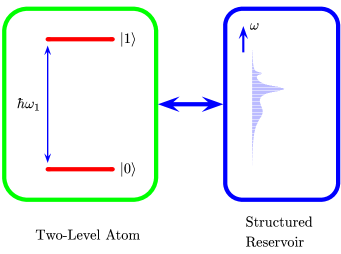
FIG. 1.: Illustration of a two-level atom coupled to a structured reservoir.

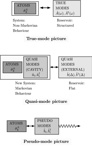
FIG. 2.: Three pictures of the coupled atomic system. In the true-mode picture the atom is coupled directly to true modes which have structure. In the quasi-mode picture the atoms are coupled to quasi-modes which are in turn coupled to external quasi-modes. In the pseudo-mode picture the atoms are coupled to dissipative pseudomodes.

REFERENCES

- [1] M. A. Nielsen and I. L. Chuang, Quantum Computation and Quantum Information (Cambridge University Press, Cambridge, 2000).
- [2] V. Vedral and M. B. Plenio, Prog. Quant. Electronics 22, 1 (1998).
- [3] A. M. Steane, Rep. Prog. Phys. 61, 117 (1997).
- [4] W. Zurek, Physics Today, October 1991, p36.
- [5] W. Zurek, Phys. Scripta, T76, 186 (1998).
- [6] A. Peres, Quantum Theory: Concepts and Methods, (Kluwer, Dortrecht, 1993).
- [7] C. J. Isham, Quantum Theory, (Imperial College Press, London, 1995).
- [8] D. P. DiVincenzo, Fortschr. Phys. 48, 771 (2000).
- [9] S. Haroche, Physics Today, July 1998, p36.
- [10] D. F. Walls and G. J. Milburn, Quantum Optics (Springer, Berlin, 1994).
- [11] M. O. Scully and M. S. Zubairy, Quantum Optics (Cambridge University Press, Cambridge, 1997).
- [12] S. M. Barnett and P. M. Radmore, Methods in Theoretical Quantum Optics (Oxford University Press, Oxford, 1997).
- [13] C. W. Gardiner, Quantum Noise (Springer, Berlin, 1991).
- [14] H. J. Carmichael, An Open Systems Approach to Quantum Optics (Springer-Verlag, Berlin, 1992).
- [15] I. Percival, Quantum State Diffusion (Cambridge University Press, Cambridge, 1998).
- [16] H. Haken, Light, Vol. 2: Laser Light Dynamics (North Holland, Amsterdam, 1981).
- [17] C. Cohen-Tannoudji and S. Haroche, J. Physique. 30, 125 (1969), ibid. 30, 153 (1969).
- [18] C. Cohen-Tannoudji and S. Reynaud, J. Phys. B: Atom. Mol. 10, 345 (1977).
- [19] G. Yeoman and S. M. Barnett, J. Mod. Opt. 43, 2037 (1996).
- [20] B. J. Dalton, Z. Ficek and S. Swain, J. Mod. Opt. 46, 379 (1999).
- [21] P. Lambropoulos, G. M. Nikolopoulos, T. R. Nielsen, and S. Bay, Rep. Prog. Phys. 63, 455 (2000).
- [22] T. W. Mossberg and M. Lewenstein, in Cavity Quantum Electrodynamics, ed. P. R. Berman, Adv. Atom. Mol. and Opt. Phys. S2 (1994), p171.
- [23] H. J. Kimble, in Cavity Quantum Electrodynamics, ed. P. R. Berman, Adv. Atom. Mol. and Opt. Phys. S2 (1994), p203.
- [24] Y. Wu, Phys. Rev. A61, 033803 (2000).
- [25] H. T. Dung and K. Ujihara, Phys. Rev. A60, 4067 (1999).
- [26] K. An, J. C. Childs, R. R. Dasari and M. S. Feld, Phys. Rev. Lett. 73, 3375 (1994).
- [27] Y. Mu and C. M. Savage, Phys. Rev. A46, 5944 (1992).
- [28] Y. Yamamoto and R. E. Slusher, Physics Today, June 1993, p66.
- [29] V. V. Klimov, M. Ducloy and V. S. Letokhov, Phys. Rev. A59, 2996 (1999).
- [30] V. B. Braginski, M. L. Gorodetsky and V. S. Ilchenko, Phys. Lett. A137, 393 (1989).
- [31] M. Woldeyohannes and S. John, Phys. Rev. A60, 5046 (1999).
- [32] E. Paspalakis, D. G. Angelakis, and P. L. Knight, Opt. Comm. 172, 229 (1999).
- [33] N. Vats and S. John, Phys. Rev. A 58, 4168 (1998).
- [34] Y. Yablonovitch, Phys. Rev. Lett. 58, 2059 (1987).
- [35] S. John, Phys. Rev. Lett. 58, 2486 (1987).
- [36] H. M. Wiseman and G. J. Milburn, Phys. Rev. Lett. 70, 548 (1993).
- [37] H. M. Wiseman, Phys. Rev. A49, 2133 (1994).
- [38] G. M. Nikolopoulos, S. Bay, and P. Lambropoulos, Phys. Rev. A 60, 5079 (1999).
- [39] R. Zwanzig, Physics 30, 1109 (1964).
- [40] S. Nakajima, Prog. Theor. Phys. 20, 948 (1958).
- [41] B. J. Dalton, J. Phys. A: Math. Gen. 15, 2157 (1982).
- [42] F. Shibata, Y. Takahashi, and H. Hashitsuma, J. Stat. Phys. 17, 171 (1977).
- [43] J. D. Cresser, Laser Phys. 10, 1 (2000).
- [44] H-P. Breuer, B. Kappler, and F. Petruccione, Phys. Rev. A 59, 1633 (1999).
- [45] W. Strunz, L. Diosi, and N. Gisin, Phys. Rev. Lett. 82, 1801 (1999).
- [46] M. W. Jack, M. J. Collett, and D. F. Walls, Phys. Rev. A 59, 2306 (1999).
- [47] K. Mølmer and S. Bay, Phys. Rev. A 59, 904 (1999).
- [48] T. Quang and S. John, Phys. Rev. A 56, 4273 (1997).
- [49] P. Stenius and A. Imamoglu, Quant. Semiclass. Opt. 8, 283 (1996).
- [50] S. Bay, P. Lambropoulos, and K. Mølmer, Phys. Rev. Lett. 79, 2654 (1997).
- [51] B. M. Garraway, Phys. Rev. A 55, 2290 (1997), ibid. A 55, 4636 (1997).
- [52] A. Imamoglu, Phys. Rev. A 50, 3650 (1994).
- [53] J. Jeffers, P. Horak, S. M. Barnett, and P. M. Radmore, Phys. Rev. A 62, 043602 (2000).
- [54] U. Fano, Phys. Rev. 124, 1866 (1961).
- [55] D. Braun, F. Haake, and W. T. Strunz, quant-ph/0006117 (2000).
- [56] B. J. Dalton, S. M. Barnett, and P. L. Knight, J. Mod. Opt. 46, 1315 (1999), ibid 1495 (1999).
- [57] S. M. Barnett and P. M. Radmore, Opt. Comm. 68, 364 (1988).
- [58] B. J. Dalton, E. S. Guerra, and P. L. Knight, Phys. Rev. A 54, 2292 (1996).
- [59] R. Lang, M. O. Scully, and W. E. Lamb Jr., Phys. Rev. A 7, 1788 (1973).
- [60] B. J. Dalton and P. L. Knight, J. Mod. Opt. 46, 1817 (1999), ibid 1839 (1999).
- [61] C. W. Gardiner and M. J. Collett, Phys. Rev. A 31, 3761 (1985).
- [62] S. Brown and B. J. Dalton, J. Mod. Opt. 47, (accepted for publication) (2001).
- [63] B. Huttner and S. M. Barnett, Phys. Rev. A46, 4306 (1992).
- [64] M. Rosenau da Costa, A. O. Caldeira, S. M. Dutra and H. Westfahl Jr., Phys. Rev. A61, 022107 (2000).
- [65] S. Bay, P. Lambropoulos, and K. Mølmer, Phys. Rev. A 57, 3065 (1998).