Thermal concurrence mixing in a 1D Ising model

Abstract

We investigate the entanglement arising naturally in a 1D Ising chain in a magnetic field in an arbitrary direction. We find that for different temperatures, different orientations of the magnetic field give maximum entanglement. In the high temperature limit, this optimal orientation corresponds to the magnetic field being perpendicular to the Ising orientation ($z$ direction). In the low temperature limit, we find that varying the angle of the magnetic field very slightly from the $z$ direction leads to a rapid rise in entanglement. We also find that the orientation of the magnetic field for maximum entanglement varies with the field amplitude. Furthermore, we have derived a simple rule for the mixing of concurrences (a measure of entanglement) due to mixing of pure states satisfying certain conditions.

I Introduction

Entanglement, the rather counterintuitive non-local correlations exhibited by quantum systems, has recently become one of the most valuable resources in quantum information processing bennett00 . Over the past few years it has developed into a quantifiable physical resource vedral97 ; bennett96 ; wootters98 in an analogous manner to energy. Thus, the amount of entanglement present naturally in complex physical systems (systems with many interacting components) now becomes a relevant question to ask. Condensed matter physicists have long investigated correlations between parts of composite systems. Entanglement is the “quantum” or “nonlocal” part of these correlations. As such, it can behave very differently from the total correlations. For example, while correlations are averaged on mixing states, entanglement generally decreases. The topic of variation of entanglement in condensed matter systems with respect to the variation of external parameters such as temperature, field components etc., is a relatively unexplored and potentially rich area of study. In this context, as a simple initial model, Arnesen, Bose and Vedral have studied the variation of entanglement with temperature and magnetic field in a 1D isotropic finite Heisenberg chain arnesen00 . Prior to that, Nielsen had investigated the entanglement between two qubits interacting via the Heisenberg interaction at a nonzero temperature nielsen98 and O’Connor and Wootters have investigated the entanglement in the ground state of an antiferromagnetic isotropic Heisenberg ring wootters00 . In Ref. arnesen00 , the entanglement at a nonzero temperature, being that of a thermal state, was called thermal entanglement. Subsequently, Wang has studied the quantum Heisenberg XY-model wang01 and the two-qubit anisotropic XXZ-model wang01b in a similar context.

In this paper, we are going to study the thermal entanglement in the 1D Ising model in an external magnetic field sachdev . Ising-like interactions form the basic coupling in many proposals for experimental systems that can be used to perform quantum computation, see for example, cory96 ; kane98 ; mooij99 ; briegel00 . The 1D Ising model describes a set of linearly arranged spins (qubits), each interacting with its nearest neighbors by a coupling which is proportional to $\sigma_{z}\otimes\sigma_{z}$. This coupling can be diagonalized in a basis of disentangled states. Naïvely one might think that this implies a complete absence of entanglement in the Ising model. However, an external magnetic field with a component, however small, along a direction perpendicular to the $z$ axis is sufficient to make the eigenstates entangled.

We start in section II by considering analytically the case of two qubits interacting via the Ising interaction in a magnetic field orthogonal to the $z$ direction. In section III, we formulate a theorem for the concurrence mixing due to occupation of both the ground and the excited states. Next, in section IV, we consider numerically the variation of entanglement with the orientation of magnetic field. Before concluding, in section V we show that the kinds of behavior found for two qubits also hold for many qubits.

II Two qubits with Ising interaction

The Hamiltonian for an isotropic quantum Ising model with nearest neighbor couplings in an external magnetic field can in the most general form be expressed as

$$\hat{H}=J\sum_{<i,j>}\hat{\sigma}_{z}^{i}\hat{\sigma}_{z}^{j}+\vec{B}\cdot\sum_{k}\vec{\hat{\sigma}^{k}},$$ (1)

where the indices $i$, $j$ and $k$ label the $N$ spins. Here we will consider systems in one spatial dimension with periodic boundary conditions so the $N$th spin also couples to the first spin. Thus we have a qubit “ring”. First we will consider the case of $N=2$. Our Hamiltonian can then be written as

$$\hat{H}=2J\,\hat{\sigma}_{z}\otimes\hat{\sigma}_{z}+\vec{B}\cdot(\vec{\hat{\sigma}}\otimes\hat{I}+\hat{I}\otimes\vec{\hat{\sigma}}).$$ (2)

The usual form of the Ising model has a magnetic field only along the $z$ axis. This case has no entanglement at all, since the Hamiltonian is diagonal in the standard disentangled basis $\{|00\rangle,|01\rangle,|10\rangle,|11\rangle\}$, where $|0\rangle$ stands for spin up and $|1\rangle$ stands for spin down. However, in this paper we will consider the cases when the magnetic field is not parallel to the $z$ axis.

II.1 Orthogonal fields

Let us first study the special case when the magnetic field is perpendicular to the $z$ axis, say $\vec{B}=B\,\vec{x}$. Our system is now described by the following Hamiltonian:

$$\hat{H}=2J\,\hat{\sigma}_{z}\otimes\hat{\sigma}_{z}+B\,(\hat{\sigma}_{x}\otimes\hat{I}+\hat{I}\otimes\hat{\sigma}_{x}).$$ (3)

We are going to investigate the entanglement in this two-qubit Ising ring. In this paper, we will use the squared concurrence wootters98 ; wootters00a , called the tangle $\tau$, as a measure of entanglement. To calculate this, first we need to define the product matrix $R$ of the density matrix, $\rho$, and its spin-flipped matrix, $\tilde{\rho}=(\hat{\sigma}_{y}\otimes\hat{\sigma}_{y})\rho^{*}(\hat{\sigma}_{y}\otimes\hat{\sigma}_{y})$. Hence, we have

$$R\equiv\rho\tilde{\rho}=\rho(\hat{\sigma}_{y}\otimes\hat{\sigma}_{y})\rho^{*}(\hat{\sigma}_{y}\otimes\hat{\sigma}_{y}).$$ (4)

Now concurrence is defined by

$$C=max\{\lambda_{1}-\lambda_{2}-\lambda_{3}-\lambda_{4},0\},$$ (5)

where the $\lambda_{i}$ are the square roots of the eigenvalues of $R$, in decreasing order. In this method the standard basis, $\{|00\rangle,|01\rangle,|10\rangle,|11\rangle\}$, must be used. As usual for entanglement measures, the tangle ranges from $0$ (no entanglement) to $1$, when the two qubits are maximally entangled.

For finite temperatures we need the density matrix, $\rho$, for a system which is at thermal equilibrium. This is given by $\rho=e^{-\hat{H}/T}/Z$, where $Z=tr(e^{-\hat{H}/T})$ is the partition function (using units where the Boltzmann constant, $k_{B}=1$). We then solve the time independent Schrödinger equation for our qubits. The energy levels of our Hamiltonian (3) are, in rising order, $-2\sqrt{J^{2}+B^{2}},-2J,2J,2\sqrt{J^{2}+B^{2}}$, as in Fig. 1.

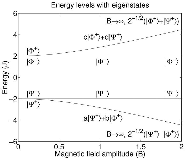
Figure 1: Energy levels with corresponding eigenstates, a,b,c and d are functions of B, and the states $|\Phi\pm\rangle=(|00\rangle\pm|11\rangle)/\sqrt{2}$ and $|\Psi\pm\rangle=(|01\rangle\pm|10\rangle)/\sqrt{2}$ are the four Bell states.

For zero temperature only the lowest energy level is populated. The tangle of this pure state can easily be calculated from the density matrix, for $B>0$,

$$\tau=\frac{J^{2}}{J^{2}+B^{2}}=\frac{1}{1+\left(\frac{B}{J}\right)^{2}}.$$ (6)

In Fig. 2, a contour plot of the tangle $\tau$, as a function of magnetic field amplitude, $B$, and the temperature, $T$ is shown.

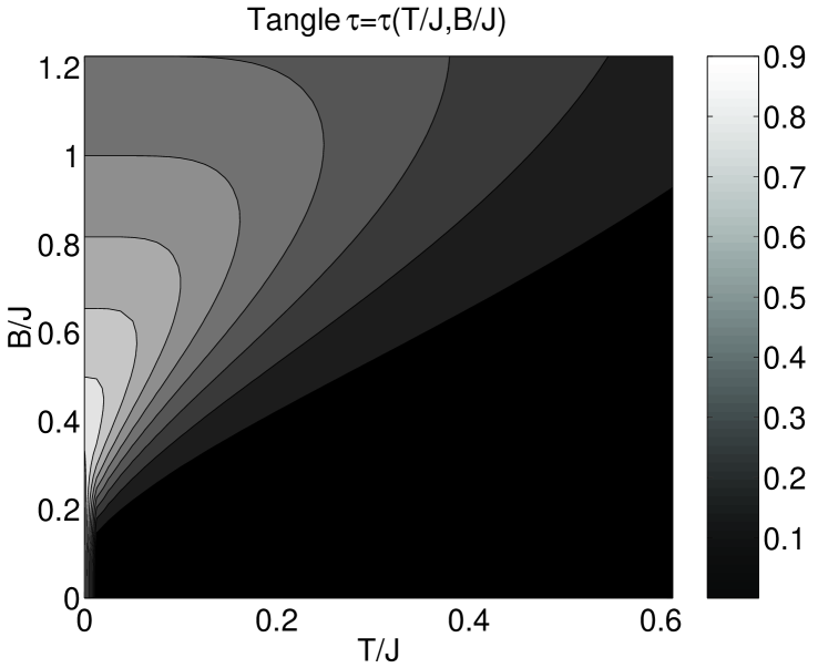
Figure 2: Contour plot of the tangle of two qubits obeying an Ising Hamiltonian with coupling $J$, in a perpendicular magnetic field $B$, for temperatures $T$.

From Eq. (6), it is clear that the entanglement is highest for nearly vanishing magnetic fields and decreases with increasing field amplitude. However, Eq. (6) is not valid for strictly $B=0$, in which limit it seems to predict maximal entanglement. At precisely $B=0$, in fact, no entanglement is present (the eigenstates are same as those of the usual Ising Hamiltonian without any magnetic field). Hence there is a quantum phase transition sachdev at the point B=0 when the entanglement jumps from zero to maximal even for an infinitesimal increase of $B$. As we will see later this point is only one point on a transition line for $B$-fields along the $z$ axis.

Let us now turn our attention to the more realistic case of non-zero temperatures. For a general pure state only one of the eigenvalues of Eq. (4) is non-zero and therefore equal to the tangle. This statement is proved in lemma 1 in the next section. For low temperature and magnetic field, i.e. $B,T\ll J$, it is a good approximation to assume that only the two lowest energy levels are populated. This becomes clear when we look at Fig. 1 in the regime $B\ll J$. The lowest two levels are much closer to each other compared with their separation from the third lowest energy level (i.e. the second excited state). Thus when the temperature is low, only the lowest two levels appear in the state of the system. We will find (theorem 1, next section) that, in our case, the combination of the two lowest states also combines their concurrences in the following weighted subtraction:

$$C=\max\{|w_{0}C_{0}-w_{1}C_{1}|,0\},$$ (7)

where the index $0$ refers to the ground state, while $1$ refers to the excited state and $w_{0}$ and $w_{1}$ are the weights of the ground and excited states respectively. The weights can be any weights from the statistics, for example Maxwell-Boltzmann statistics or Fermi-Dirac statistics. We call this concurrence mixing. In our case, the first excited state is the Bell state, $|\Psi^{-}\rangle=(|01\rangle-|10\rangle)/\sqrt{2}$, which has $\tau=1$, and Eq. (7) reduces to

$$C=|w_{0}\frac{J}{\sqrt{J^{2}+B^{2}}}-w_{1}|.$$ (8)

In general, the first term in the above equation is larger than the second, and in this case the concurrence decreases with temperature as $w_{0}$ decreases and $w_{1}$ increases (cf Fig. 2). In Fig. 2 we also see that, for a given temperature, the entanglement can be increased by adjusting the magnetic field and is generally largest for some intermediate value of the magnetic field. This effect can be understood by noting that $w_{0}$ increases with increasing $B$ as the energy separation between the levels increase, but $J/\sqrt{J^{2}+B^{2}}$ decreases. As a result the combined function reaches a peak as we vary $B$ and decreases subsequently, inducing analogous behavior for the concurrence.

III Concurrence mixing

In this section, we are going to formulate and prove a useful concurrence mixing theorem. We begin with a lemma which illustrates the method used in the theorem. The results of lemma 1 appear in Ref. wootters98 .

Lemma 1: Let $\rho$ be a pure density matrix. Then the product matrix $R=\rho\tilde{\rho}$, where $\tilde{\rho}=(\hat{\sigma}_{y}\otimes\hat{\sigma}_{y})\rho^{*}(\hat{\sigma}_{y}\otimes\hat{\sigma}_{y})$, has only one non-zero eigenvalue, and its value is the concurrence squared, i.e. the tangle. For a general pure state, $|\alpha\rangle=a|00\rangle+b|01\rangle+c|10\rangle+d|11\rangle$ the concurrence is $C=2|ad-bc|$ or, written as a Schmidt decomposition, $C=2|c_{0}c_{1}|$, where $c_{i}$ are the two Schmidt coefficients.

Proof: Consider a general pure density matrix $\rho=|\alpha\rangle\langle\alpha|$. By writing out the product matrix

$$\rho\tilde{\rho}=|\alpha\rangle\langle\alpha|\hat{\sigma}_{y}\otimes\hat{\sigma}_{y}|\alpha\rangle\langle\alpha|\hat{\sigma}_{y}\otimes\hat{\sigma}_{y},$$ (9)

we see directly that $|u_{0}\rangle=|\alpha\rangle$ is an eigenstate with eigenvalue $|\langle\alpha|\hat{\sigma}_{y}\otimes\hat{\sigma}_{y}|\alpha\rangle|^{2}$. It is always possible to find three more vectors $|\alpha_{k}^{\perp}\rangle,k=1,2,3$ all of them linearly independent of each other and orthogonal to $|\alpha\rangle$. Thus the remaining three eigenvectors can be written as $|u_{k}\rangle=\hat{\sigma}_{y}\otimes\hat{\sigma}_{y}|\alpha_{k}^{\perp}\rangle,k=1,2,3$, all with eigenvalue zero. From Eq. (5) we now get the concurrence to be $C=|\langle\alpha|\hat{\sigma}_{y}\otimes\hat{\sigma}_{y}|\alpha\rangle|=2|ad-bc|$. Thus, for a pure state, concurrence can be defined as the absolute expectation value of the operator $\hat{\sigma}_{y}\otimes\hat{\sigma}_{y}$. By tracing out one qubit and solving for the eigenvalues, which are equal to the square of the Schmidt coefficients, $c_{i}$, of the remaining density matrix, we find that the concurrence also can be written as $C=2|c_{0}c_{1}|$.

Theorem 1: Consider two pure states of the same system $|\alpha_{m}\rangle$ and $|\alpha_{n}\rangle$. If the spin-flip overlap is zero, i.e.

$$\langle\alpha_{m}|\hat{\sigma}_{y}\otimes\hat{\sigma}_{y}|\alpha_{n}\rangle=0,$$ (10)

then the concurrence of the mixture of the two pure states, with weights $w_{i}$, can be expressed as

$$C_{mixed}=|w_{m}C_{m}-w_{n}C_{n}|.$$ (11)

Proof: Let $\rho_{i}=|\alpha_{i}\rangle\langle\alpha_{i}|$, $i=m,n$, be our two pure states. From our lemma, we have

$$\rho_{i}\tilde{\rho_{i}}|u_{i0}\rangle =C_{i}^{2}|u_{i0}\rangle$$ (12)

$$\rho_{i}\tilde{\rho_{i}}|u_{ik}\rangle =0,\hskip 42.67912ptk=1,2,3$$ (13)

where $|u_{i0}\rangle=|\alpha_{i}\rangle$ and $|u_{ik}\rangle=\hat{\sigma}_{y}\otimes\hat{\sigma}_{y}|\alpha_{ik}^{\perp}\rangle$. Let us write our mixed state, $\rho$, as a weighted average of the pure density matrices, $\rho=w_{m}\rho_{m}+w_{n}\rho_{n}$. Since $\tilde{\rho}$ is only a linear transformation of $\rho$, we also have $\tilde{\rho}=w_{m}\tilde{\rho_{m}}+w_{n}\tilde{\rho_{n}}$. Using these assumptions, we can write down the product matrix

$$\rho\tilde{\rho}=w_{m}^{2}\rho_{m}\tilde{\rho_{m}}+w_{m}w_{n}(\rho_{m}\tilde{\rho_{n}}+\rho_{n}\tilde{\rho_{m}})+w_{n}^{2}\rho_{n}\tilde{\rho_{n}}.$$ (14)

Our condition (10) makes the cross terms drop out, since

$$\rho_{i}\tilde{\rho_{j}}=|\alpha_{i}\rangle\langle\alpha_{i}|\hat{\sigma}_{y}\otimes\hat{\sigma}_{y}|\alpha_{j}\rangle\langle\alpha_{j}|\hat{\sigma}_{y}\otimes\hat{\sigma}_{y}=0.$$ (15)

Furthermore, condition (10) together with Eq. (12) gives the following relation

$$\rho_{i}\tilde{\rho_{i}}|u_{j0}\rangle =|\alpha_{i}\rangle\langle\alpha_{i}|\hat{\sigma}_{y}\otimes\hat{\sigma}_{y}|\alpha_{i}\rangle\langle\alpha_{i}|\hat{\sigma}_{y}\otimes\hat{\sigma}_{y}|\alpha_{j}\rangle$$ (16)

$$=\delta_{ij}C_{j}^{2}|u_{j0}\rangle.$$

The Eqs. (14)-(16) give two of the four eigenequations of the product matrix

$$\rho\tilde{\rho}|v_{i}\rangle=(\delta_{im}w_{m}^{2}C_{m}^{2}+\delta_{in}w_{n}^{2}C_{n}^{2})|v_{i}\rangle,$$ (17)

where $|v_{i}\rangle=|u_{i0}\rangle=|\alpha_{i}\rangle$. Since these two eigenvectors only span two dimensions in the four-dimensional space, we can always find another two vectors $|\alpha_{k}^{\perp}\rangle,k=2,3$ which are linear independent of each other and orthogonal to the two eigenstates. Thus the last two eigenvectors are $|v_{k}\rangle=\hat{\sigma}_{y}\otimes\hat{\sigma}_{y}|\alpha_{k}^{\perp}\rangle,k=2,3$, both with zero eigenvalue. Eq. (5) now gives our mixed concurrence formula.

Theorem 1 applies to any system with a mixture of two pure states satisfying condition (10). It can easily be extended to apply to the mixing of more pure states. The requirement is then that condition (10) must hold for all pairs of pure states.

In our case, it would have been interesting if, when including all four levels, the concurrence could be calculated as

$$C=\max_{k}\{2w_{k}C_{k}-\sum_{i}w_{i}C_{i},0\}.$$ (18)

In fact, for a three-level approximation (involving the first three levels), this formula is correct, however the exact four-level concurrence is not in agreement with Eq. (18), because condition (10) does not hold for mixing the ground state with the third excited state.

IV Arbitrary fields

In section II we treated a case of a magnetic field orthogonal to the Ising direction. We are now going to generalize this to arbitrary magnetic fields. The new Hamiltonian can be written

$$\hat{H}= 2J\,\hat{\sigma}_{z}\otimes\hat{\sigma}_{z}$$ (19)

$$+B\sin\theta\,(\hat{\sigma}_{x}\otimes\hat{I}+\hat{I}\otimes\hat{\sigma}_{x})$$

$$+B\cos\theta\,(\hat{\sigma}_{z}\otimes\hat{I}+\hat{I}\otimes\hat{\sigma}_{z}),$$

where $\theta$ is the angle between the magnetic field and the Ising direction. It is sufficient to consider variation of $B$ in a plane containing the Ising direction, because in 3 spatial dimensions the Hamiltonian possesses rotational symmetry about the $z$ axis.

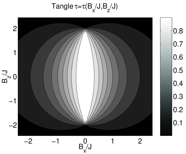
Figure 3: Contour plot of the tangle at zero temperature in a Cartesian coordinate system. Note that the line of non-entangled states at $B_{x}=0$ for $|B_{z}|<2J$ can not be seen.

The expression for the tangle is analytically solvable. However, because of a difficult cubic equation in the diagonalization, the expressions are complicated, so we present the results in graphical form. At zero temperature, Fig. 3 shows our solution when the tangle is plotted as a function of $B_{x}=B\sin{\theta}$ and $B_{z}=B\cos{\theta}$, and Fig. 4 shows the solution when the tangle is plotted as a function of the amplitude $B$ and angle $\theta$.

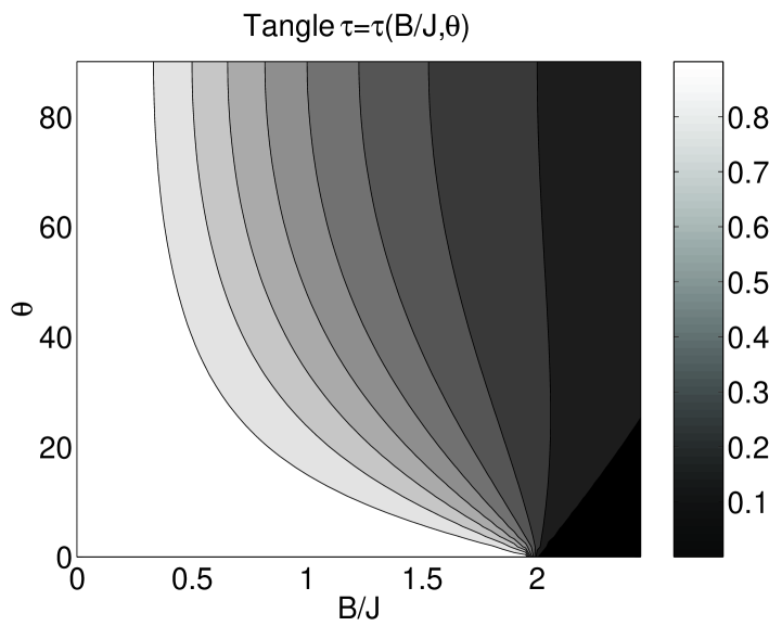
Figure 4: Contour plot of the tangle at zero temperature in a spherical coordinate system.

We notice that the region around $B_{x}=0$ for all $|B_{z}|<2J$ has the highest possible entanglement. At exactly at $B_{x}=0$ there should not be any entanglement, the white region of Fig. 3 indicates a quantum phase transition at $B_{x}=0$ (the sharpness of the transition being illustrated by the fact that the zero entanglement line at $B_{x}=0$ is so thin that it is invisible). For small angles, $\theta$, there are two energy levels close to the energy $-2J$ with corresponding states close to the Bell states $|\Psi^{\pm}\rangle=(|01\rangle\pm|10\rangle)/\sqrt{(}2)$. Thus we get a maximally entangled qubit pair in the limit. However, at $\vec{B}=B_{z}\vec{z}$, with $|B_{z}|<2J$, the states are degenerate with no entanglement as a result. In the case $B_{z}>2J$ ($B_{z}<-2J$) the ground state is always the non-entangled state $|11\rangle$ ($|00\rangle$). Also notice that $\theta=\pi/2$ corresponds to our earlier orthogonal case, thus the tangle follows Eq. (6). Even when $|B_{x}|$ is increased to the point where it starts to dominate, the spins will simply align along $B_{x}$ and give a disentangled state. Thus the entanglement falls off with increasing strength of the magnetic field in either direction.

Let us now look at the case of finite temperature (thermal entanglement). The first excited state is $|\Psi^{-}\rangle$ which lies at the energy $-2J$. This state is totally independent of magnetic field, thus the tangle corresponding to this state forms a constant plane at $1$. Fortunately, condition (10) in our theorem is also satisfied, which makes Eq. (7) valid. In Figs. 5 and 6 a numerical solution is shown at a low temperature. Note how fast the tangle drops to zero for a low $|B_{x}|$-component. This does not contradict the concurrence mixing formula, as the weights $w_{i}$ also depend on the magnetic field through the energy. The fast drop in the tangle is due to the degeneracy at $B_{x}=0$. The smallness of the energy difference at low values of $|B_{x}|$ makes the two levels almost equally populated even for small temperatures. The line of zero entanglement at $B_{x}=0$ for $T=0$ has broadened into a region of almost zero entanglement in the finite temperature case (compare Figs. 3, 5).

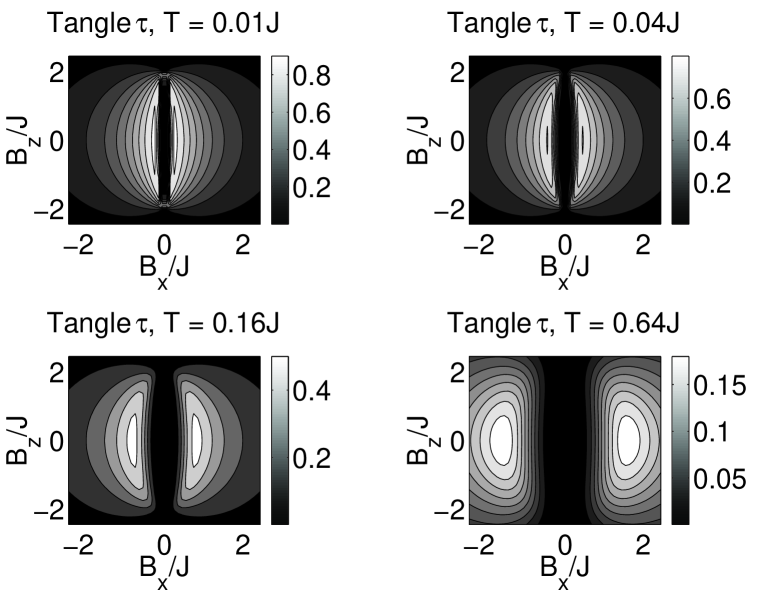
Figure 5: Contour plots of the tangle in Cartesian coordinates for various finite temperatures, $T$.

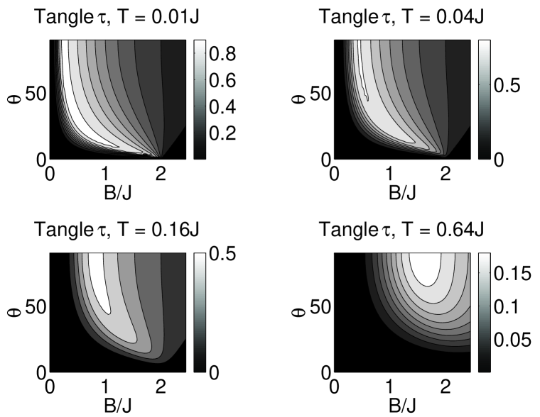
Figure 6: Contour plots of the tangle in spherical coordinates. The angle, resulting in the maximum entanglement for a given magnetic field amplitude, varies as a function of the amplitude and temperature.

It is also interesting to see that there exists an angle $\theta=\theta^{*}(B,T)$, where the entanglement is maximum for a given temperature and amplitude

$$\max\tau(\vec{B},T)=\tau(\theta^{*}(B,T)).$$ (20)

This feature can be explained heuristically if we assume that with $B_{x}$ and $B_{z}$ fixed, the entanglement should change continuously with temperature. We know that increasing the temperature widens the low entanglement zone around $B_{x}=0$ and the entanglement has to fall off for large $|B_{x}|$. So it is expected that at some intermediate value of $|B_{x}|$ (and hence $\theta$) the maximal entanglement will be reached. As we increase the temperature further, the near-zero entanglement zone centered around $B_{x}=0$ widens even more and pushes the entanglement maxima away to higher and higher values of $|B_{x}|$. The highest value of the tangle tends more and more towards orthogonal fields (c.f. Figs. 5, 6). The preferred angle traverses from $\theta=0$ at zero temperature (Fig. 4) to $\theta=\pi/2$ at $T\approx J$ (Fig. 6). In the classical limit, i.e. at very high temperatures all entanglement fades away as expected, because the state is completely mixed.

We can use the two-level approximation to get an estimate of the angle creating maximal entanglement. Let us first estimate the ground state energy, $\epsilon$. Since we know that the lowest two energy levels are very close and the first excited state is $-2J$, we can use the approximation $-2J+\epsilon\approx-4J$ while solving for eigenvalues of the Hamiltonian (19). The ground state energy is then

$$\epsilon=-2J-\frac{4B_{x}^{2}}{4J^{2}-B_{z}^{2}}J.$$ (21)

For the above approximation to hold, we must operate in a region not too close to the poles at $B_{z}=\pm 2J$. This gives the following energy difference between the two lowest levels

$$\Delta\epsilon=-2J-\epsilon\equiv\frac{4B_{x}^{2}}{4J^{2}-B_{z}^{2}}J.$$ (22)

The two terms of the ground state energy (21) can be considered as the first two terms in a Taylor expansion. This suggests that we instead write

$$\epsilon=-2J\sqrt{1+\frac{\Delta\epsilon}{J}}=-2J\sqrt{1+\frac{4B_{x}^{2}}{4J^{2}-B_{z}^{2}}}.$$ (23)

Let us, from here onwards, measure all energies in units of $J$, i.e. let $J=1$. For a magnetic field only in the $x$ direction, the concurrence of the ground state is $C_{0}=\tau^{1/2}=-2J/\epsilon$, where $\tau$ is given by Eq. (6). For non-zero $B_{z}$ this formula remains an excellent approximation (as we have verified numerically). Substituting Eq. (23) for $\epsilon$ gives

$$C_{0}=\frac{1}{\sqrt{1+\Delta\epsilon}}.$$ (24)

Recall that the first excited state is $|\Psi^{-}\rangle$ with concurrence $C_{1}=1$. From the concurrence mixing theorem (11) we get an approximation of the thermal concurrence. If $w_{i}$ are weights following Maxwell-Boltzmann statistics, then the maximum entanglement is reached when the following condition holds:

$$T(1+e^{\Delta\epsilon/T})=2(1+\Delta\epsilon+\sqrt{1+\Delta\epsilon}).$$ (25)

In the region we are interested in, where temperature is not bigger than $\sim 20\%$ of the coupling constant, $J$, the temperature is also much smaller than $\Delta\epsilon$, and Eq. (25) can be further simplified to

$$\Delta\epsilon=T\ln\frac{4}{T}.$$ (26)

Remember that the ground state energy is still a function of the magnetic field. In order to fix the temperature, $\Delta\epsilon$ has to be fixed, i.e. maximum entanglement is reached in the cross section between the energy surface and the constant energy plane that follows from Eq. (26). From Eq. (22) it is clear that this is described by an ellipse in a $B_{x}B_{z}$-plane. Using the field amplitude $B$ as a parameter, the angle we defined in Eq. (20) is given by

$$\sin\theta^{*}=\pm\sqrt{\frac{\Delta\epsilon}{4-\Delta\epsilon}\frac{4-B^{2}}{B^{2}}},$$ (27)

assuming that the parameter $|B|>\sqrt{\epsilon}$.

Another way to parameterize the optimum line is to let $B_{z}$ be the parameter and solve for $B_{x}$,

$$B_{x}=\pm\sqrt{\Delta\epsilon\left(1-\frac{B_{z}^{2}}{4}\right)},$$ (28)

with $|B_{z}|<2$. Again keep in mind that Eqs. (27) and (28) follow from the assumption that $\Delta\epsilon\approx 0$, and therefore the ellipse is not closed around the poles at $B_{z}=\pm 2$ (cf Figs. 5, 7).

V Qubit rings

As the expressions for the thermal tangle of the general two-qubit case are already quite complicated, we can not expect to find any easily manageable analytic expressions in the many-qubit case. Instead, we have performed numerical simulations, which gives the entanglement between neighboring qubits as shown in Fig. 7.

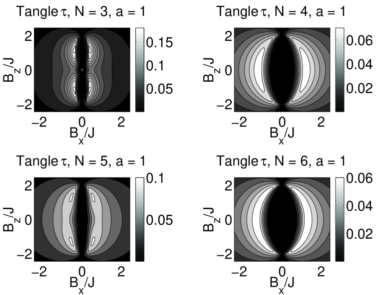
Figure 7: Contour plots of the tangle at temperature $T=0.10J$. N is the number of qubits in the chain and a=1 means that entanglement is measured between two neighboring qubits.

The behavior for even $N$ rings is quite similar to that of the two qubit case. To understand why there is an extra low entanglement zone around $B_{z}=0$ in the case of odd $N$ rings, one has to go back the basic cause for entanglement arising in the Ising chain. It results from the competition between the term $\hat{\sigma}_{z}\otimes\hat{\sigma}_{z}+B_{z}\hat{\sigma}_{z}$ trying to impose spin order in the $z$ direction and $B_{x}\hat{\sigma}_{x}$ trying to impose spin order in the $x$ direction. In the odd qubit case, it is impossible for all neighboring spins to be oriented oppositely, so the ordering power of $\hat{\sigma}_{z}\otimes\hat{\sigma}_{z}$ is significantly reduced. In such circumstances, it is mainly the competition between $B_{z}\hat{\sigma}_{z}$ and $B_{x}\hat{\sigma}_{x}$ (albeit aided by the small $\hat{\sigma}_{z}\otimes\hat{\sigma}_{z}$ interaction) which determines the entanglement. Thus the high entanglement values near $B_{z}=0$ present for the two qubit (and all other even $N$) cases disappear for odd $N$. Note also that the entanglement in the odd $N$ case is somewhat larger in magnitude compared with the even $N$ case. This is a result of the fact that the two terms $\hat{\sigma}_{z}\otimes\hat{\sigma}_{z}$ and $B_{z}\hat{\sigma}_{z}$ compete for the type of $z$ ordering (parallel or anti-parallel neighboring spins). In even $N$ case, this competition is much stronger and this tends to lower the entanglement by reducing the net effect of $z$ ordering terms with respect to $x$ ordering terms. As the number $N$ of qubits in the chain is increased, the difference between even and odd $N$ chains should disappear (because for large $N$, adding or removing an extra qubit from the chain should not make a significant difference). This effect is clearly seen in Fig. 7 where the difference in appearance between the plots for $N=3$ and $N=4$ is much greater than that between $N=5$ and $N=6$.

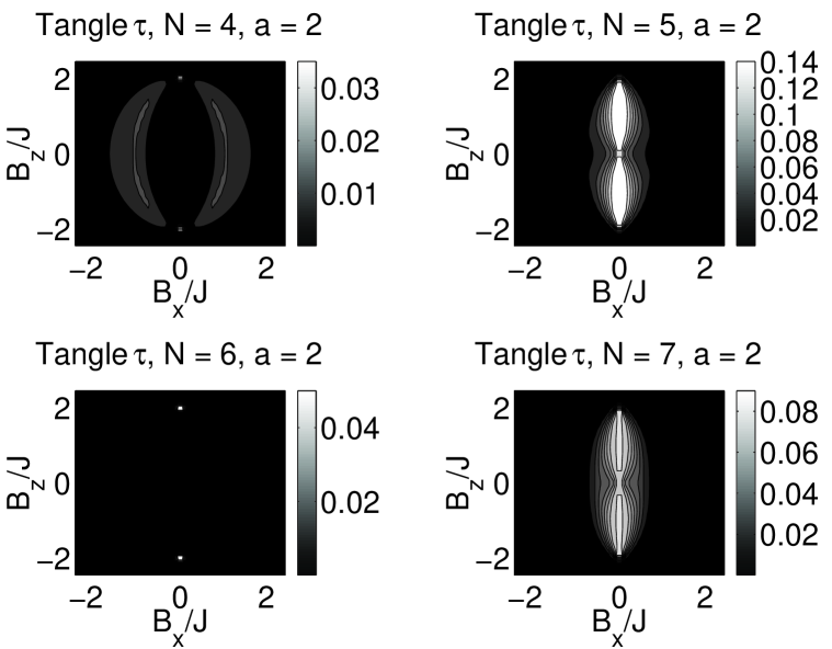
Figure 8: Contour plots of the tangle at temperature $T=0.10J$. N is the number of qubits in the chain and a=2 means that entanglement is measured in pairs with one qubit in-between.

Entanglement can also be calculated between non-neighboring qubits with the results shown in Fig. 8 for next-nearest neighbors. Again we observe that the even $N$ case has lower entanglement on average than the odd $N$ case. Also in the odd qubit case, the entanglement between next-nearest neighbors is somewhat complementary to that between nearest neighbors (this can be seen for example by placing the plots for $N=5$ in the two cases on top of each other). Thus the amount of entanglement between pairs of nearest neighbors and pairs of next-nearest neighbors can be controlled by varying the field direction.

VI Conclusions

In this paper we have investigated the natural thermal entanglement arising in an Ising ring with a magnetic field in an arbitrary direction. We have investigated two qubit analytically and three through seven qubits numerically. One of the most interesting results is the fact that for a given temperature, the (nearest neighbor, pairwise) entanglement in the ring can be maximized by rotating the magnetic field (at fixed magnitude) to an optimal direction. This can be regarded as magnetically induced entanglement. The pairwise entanglement between next-nearest neighbors can be maximized by rotating the field to a different direction. We have also proved a theorem of mixing of concurrences which is applicable to any system in which the pure states in the mixture have no spin-flip overlap.

So far we have have only considered pairwise entanglement. In future work we will estimate the entanglement between three or more qubits in the ring and also focus on investigating ways to detect the natural entanglement in Ising models, and on investigation of the entanglement in the large variety of available condensed matter models of interacting systems.

- (1) C. H. Bennett and D. P. DiVincenzo, Nature 404, 247 (2000).
- (2) V. Vedral, M. B. Plenio, M. A. Rippin and P. L. Knight, Phys. Rev. Lett. 78, 2275 (1997); V. Vedral and M. B. Plenio, Phys. Rev. A 57, 1619 (1998).
- (3) C. H. Bennett, H. J. Bernstein, S. Popescu and B. Schumacher, Phys. Rev. A 53, 2046 (1996); S. Popescu and D. Rohrlich, On the measure of entanglement for pure states, quant-ph/9610044.
- (4) W. K. Wootters, Phys. Rev. Lett 80, 2245 (1998).
- (5) M. C. Arnesen, S. Bose, V. Vedral, Natural thermal and magnetic entanglement in 1D Heisenberg model, quant-ph/0009060.
- (6) M. A. Nielsen, PhD Thesis, University of New Mexico (1998), quant-ph/0011036.
- (7) K. M. O’Connor and W. K. Wootters, Entangled rings, quant-ph/0009041; W. K. Wootters, Entangled chains, quant-ph/0001114.
- (8) X. Wang, Entanglement in the Quantum Heisenberg XY model, quant-ph/0101013.
- (9) X. Wang, Effects of anisotropy on thermal entanglement, quant-ph/0102072.
- (10) S. Sachdev, Quantum phase transitions (Cambridge University Press, Cambridge, 1999).
- (11) D. G. Cory, A. F. Fahmy, T. F. Havel, Nuclear magnetic resonance spectroscopy; an experimental accessible paradigm for quantum computing, Proceedings of the fourth Workshop on Physics and Computation (Complex Systems Institute, Boston, New England, 1996).
- (12) B. E. Kane, Nature 393, 133 (1998).
- (13) J. E. Mooij, T. P. Orlando, L. Levitov, L. Tian, C. H. van der Wal, S. Lloyd, Science 285, 1036 (1999).
- (14) H. J. Briegel, R. Raussendorf, Persistent entanglement in arrays of interacting particles, quant-ph/0004051; R. Raussendorf, H. J. Briegel, Quantum computing via measurements only, quant-ph/0010033.
- (15) In this paper we only consider entanglement between pairs of qubits, tangle thus refers to the 2-tangle throughout, V. Coffman, J. Kundu and W. K. Wootters, Phys. Rev. A 61, 052306 (2000).