ON FIRST-ORDER SCALING INTERTWINING IN QUANTUM MECHANICS

[Rev. Mex. Fís. 46 S2, (Nov. 2000) 153-156]

DAVID J. FERNÁNDEZ C.

Departamento de Física, CINVESTAV-IPN, Apdo Postal 14-740, 07000 México D.F., Mexico

HARET C. ROSU

Instituto de Física, Universidad de Guanajuato, Apdo Postal E-143, 37150 León, Gto, Mexico

Abstract. We generalize the standard first-order intertwining relationship of supersymmetric quantum mechanics in order to include simultaneous scaling transformations in both the original Hamiltonian and the intertwining operator. It is argued that in this way one can generate potentials with more interesting spectra than those obtained by means of the standard first-order intertwining technique and, as an outcome, a simple engineering procedure is presented. The harmonic oscillator potential is used in order to illustrate the previous statements. Moreover, a matrix representation of the scaled intertwining relationship is sketched up allowing for higher-dimensional generalizations in the case of separable potentials.

Resumen. Generalizamos la relación de entrelazamiento estandar de primer orden de la mecánica cuántica supersimétrica para incluir de manera simultánea transformaciones de escalamiento tanto en el Hamiltoniano original como en el operador de entrelazamiento. Se argumenta que en esta forma uno puede generar potenciales con espectros más interesantes que aquellos obtenidos por medio de la técnica de entrelazamiento estandar de primer orden y, como un resultado, un procedimiento sencillo de ingenieria cuántica es presentado. El potencial de oscilador armónico es usado para ilustrar las afirmaciones anteriores. Mas aún, una representación matricial de la relación de entrelazamiento escalado es bosquejado que permite la generalización a más de una dimensión en el caso de los potenciales separables.

Factorizations of second order linear one-dimensional (1D) differential operators are common tools in Witten’s supersymmetric quantum mechanics (SUSYQM) [?], which may be considered as a form of Darboux transformations [?]. They imply either particular solutions of Riccati equations known as superpotentials or the general Riccati solution (RS), the latter case being first used in physics by Mielnik for the quantum harmonic oscillator [?]. In recent years, it became clear that SUSYQM is not only a form of Darboux transformations but also a particular case in the more general framework provided by the technique of intertwining operators [?], of extensive use in the mathematical literature. Two (Hamiltonian) operators are said to be intertwined by an operator $A^{+}$ if the following relationship is fulfilled

$$H_{1}A^{+}=A^{+}H.$$ (1)

In SUSYQM $A^{+}$ is a first order differential (factorization) operator of the form

$$A^{+}=\frac{1}{\sqrt{2}}\left(-\frac{d}{dx}+\alpha(x)\right),$$ (2)

leading to the standard Riccati equation for $\alpha(x)$ associated to the given initial potential

$$\alpha^{\prime}(x)+\alpha^{2}(x)=2(V(x)-{\cal E}),$$ (3)

where the prime denotes derivative with respect to $x$. The potential $V_{1}(x)$ corresponding to $H_{1}$ is determined according to:

$$V_{1}(x)=V(x)-\alpha^{\prime}(x),$$ (4)

whenever one is able to find a solution of (3) for given $V(x)$ and ${\cal E}$. The so-called factorization energy ${\cal E}\in{\bf R}$ plays a crucial role in generating new solvable potentials from a given one. This becomes clear when substituting $\alpha(x)=[\ln\psi(x)]^{\prime}$ in (3), which leads to

$$H\psi(x)=-\frac{1}{2}\psi^{\prime\prime}(x)+V(x)\psi(x)={\cal E}\psi(x).$$ (5)

Although similar to the standard eigenvalue equation for $H$, notice that $\psi(x)$ in (5) is not necessarily normalizable, but it should not have zeros in order to avoid supplementary singularities of $V_{1}(x)$ with respect to those of $V(x)$. It is well known that for ${\cal E}>E_{0}$, where $E_{0}$ is the ground state energy of $H$, $\psi(x)$ will always have zeros. However, if ${\cal E}\leq E_{0}$ it is possible to make $\psi(x)$ to have no zeros by adjusting the ratio of the two constants in the general solution of (5), resulting in a physically meaningful $V_{1}(x)$ as explained for example by Sukumar [?]. The spectrum of $V_{1}(x)$ consists of the sequence of levels $E_{n}$ of the initial Hamiltonian plus a new ‘ground state’ energy level at ${\cal E}$. The scheme becomes complete after realizing that $H$ and $H_{1}$ are factorized in terms of $A$ and $A^{+}$ as follows:

$$H=AA^{+}+{\cal E},\qquad H_{1}=A^{+}A+{\cal E}.$$ (6)

If now one writes $H_{1}=H-f(x)$, the intertwining relationship (1) can be put in the commutator form as follows

$$[H,A^{+}]=f(x)A^{+},$$ (7)

and moreover, it is easy to see that Eq. (4) requires

$$f(x)=\alpha^{\prime}(x)~{},$$ (8)

that is, in the standard SUSYQM the function $f(x)$ is always the derivative of the RS $\alpha(x)$, and it will be called the Darboux potential difference (DPD) between the Darboux pair of almost isospectral potentials $V(x)$ and $V_{1}(x)$, respectively.

We now look for a more general first-order intertwining relationship and perform two simultaneous modifications: one related to the Hamiltonian in which we introduce a “perturbative” parameter $\epsilon$, $H_{1}=(1+\epsilon)H-f(x)$, and the other related to the intertwining operator (2) which is multiplied (say, to the right) by a unitary operator $U\equiv e^{i\frac{\lambda}{2}(xp+px)}$ ($U^{+}=U^{-1}$) depending on a ‘scaling’ real parameter $\lambda$:

$$A_{\lambda}^{+}=\frac{1}{\sqrt{2}}\left(-D+\alpha(x)\right)U,$$ (9)

where $D\equiv\frac{d}{dx}$. Multiplying Eq. (1) by $U^{+}$ to the right one gets

$$[(1+\epsilon)H-f(x)](-D+\alpha(x))=(-D+\alpha(x))UHU^{+},$$ (10)

and making equal on both sides of (10) the coefficients of the various corresponding powers of the derivative operator $D$ leads to

$$D^{3}: e^{-2\lambda}=1+\epsilon,$$ (11)

$$D^{2}: e^{-2\lambda}\alpha(x)=(1+\epsilon)\alpha(x),$$ (12)

$$D^{1}: (1+\epsilon)\alpha^{\prime}(x)+(1+\epsilon)V(x)-f(x)=V(e^{\lambda}x),$$ (13)

$$D^{0}: -\frac{(1+\epsilon)}{2}\alpha^{\prime\prime}(x)+[(1+\epsilon)V(x)-f(x)]\alpha(x)=\alpha(x)V(e^{\lambda}x)-V^{\prime}(e^{\lambda}x).$$ (14)

One can see that Eqs. (11) and (12) are the same, giving the relationship between the parameters $\epsilon$ and $\lambda$. After substituting $e^{-2\lambda}=1+\epsilon$, Eq. (13) reads

$$f(x)=e^{-2\lambda}\alpha^{\prime}(x)+e^{-2\lambda}V(x)-V(e^{\lambda}x)~{},$$ (15)

which is a more general form of Eq. (8). We can see that the original potential at two different points interfere in the connection between the DPD $f(x)$ and the RS $\alpha(x)$. This makes a key difference between the ‘scaling’ intertwining and the standard SUSYQM one, even for the cases when the potentials are homogeneous functions of degree $d$ for which (15) simplifies further to the more local form $f(x)=s^{-2}\alpha^{\prime}(x)+(s^{-2}-s^{d})V(x)$, where $s=e^{\lambda}$. When $d=-2$ one gets $f(x)=e^{-2\lambda}\alpha^{\prime}(x)$ which is the closest one can reach to the standard SUSYQM. Substituting Eqs. (11) and (15) in Eq. (14) and integrating it we get the Riccati equation

$$e^{-2\lambda}\alpha^{\prime}(x)+e^{-2\lambda}\alpha^{2}(x)=2(V(e^{\lambda}x)-\rm{\cal E})~{},$$ (16)

where, as it will be clear below, it is convenient to choose the integration constant equal to the factorization energy ${\cal E}$ of (3). Now, if one makes the change of variable $y=e^{\lambda}x$ and denotes $\tilde{\alpha}(y)=e^{-\lambda}\alpha(e^{-\lambda}y)$ one easily gets

$$\frac{d\tilde{\alpha}(y)}{dy}+\tilde{\alpha}^{2}(y)=2(V(y)-{\cal E}).$$ (17)

One can see that, up to a rescaling of the coordinate, this is the Riccati equation (3) with a factorization energy ${\cal E}$. Therefore, the same RS used in the standard intertwining technique (Eqs. (1) to (8)) can be used as well in the generalized scaling intertwining technique of Eqs.(1,9-17) in order to generate new solvable potentials with known spectra. The eigenfunctions of $H_{2}\equiv e^{2\lambda}H_{1}=H-e^{2\lambda}f(x)$ are proportional to the action of $A_{\lambda}^{+}$ on the eigenfunctions of $H$ due to the fact that the two Schrödinger Hamiltonians $H$ and $H_{2}$ are also intertwined, although now in a slightly generalized way:

$$H_{2}A_{\lambda}^{+}=e^{2\lambda}A_{\lambda}^{+}H.$$ (18)

The potential of the scaled intertwined Hamiltonian $H_{2}$ takes the form:

$$V_{2}(x)=V(x)-e^{2\lambda}f(x)=e^{2\lambda}V(e^{\lambda}x)-\alpha^{\prime}(x).$$ (19)

The corresponding eigenvalues are $\{e^{2\lambda}{\cal E},e^{2\lambda}E_{n}\}$, where $e^{2\lambda}{\cal E}$ is the ground state energy level of $H_{2}$ associated to the eigenfunction $\psi_{\cal E}(x)\propto\exp(-\int_{0}^{x}\alpha(z)dz)$. The factorizations of $H$ and $H_{2}$ in terms of $A_{\lambda}$ and $A_{\lambda}^{+}$ become:

$$H=e^{-2\lambda}A_{\lambda}A_{\lambda}^{+}+{\cal E},\qquad H_{2}=A_{\lambda}^{+}A_{\lambda}+e^{2\lambda}{\cal E}.$$ (20)

The generation of new exactly solvable potentials $V_{2}(x)$ by means of the scaling intertwining technique depends on the expertness to solve the Riccati equation (17). In particular, if either we find the general solution for just an isolated value of the factorization energy ${\cal E}$ or fixing it if we have the solution for ${\cal E}$ in a real interval, the family of potentials $V_{2}(x)$ derived by means of this technique would have the spectrum $\{e^{2\lambda}{\cal E},e^{2\lambda}E_{n}\}$, and by varying $\lambda$ we would be scaling the basic spectrum $\{{\cal E},E_{n}\}$ at $\lambda=0$ generated by means of the standard intertwining technique when creating a new level at ${\cal E}$ starting from the initial potential $V(x)$. However, the really interesting procedure is as follows. Suppose we would solve (17) for ${\cal E}$ belonging to a real interval $I=[{\cal E}_{1},{\cal E}_{2}]$, where ${\cal E}_{1}$ and ${\cal E}_{2}$ have the same sign. By choosing now ${\cal E}=e^{-2\lambda}{\cal E}_{0}$ with ${\cal E}_{0}\in I$ fixed and varying $\lambda$ such that always ${\cal E}\in I$, we would obtain potentials $V_{2}(x)$ having spectra of the type $\{{\cal E}_{0},(\frac{{{\cal E}}_{0}}{{\cal E}})E_{n}\}$, i.e., changed so that the excited state levels would be scaled while the ground state energy level of $H_{2}$ would be unaffected. This interesting effect is different of the one achieved by using the standard intertwining technique, where after solving the Riccati equation (3) for ${\cal E}$ belonging to a real interval, when varying ${\cal E}$ in its corresponding domain we would change the ground state energy level but maintaining unaffected the excited state levels. Thus, these two kinds of intertwining effects, alone or combined, provide us with considerable freedom for designing solvable potentials with suitable spectra for modeling purposes.

As an example, let us consider the harmonic oscillator potential $V(x)=x^{2}/2$. The solution to the Riccati equation (17) for an arbitrary ${\cal E}<1/2$ is given by (see, e.g., Sukumar and Junker and Roy [3]):

$$\tilde{\alpha}(y)=y+\frac{d}{dy}\bigg{\{}\!\ln\bigg{[}{}_{1}F_{1}\bigg{(}\frac{1+2{\cal E}}{4},\frac{1}{2};-y^{2}\bigg{)}+2\nu\frac{\Gamma(\frac{3-2{\cal E}}{4})}{\Gamma(\frac{1-2{\cal E}}{4})}\,y\,{}_{1}F_{1}\bigg{(}\frac{3+2{\cal E}}{4},\frac{3}{2};-y^{2}\bigg{)}\bigg{]}\bigg{\}},$$ (21)

where, in order to avoid singularities we have that $|\nu|<1$. Thus, the 3-parametric family of potentials (the parameters are $\lambda,\ {\cal E},\ \nu$),

$$V_{2}(x)=e^{4\lambda}\frac{x^{2}}{2}-e^{\lambda}\tilde{\alpha}^{\prime}(e^{\lambda}x),$$ (22)

with $\tilde{\alpha}(y)$ given by (21), has spectrum $\{e^{2\lambda}{\cal E},e^{2\lambda}(n+1/2),n=0,1,\dots\}$. By varying $\lambda$ and maintaining ${\cal E}$ fixed, we will move into members of the family (22) attainable after applying the scale transformation onto the potentials generated by means of the standard intertwining technique, which have spectrum $\{{\cal E},E_{n}=n+1/2,n=0,1,\dots\}$. On the other hand, if we take ${\cal E}=e^{-2\lambda}{\cal E}_{0}\in I_{1}=(-\infty,0)$, where ${\cal E}_{0}\in I_{1}$ is fixed, when varying the scaling parameter $\lambda$ we would be changing ${\cal E}$ so that one will get a two-parameter family of potentials with spectrum $\{{\cal E}_{0},(\frac{{\cal E}_{0}}{{\cal E}})(n+1/2),n=0,1,\dots\}$, i.e., the excited state levels will be scaled by the factor ${\cal E}_{0}/{\cal E}$, but the ground state energy level will remain fixed. A similar treatment can be implemented for ${\cal E}\in I_{2}=(0,1/2)$. A plot of the potentials $V_{2}(x)$ as a function of $x$ and ${\cal E}\in I_{1}$, with ${\cal E}_{0}=-1/2$ and $\nu=0$, is shown in Figure 1. Notice that this selection of ${\cal E}_{0}$ and $\nu$ ensures that, up to a displacement of the energy origin, the oscillator potential is included in this family (for ${\cal E}=-1/2$, i.e., $\lambda=0$), and for other values of ${\cal E}$ $V_{2}(x)$ is symmetric with respect to $x=0$. For ${\cal E}\in(-1/2,0)$ the potentials $V_{2}(x)$ have a double well, and the corresponding spacing for the excited state levels is expanded by the factor $-1/(2{\cal E})$ ($1$ is the original spacing of the oscillator potential). The ground state energy level in this case is fixed at $-1/2$. On the other hand, for ${\cal E}\in(-\infty,-1/2)$, the potentials $V_{2}(x)$ present just a peaked single well centered at $x=0$, which can be seen as a deformation of the well of the oscillator potential $x^{2}/2-1$ needed to maintain fixed the ground state energy level at $-1/2$. The excited state levels are ‘squeezed’ by the factor $-1/(2{\cal E})$.

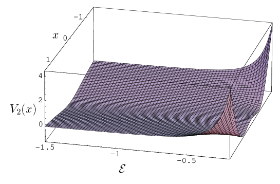
Figure 1: Plot of the potentials $V_{2}(x)$ of (22) as a function of $x$ and ${\cal E}$ when $e^{2\lambda}=-1/(2{\cal E})$ and $\nu=0$. The oscillator potential $x^{2}/2-1$ is a member of this family arising for ${\cal E}=-1/2$.

In interesting works, Spiridonov [?] has used a rather similar type of scaling intertwining in a different notation (the $q$ one) for emphasizing the connection between the $q$-deformed calculus [?] and Shabat’s infinite chain of reflectionless potentials [?]. In such a treatment the so-called self-similar potentials have been introduced and characterized, and at the same time the corresponding spectrum has been determined by means of the algebraic technique itself. On the other hand, in this paper the orientation has been different: to take initially a potential with known spectrum in order to generate a new potential with known and different (in general) spectrum. Since in the limit $\lambda\rightarrow 0$ we recover the results derived by means of the standard first order intertwining, we have at hand an appropriate and interesting generalization of such a technique. For any other $\lambda$ the new spectrum will not have common elements with the initial one, and moreover, the above mentioned non-local influence of the initial potential on the DPD (see Eq. (15)) will be at work. This is one of the interesting novelties put forth by means of scaling/deformation within the SUSYQM intertwining procedure.

The generalization of the scaled intertwining formalism to more dimensions can be easily performed for the cases when one deals with separable potentials by means of the matrix representation [?]. Thus, for separable 2D potentials one introduces ${\cal A}^{-}=\left(\begin{array}[]{cc}A&0\\ 0&B\end{array}\right)$ and ${\cal A}^{+}=\left(\begin{array}[]{cc}A^{+}&0\\ 0&B^{+}\end{array}\right)$. The symbols $A$ and $B$ denote the factorization operators for the first and second coordinate axis, respectively. The 2$\times$2 matrix intertwining relationship corresponding to (1) reads

$${\cal H}_{1}{\cal A}^{+}={\cal A}^{+}{\cal H},$$ (23)

where

$${\cal H}=\pmatrix{AA^{+}+{\cal E}_{1}&0\cr 0&BB^{+}+{\cal E}_{2}\cr}.$$ (24)

Corresponding to the function $f(x)$ and the unitary operator $U$ one introduces the following 2$\times$2 diagonal matrices

$${\cal F}=\pmatrix{f_{1}(x)&0\cr 0&f_{2}(y)\cr}=\pmatrix{\alpha^{\prime}_{1}(x)&0\cr 0&\alpha^{\prime}_{2}(y)\cr}$$ (25)

and

$${\cal U}=\pmatrix{e^{i\frac{\lambda_{1}}{2}(xp_{x}+p_{x}x)}&0\cr 0&e^{i\frac{\lambda_{2}}{2}(yp_{y}+p_{y}y)}\cr}~{},$$ (26)

respectively. In (26) the two scaling parameters may or may not be equal. By means of these matrices, all the 1D formulas of this paper have 2$\times$2 matrix counterparts, though one can immediately see that in order to maintain the diagonality of matrices one needs separable potentials. As an example, the matrix form of equation (7) reads $[{\cal H},{\cal A}^{+}]={\cal F}{\cal A}^{+}$. It is also quite easy to generalize this matrix representation to any number of even dimensions.

Finally, we draw attention to the fact that the scaling intertwining formalism could be applied to any type of Hamiltonians displaying scaling properties, not necessarily quantum ones. On the other hand, many interesting 2D cases are not separable. We recall as an example the diamagnetic Kepler problem, i.e., the Hamiltonian problem of the hydrogen atom in a magnetic field [?], that in atomic units ($\hbar=e=m_{e}=1$) and for zero angular momentum reads $H=\frac{1}{2}{\bf p}^{2}+\frac{1}{8}\gamma^{2}(x^{2}+y^{2})-\frac{1}{r}$, where $\gamma=B$/(2.35$\times$$10^{5}$T) gives the magnetic field strength. In scaled coordinates and momenta, $\tilde{{\bf r}}=\gamma^{2/3}{\bf r}$ and $\tilde{{\bf p}}=\gamma^{-1/3}{\bf p}$, respectively, this Hamiltonian can be written $\tilde{H}=\gamma^{-2/3}H$ and does not depend on the energy and field strength separately, but only on the scaled energy $\tilde{E}=\gamma^{-2/3}E$. This case, which is also of much laboratory and astrophysical interest, despite its scaling features, might be suitable for a more general scaling intertwining approach with coupled Riccati equations and non-diagonal matrices. Since here our purposes are merely illustrative we refer the reader to our recent preprint [?] for more complicated cases.

Acknowledgements

This work was supported in part by the CONACyT Projects 26329-E and 458100-5-25844E. HCR wishes to thank for the kind hospitality at the Departamento de Física, CINVESTAV.

References

References

- [1] Witten E 1981 Nucl. Phys. B 185 513. For a recent review, see Cooper F, Khare A and Sukhatme U 1995 Phys. Rep. 251 267
- [2] Darboux G 1882 C.R. Acad. Sci. 94 1456; For book, Matveev V B and Salle M A 1991 Darboux Transformations and Solitons (New York: Springer)
- [3] Mielnik B 1984 J. Math. Phys. 25 3387; Nieto M M 1984 Phys. Lett. B 145 208; Fernández D J 1984 Lett. Math. Phys. 8 337; Sukumar C V 1985 J. Phys. A 18 2917; for recent extensions and applications see Fernández D J, Glasser M L and Nieto L M 1998 Phys. Lett. A 240 15; Fernández D J, Hussin V and Mielnik B 1998 Phys. Lett. A 244 309; Rosu H C 1996 Phys. Rev. A 54 2571; 1997 Phys. Rev. E 56 2269; Rosu H C and Reyes M 1998 Phys. Rev. E 57 4850; Drigo-Filho E and Ruggiero J R 1997 Phys. Rev. E 56, 4486; Rosas-Ortiz O 1998 J. Phys. A 31 L507 and 10163; Márquez I F, Negro J and Nieto L M 1998 J. Phys. A 31 4115; Junker G and Roy P 1998 Ann. Phys. 270 155
- [4] See for example, Deift P A 1978 Duke Math. J. 45 267 and references therein; Anderson A 1991 Phys. Rev. A 43 4602
- [5] Spiridonov V 1992 Phys. Rev. Lett. 69 398; Mod. Phys. Lett. A7 1241; See also Section 5 in Andrianov A A, Ioffe M V, Cannata F and Dedonder J-P 1995 Int. J. Mod. Phys. A 10 2683
- [6] For books, Chaichian M and Demichev A 1996 Introduction to Quantum Groups (Singapore: World Scientific); Biedenharn L C and Lohe M A 1995 Quantum Group Symmetry and q-Tensor Algebras (Singapore: World Scientific)
- [7] Shabat A 1992 Inverse Problems 8 303
- [8] Rosu H C and Reyes M 1995 Phys. Rev. E 51 5112
- [9] Friedrich H and Wintgen D 1989 Phys. Rep. 183 37
- [10] Fernández D J and Rosu H C 1999, quant-ph/9910125 (submitted for publication)