A modified de Broglie-Bohm (dBB) approach to quantum mechanics is presented. In this new deterministic theory, the problem of zero velocity for bound states does not appear. Also this approach is equivalent to standard quantum mechanics when averages of dynamical variables are taken, in exactly the same way as in the original dBB theory.

PACS No(s): 03.65.Bz

In the de Broglie-Bohm quantum theory of motion (dBB) [1], which provides a deterministic theory of motion of quantum systems, the following assumptions are made [2]:

(A1) An individual physical system comprises a wave propagating in space and time, together with a point particle which moves continuously under the guidance of the wave.

(A2) The wave is mathematically described by $\Psi(x,t)$, a solution to the Schrodinger’s wave equation.

(A3) The particle motion is obtained as the solution $x(t)$ to the equation

$$\dot{x}=\frac{\hbar}{2im}\frac{\left(\Psi^{\star}\frac{\partial\Psi}{\partial x}-\frac{\partial\Psi^{\star}}{\partial x}\Psi\right)}{\Psi^{\star}\Psi},$$ (1)

with the initial condition $x=x(0)$. An ensemble of possible motions associated with the same wave is generated by varying $x(0)$.

(A4) The probability that a particle in the ensemble lies between the points $x$ and $x+dx$ at time $t$ is given by $\Psi^{\star}\Psi\;dx$.

In spite of its success as a deterministic theory, this scheme has the drawback that for many bound state problems of interest, in which the time-independent part $\psi$ of the wave function is real, the velocity of the particle turns out to be zero; i.e., the particle is at rest whereas classically one would expect it to move [2].

To have a better understanding of this problem, let us recall that in the the classical Hamilton-Jacobi theory, the trajectory for a particle is obtained from the equation

$$\frac{\partial S}{\partial t}+H\left(x,\frac{\partial S}{\partial x}\right)=0$$ (2)

by first attempting to solve for the Hamilton-Jacobi function $S=W-Et$ and then integrating the equation of motion

$$p=m\dot{x}=\frac{\partial S}{\partial x}$$ (3)

with respect to time. However, since the classical Hamilton-Jacobi equation is not adequate to describe the micro world, one resorts to the Schrodinger equation $i\hbar\partial\Psi/\partial t=-(\hbar^{2}/2m)\partial^{2}\Psi/\partial x^{2}+V\Psi$ and solves for the wave function $\Psi$. The basic idea of dBB is to put $\Psi$ in the form $Re^{iS/\hbar}$ and then to identify $S$ as the Hamilton-Jacobi function. The particle velocity is then given by Eq. (3) above, and this leads to Eq. (1). For wave functions whose space part is real, the Hamilton’s characteristic function $W=constant$ and hence the velocity field is zero everywhere, which is the problem mentioned above.

Another deterministic approach to quantum mechanics, which also claims the absence of this problem, is the trajectory representation developed by Floyd [3]. In one dimension, Floyd uses the generalized Hamilton-Jacobi equation

$$\frac{(W^{\prime})^{2}}{2m}+V-E=-\frac{\hbar^{2}}{4m}\left[\frac{W^{\prime\prime\prime}}{W^{\prime}}-\frac{3}{2}\left(\frac{W^{\prime\prime}}{W^{\prime}}\right)^{2}\right],$$ (4)

where $W^{\prime}$ (^′ denotes $\frac{\partial}{\partial x}$) is the momentum conjugate to $x$. Recently Faraggi and Matone [4] have independently generated the same equation (referred to as the quantum stationary Hamilton-Jacobi equation) from an equivalence principle free from any axioms. The general solution to this nonlinear equation is given by [3]

$$W^{\prime}=\pm(2m)^{1/2}(a\phi^{2}+b\theta^{2}+c\phi\theta)^{-1},$$ (5)

where ($\phi$, $\theta$) is a set of normalized independent solutions of the associated time-independent Schrodinger equation and ($a$, $b$, $c$) is a set of real coefficients such that $a,\;b>0$. Floyd argues that the conjugate momentum $W^{\prime}$ is not the mechanical momentum; instead, $m\dot{x}=m\partial E/\partial W^{\prime}$. The equation of motion in the domain [$x,t$] is rendered by the Jacobi’s theorem. For stationarity, the equation of motion for the trajectory time $t$, relative to its constant coordinate $\tau$, is given as a function of $x$ by [3, 4, 5]

$$t-\tau=\frac{\partial W}{\partial E},$$ (6)

where the trajectory is a function of ($a$, $b$, $c$) and $\tau$ specifies the epoch. Each of these non unique trajectories manifest a microstate of the Schrodinger wave function, even for bound states. Thus the Bohmian and trajectory representations differ significantly in the use of the equation of motion, though they are based on equivalent generalized Hamilton-Jacobi equations. The trajectory representation does not claim equivalence with standard quantum mechanics in the predictions of all observed phenomena nor does it explain the concept of probability density inherent in the Copenhagen interpretation.

In this Brief Report, we present a different and modified version of the dBB that surmounts the problem mentioned in the introduction. In addition, it is closer to the classical Hamilton-Jacobi theory than even the conventional dBB. We apply the scheme to a few simple problems and find that it is capable of providing a deeper insight into the quantum phenomena. Also it is shown that like dBB, the new scheme is equivalent to standard quantum mechanics when averages of dynamical variables are taken.

To this end, we first note that in the dBB, the substitution $\Psi=Re^{iS/\hbar}$ in the Schrodinger equation gives rise to two coupled partial differential equations, one of which contains an unknown quantum potential term, and this leads to a situation apparently different from the classical Hamilton-Jacobi theory for individual particles. On the other hand, we note that a change of variable $\Psi\equiv{\cal N}e^{iS/\hbar}$ in the Schrodinger equation (where ${\cal N}$ is a constant) gives a quantum-mechanical Hamilton-Jacobi equation [6]

$$\frac{\partial S}{\partial t}+\left[\frac{1}{2m}\left(\frac{\partial S}{\partial x}\right)^{2}+V\right]=\frac{i\hbar}{2m}\frac{\partial^{2}S}{\partial x^{2}},$$ (7)

which is closer to its classical counterpart and which also has the correct classical limit. This substitution brings the classical expression (3) for the conjugate momentum to the form

$$m\dot{x}=\frac{\hbar}{i}\frac{1}{\Psi}\frac{\partial\Psi}{\partial x}.$$ (8)

We therefore attempt to modify the dBB scheme in a manner similar to the latter approach; i.e., we retain assumptions A1, A2 and A4 whereas in A3, we identify $\Psi\equiv{\cal N}e^{iS/\hbar}$ and use the expression (8) as the equation of motion.

To see how the scheme works, let us consider the example of the ground state solution $\Psi_{0}$ of the Schrodinger equation for the harmonic oscillator in one dimension, the space part of which is real. We have

$$\Psi_{0}={\cal N}_{0}e^{-\alpha^{2}x^{2}/2}e^{-iE_{0}t/\hbar}.$$ (9)

The velocity field in the new scheme is given by Eq. (8) as

$$\dot{x}=-\frac{\hbar}{im}\alpha^{2}x,$$ (10)

whose solution is

$$x=Ae^{i\hbar\alpha^{2}t/m}.$$ (11)

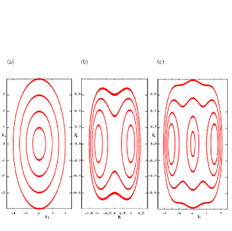
This is an equation for a circle of radius $|A|=|x(0)|$ in the complex plane [Fig. 1(a)]. As usual in such mechanical problems, we take the real part of this expression,

$$x_{r}=A\cos(\hbar\alpha^{2}t/m)$$ (12)

[where it is chosen that at $t=0$, $x(0)\equiv A$ is real], as the physical coordinate of the particle. It shall be noted that this is the same classical solution for a harmonic oscillator of frequency $\omega_{0}=\hbar\alpha^{2}/m$.

We can adopt this procedure to obtain the velocity field, also for higher values of the quantum number n. For $n=1$, we have

$$\Psi_{1}={\cal N}_{1}e^{-\alpha^{2}x^{2}/2}\;2\alpha x\;e^{-iE_{1}t/\hbar},$$ (13)

from which

$$\dot{x}=\frac{\hbar}{im}\left(-\alpha^{2}x+\frac{1}{x}\right).$$ (14)

The solution to this equation can be written as

$$(\alpha x-1)(\alpha x+1)=Ae^{2i\hbar\alpha^{2}t/m}$$ (15)

or

$$x=\frac{1}{\alpha}\sqrt{1+Ae^{2i\hbar\alpha^{2}t/m}}.$$ (16)

Here, the solution is a product of two circles centered about $\alpha x=\pm 1$, which is plotted in Fig. 1(b). The physical coordinate of the particle is again given by the real part of this expression. For $n=2$, the solution can similarly be constructed as

$$4\alpha x\left(\alpha x-\sqrt{5/2}\right)^{2}\left(\alpha x+\sqrt{5/2}\right)^{2}=Ae^{5i\hbar\alpha^{2}t/m}.$$ (17)

The trajectory in the complex plane is plotted in Fig. 1(c). Note that in all these cases, the velocity fields are not zero everywhere.

Now let us apply the procedure to some other stationary states which have complex wave functions. For a plane wave, we have

$$\Psi=Ae^{ikx}e^{-iEt/\hbar},$$ (18)

so that $\dot{x}=\hbar k/m$ and this gives

$$x=x(0)+\frac{\hbar k}{m}t,$$ (19)

the classical solution for a free particle.

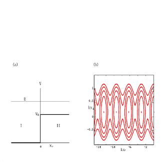
As another example, consider a particle with energy $E$ approaching a potential step with height $V_{0}$, shown in Fig. 2(a). In region I, we have

$$\psi_{I}=e^{ikx}+Re^{-ikx},\qquad k=\sqrt{2mE/\hbar^{2}}$$ (20)

and in region II,

$$\psi_{II}=Te^{iqx},\qquad q=\sqrt{2m(E-V_{0})/\hbar^{2}}.$$ (21)

The velocity fields in the two regions are given by

$$\dot{x}_{I}=\frac{\hbar k}{m}\left(\frac{e^{ikx}-Re^{-ikx}}{e^{ikx}+Re^{-ikx}}\right)$$ (22)

and

$$\dot{x}_{II}=\frac{\hbar q}{m},$$ (23)

respectively. The contours in the complex $x$-plane in region I, for a typical value of the reflection coefficient $r\equiv R^{2}=1/2$, are given by

$$\sqrt{2}\cos 2kx_{Ir}-e^{2kx_{Ii}}-\frac{1}{2}e^{2kx_{Ii}}=c$$ (24)

[where $x_{Ir}$ and $x_{Ii}$ are, respectively, the real and imaginary parts of $x_{I}$], and are plotted in Fig. 2(b). Note that also this case is significantly different from the corresponding dBB solution.

Lastly, we consider a nonstationary wave function, which is a spreading wave packet. Here, let the propagation constant $k$ has a Gaussian spectrum with a width $\Delta k\sim 1/\sigma$ about a mean value $\bar{k}$. The wave function is given by

$$\Psi(x,t)={\cal N}\left(\frac{2\pi\sigma}{\sigma^{2}+i\hbar t/m}\right)^{1/2}\exp\left[-\frac{(x-i\sigma^{2}\bar{k})^{2}}{2(\sigma^{2}+i\hbar t/m)}-\frac{\sigma^{2}+\bar{k}^{2}}{2}\right].$$ (25)

The velocity field is obtained from (8) as

$$\dot{x}=-\frac{\hbar}{im}\left(\frac{x-i\sigma^{2}\bar{k}}{\sigma^{2}+i\hbar t/m}\right)$$ (26)

Integrating this expression, we get

$$x(t)=x(0)+\frac{\hbar\bar{k}}{m}t+i\frac{\hbar}{m}\frac{x(0)}{\sigma^{2}}t.$$ (27)

Separating the real and imaginary parts of this equation (and assuming $\bar{k}$ is real), we get,

$$x_{r}(t)=x_{r}(0)+\frac{\hbar\bar{k}}{m}t+\frac{\hbar}{m}\frac{x_{i}(0)}{\sigma^{2}}t$$ (28)

and

$$x_{i}(t)=x_{i}(0)+\frac{\hbar}{m}\frac{x_{r}(0)}{\sigma^{2}}t.$$ (29)

For the particle with $x(0)=0$, we obtain $x_{r}(t)=(\hbar\bar{k}/m)t$ and $x_{i}(t)=0$; i.e., this particle remains at the center of the wave packet. Other particles assume different positions $x(t)$ at time $t$ as given by the above expression, which indicates the spread of the wave packet.

A new element in the present approach to quantum mechanics (though it is quite familiar in elementary mechanical problems) is that the particle coordinates are having real and imaginary parts. Similar is the case for the velocity, given by Eq. (8). If we are interested in the real part of this velocity, then one can write

$$\dot{x}_{r}=\frac{\hbar}{2im}\frac{\left[\Psi^{\star}\frac{\partial\Psi}{\partial x}-(\frac{\partial\Psi}{\partial x})^{\star}\Psi\right]}{\Psi^{\star}\Psi},$$ (30)

an expression quite analogous to the expression for velocity field in the dBB scheme (though not identical with it). One can also write $\dot{x}_{r}$ as

$$\dot{x}_{r}=\frac{\hbar}{2im}\frac{\left[\Psi^{\star}\frac{\partial\Psi}{\partial x_{r}}-(\frac{\partial\Psi}{\partial x_{r}})^{\star}\Psi\right]}{\Psi^{\star}\Psi},$$ (31)

where use is made of the fact that for complex derivatives, $\frac{\partial\Psi}{\partial x}=\frac{\partial\Psi}{\partial x_{r}}$. This equation is identical to the dBB velocity field at all points $x=x_{r}$.

Now consider an ensemble of particles, whose initial density function along $x=x_{r}$ is given by

$$P(x_{r},t=0)=\Psi^{\star}(x=x_{r},t=0)\Psi(x=x_{r},t=0).$$ (32)

Now let us ask whether $P(x_{r},t)=\Psi^{\star}(x=x_{r},t)\Psi(x=x_{r},t)$ be identified as the density function along $x=x_{r}$ at any time $t$, given the velocity field (8). For this to be in the affirmative, the conservation equation

$$\frac{\partial P}{\partial t}+\frac{\partial}{\partial x_{r}}(P\dot{x}_{r})=0$$ (33)

must hold, with $\dot{x}_{r}$ given by Eq. (30) above. It is easy to see that this is true, provided $V(x=x_{r})$ is real. Thus one can retain the assumption (A4), with $\Psi^{\star}(x=x_{r},t)\Psi(x=x_{r},t)$ as the density function at any time $t$. This guarantees that the averages of dynamical variables $O$ constructed using the real variables $x_{r}$ and $t$, computed over the measure $P$ will necessarily agree with the quantum mechanical expectation values of the corresponding hermitian operators $\hat{O}$ at all future times $t$; i.e.,

$$\hat{O}=\int_{t=constant}POdx_{r}=\int\Psi^{\star}(x=x_{r},t)O\Psi(x=x_{r},t)dx_{r},$$ (34)

in the same way as in dBB. Thus the new scheme is equivalent to standard quantum mechanics when averages of dynamical variables are taken, just as in the case of the original dBB approach.

Generalization of the formalism to more than one dimension is not attempted in this Brief Report. Its application to those other physical problems of interest and a host of other issues, which need careful analysis, shall be addressed in future publications.

Finally, we note that the dBB identification $\Psi=Re^{iS/\hbar}$ does not help to utilize all the information contained in the wave function while solving the equation of motion $m\dot{x}=\partial S/\partial x$, though it provides a conservation equation for $R^{2}$. In the present formulation, we obtain a quantum Hamilton-Jacobi equation, which is closer to the classical one and which does not have any exotic quantum potential term. But still we could get the conservation equation for probability density, as demonstrated above. The positive results we obtained for the harmonic oscillator and potential step problems themselves are indicative of the deep insight obtainable in such problems by the use of the new scheme. The price we had to pay for this is the appearance of an imaginary part in the position and velocity of the particle, but the technique is considered to be quite normal in elementary mechanical problems (and not yet in quantum mechanical ones). Therefore, it is desirable to further explore the consequences of the new scheme.

Acknowledgements

It is a pleasure to thank Professor K. Babu Joseph, Sajith and Satheesh for enlightening discussions.

Figure 1: Trajectories in the complex $X$-plane for the harmonic oscillator ($X\equiv\alpha x$). (a) The $n=0$ case, where contours are plotted for $X(0)$ =1, 2, 3 and 4. (b) The $n=1$ case, where contours are plotted for $X(0)$ =1.2, 1.35, 1.45 and 1.55. (c) The $n=2$ case, where contours are plotted for $X(0)$=1.8, 1.9, 2.0 and 2.1.

Figure 2: (a) Potential step, with $V=0$ for $x_{r}<0$, $V$ = $V_{0}$ for $x_{r}>0$ and energy $E>V_{0}$. (b) Trajectories in the complex plane for particles approaching the potential step. Contours for $c$ = -4, -3, -2, -1 and 0 are plotted.

References

- [1] L. de Broglie, J. Phys. Rad., 6e serie, t. 8, 225 (1927); D. Bohm, Phys. Rev. 85, 166 (1952); 85, 180 (1952).
- [2] P. Holland, The Quantum Theory of Motion (Cambridge University Press, Cambridge, England, 1993).
- [3] E. R. Floyd, Phys. Rev. D 26, 1339 (1982); 25, 1547 (1982); 29,1842 (1984); 34, 3246 (1986); Found. Phys. Lett. 9, 489 (1996); 13, 235 (2000); Int. J. Mod. Phys. A 14, 1111 (1999).
- [4] A. Faraggi and M. Matone, Phys. Lett. B 450, 34 (1999); 437, 369 (1998); Phys. Lett. A bf 249, 180 (1998); Phys. Lett. B 445, 77 (1999); 445, 357 (1999); Int. J. Mod. Phys. A 15, 1869 (2000).
- [5] R. Carroll, J. Can. Phys. 77, 319 (1999); A. Bouda, quant-ph/0004044.
- [6] H. Goldstein, Classical Mechanics (Addison-Wesley, Reading, Massachusetts, 1980).