Verifying Atom Entanglement Schemes by Testing Bell’s Inequality

Abstract

Recent experiments to test Bell’s inequality using entangled photons and ions aimed at tests of basic quantum mechanical principles. Interesting results have been obtained and many loopholes could be closed. In this paper we want to point out that tests of Bell’s inequality also play an important role in verifying atom entanglement schemes. We describe as an example a scheme to prepare arbitrary entangled states of $N$ two-level atoms using a leaky optical cavity and a scheme to entangle atoms inside a photonic crystal. During the state preparation no photons are emitted and observing a violation of Bell’s inequality is the only way to test whether a scheme works with a high precision or not.

Keywords: Bell inequality tests, atom entanglement schemes, quantum computing, manipulation of decoherence-free states

I Introduction

Entanglement is a defining feature of quantum mechanical systems and leads to correlations between sub-systems of a very non-classical nature. These in turn lead to fundamentally new interactions and applications in the field of quantum information ben95 . One of the main requirements for quantum computation, for instance, is the ability to manipulate the state of a quantum mechanical system in a controlled way Vinc . If each logical qubit is obtained from the states of a single atom one has to be able to prepare arbitrary entangled states of $N$ two-level atoms. Entangled atoms can also be used to improve frequency standards Huelga .

The strange nature of entanglement was first pointed out by Einstein, Podolsky and Rosen (EPR) ein35 . The deeper mysteries of entanglement were quantified by Bell Bell65 in his famous Bell’s inequalities. These raise testable differences between quantum mechanics and all local realistic theories. There are a number of Bell inequalities for two subsystems where each subsystem contains one qubit of information including the original spin Bell65 , Clauser-Horne (CH) Clauser and Horne 74 , Clauser-Horne-Shimony-Holt (CHSH) CHSH69 and information theoretic Braunstein and Caves 1988 Bell inequalities, to name but a few. The concept of qubits is thus a useful construct for Bell inequality tests, as it is a useful construct for quantum information.

Numerous experimental tests of Bell-type inequalities have been made using photons starting with Aspect asp82 . Violations, showing agreement with quantum mechanics, of over 200 standard deviations kwi95 and over large distances tit98 have now been performed. A lot of progress has been made in closing different loopholes. Very recently, the first experiment testing Bell’s inequality with atoms has been performed by Rowe et al. Wineland . The main advantage of this experiment is that it is possible to read out the state of the atoms with a very high efficiency following a measurement proposal by Cook Cook ; behe based on “electron shelving”. This allows to investigate, characterize and test Bell’s inequality with a very high precision and to close the detection loophole Wineland .

In this proceedings we want to point out that tests of Bell’s inequalities do not only play an important role in testing basic quantum mechanical principles. They are also crucial in quantum computing to verify atom entanglement schemes. The main obstacle in the state manipulation of atoms arises from the fact that a quantum mechanical system is always also coupled to its environment. This leads to decoherence. The atoms may emit photons, and the state manipulation failed. New entanglement schemes have therefore been based on the existence of decoherence-free states DFS1 ; DFS2 ; DFS3 ; Guo98 ; ent and ideas of how to restrict the time evolution of a system onto the corresponding decoherence-free subspace ent ; Tregenna ; kempe . But during the state preparation no photons are emitted and observing a violation of Bell’s inequality is the only way to test whether the scheme works with a high precision or not.

This paper is organized as follows. In the next section we discuss a scheme based on recent results by Beige et al. ent ; Tregenna which allow to prepare $N$ two-level atoms, each with a state $|0\rangle$ and $|1\rangle$, in an arbitrary entangled state by using a leaky optical cavity. Section III discusses a recent proposal to entangle atoms in a photonic band gap. Section IV illustrates different methods to verify highly entangled states for a few atoms. We conclude in Section V.

II The Preparation of arbitrary entangled states

In this Section we want to give a short overview about a scheme to prepare $N$ two-level atoms in an arbitrary entangled state by using a leaky optical cavity as shown in Fig. 1. The atoms can be stored in a linear trap, an optical lattice or on a chip for quantum computing haensch ; schmiedmeyer and it is possible to move two of them simultaneously into the cavity. The coupling constant of each atom inside the cavity to the single field mode is in the following denoted by $g$. The spontaneous decay rate of each atoms equals $\Gamma$, while $\kappa$ is the decay rate of a single photon inside the cavity.

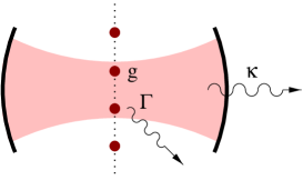
Figure 1: Experimental setup for the preparation of arbitrary entangled states. The system consists of two two-level atoms which can be moved in and out of an optical leaky cavity. An atom inside the cavity couples to the cavity mode with coupling strength $g$. A photon leaks out through the cavity mirrors with a rate $\kappa$ and $\Gamma$ is the spontaneous decay rate of each atom.

II.1 The preparation of an entangled state of two atoms

To explain the main idea of the entanglement scheme we consider first only two two-level atoms with the states $|0\rangle$ and $|1\rangle$ which are in resonance with the cavity mode, $\omega_{\rm cav}=\omega_{0}$, and describe the preparation of the entangled state

$$|\varphi\rangle = \alpha\,|a\rangle+\sqrt{1-|\alpha|^{2}}\,|00\rangle~{},$$ (1)

where

$$|a\rangle \equiv \big{(}|10\rangle-|01\rangle\big{)}/\sqrt{2}$$ (2)

is a maximally entangled state of the two atoms and $\alpha$ an arbitrary parameter. To do so the two atoms, initially in the ground state, $|\psi_{0}\rangle=|00\rangle$, have to be moved into the cavity which should be empty. In addition, a single laser pulse of length $T$, which is in resonance with the atoms, $\omega_{\rm laser}=\omega_{0}$, has to be applied. This laser couples with a Rabi frequency $\Omega^{(i)}$ to atom and we define

$$\Omega^{(-)} \equiv \big{(}\Omega^{(1)}-\Omega^{(2)}\big{)}/\sqrt{2}~{}.$$ (3)

There are two sources of decoherence in the system: spontaneous emission by each atom with rate $\Gamma$ and leakage of photons through the cavity mirrors with rate $\kappa$. We assume here that the later one is the main source for dissipation and a strong coupling between the atoms and the cavity mode, i.e.

$$\Gamma\ll|\Omega^{(-)}|\ll g^{2}/\kappa~{}{\rm and}~{}\kappa~{}.$$ (4)

For this parameter regime, one can show that the state of the atoms at the end of the pulse is given by Eq. (1) with

$$\alpha = -{\rm i}\,{\Omega^{(-)}\over|\Omega^{(-)}|}\,\sin\left({|\Omega^{(-)}|T\over 2}\right)~{}.$$ (5)

To do so we now have a closer look at the time evolution of the system.

To describe the time evolution of the system we make use of the quantum jump approach HeWi1 ; HeWi2 ; HeWi3 . It predicts that the (unnormalized) state of a quantum mechanical system under the condition of no photon emission equals at time $t$

$$|\psi^{0}(t)\rangle = \exp\left(-{{\rm i}\over\hbar}H_{\rm cond}t\right)|\psi_{0}\rangle$$ (6)

where the conditional Hamiltonian $H_{\rm cond}$ is a non-Hermitian Hamiltonian. For the total system consisting of the two atoms and the cavity mode it is given by

$$H_{\rm cond} = {\rm i}\hbar g\,\sum_{i=1}^{2}\big{(}b\,|2\rangle_{ii}\langle 0|-{\rm h.c.}\big{)}$$ (7)

$$+{\hbar\over 2}\sum_{i=1}^{2}\big{(}\,\Omega^{(i)}\,|2\rangle_{ii}\langle 0|+{\rm h.c.}\,\big{)}$$

$$-{\rm i}\hbar\Gamma\sum_{i=1}^{2}|2\rangle_{ii}\langle 2|-{\rm i}\hbar\kappa\,b^{\dagger}b~{},$$

where $b$ is the annihilation operator for a single photon in the cavity mode. As a consequence of the non-Hermitian terms in Eq. (7), the norm of the state vector $|\psi^{0}(t)\rangle$ decreases with time and its squared norm at time $t$ gives the probability for no photon emission in $(0,t)$, i.e.

$$P_{0}(t) = \|\,|\psi^{0}(t)\rangle\,\|^{2}.$$ (8)

For the parameter choice (4) we can show that this probability is very close to unity, which is why we have to consider only the no-photon time evolution of the system.

Because of Eq. (4), there are two very different time scales in the system. One can therefore solve the conditional time evolution of the system with the help of an adiabatic elimination of the fast varying states. This has been done in Ref. ent . Alternatively one can solve Eq. (6) numerically. Here we only present numerical results. Fig. 2 shows the probability for no photon emission obtained from a numerical integration of Eq. (6). As an example we choose the preparation of the maximally entangled state $|a\rangle$ with $T=\pi/|\Omega^{(-)}|$. If a photon is emitted in $(0,T)$ the preparation failed and has to be repeated. Nevertheless, as Fig. 2 shows, the success rate of the scheme is very close to unity. The fidelity of the state $|\psi^{0}(T)\rangle$ in case of a successful preparation is found to be always higher than $95\,\%$ for the parameters chosen in Fig. 2.

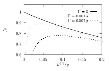
Figure 2: The probability for no photon emission during the preparation of the maximally entangled state $|a\rangle$ for different Rabi frequencies $\Omega^{(1)}$ and $\Omega^{(1)}=-\Omega^{(2)}$, different spontaneous decay rates $\Gamma$ and $\kappa=g$.

The main limiting factor of the scheme is spontaneous emission by the atoms with rate $\Gamma$. To suppress this one can make use of an additional atomic level 2. As described in detail in Ref. Bell , this level should form together with the levels 0 and 1 a $\Lambda$ configuration. Choosing the parameters as in Ref. Bell , level 2 can be eliminated adiabatically, which leads to atomic two-level systems as described above. But now the states $|0\rangle$ and $|1\rangle$ are stable ground states and do not decay.

We now want to give a more intuitive explanation why the scheme works. It takes advantage of the fact that two-level atoms inside the cavity possess decoherence-free states ent ; DFS1 ; DFS2 ; DFS3 . Decoherence-free states arise if no interaction between the system and its environment of free radiation fields takes place. If we neglect spontaneous emissions this is exactly the case if the cavity mode is empty ent . In addition, the systems own time evolution due to the interaction between the atoms and the cavity mode should not lead to the population of non decoherence-free states. From this condition we find that the decoherence-free states are the superpositions of the two atomic states $|00\rangle$ and $|a\rangle$ while the cavity mode is empty. Eq. (1) corresponds therefore to the decoherence-free states of the system.

How the preparation scheme works can now easily be understood in terms of an environment induced quantum Zeno effect misra ; Itano ; zeno . Let us define $\Delta T$ as the time in which a photon leaks out through the cavity mirrors with a probability very close to unity if the system is initially prepared in a state with no overlap with a decoherence-free state. On the other hand, a system in a decoherence-free state will definitely not emit a photon in $\Delta T$. Therefore the observation of the free radiation field over a time interval $\Delta T$ can be interpreted as a measurement of whether the system is decoherence-free or not messung . The outcome of the measurement is indicated by an emission or no emission of a photon. As it has been shown in Ref. messung , $\Delta T$ is of the order $1/\kappa$ and $\kappa/g^{2}$ and much smaller than the typical time scale for the laser interaction.

Here the system continuously interacts with its environment and the system behaves like a system under continuous observation. Therefore, the quantum Zeno effect predicts that all transitions to non decoherence-free states are strongly inhibited. Nevertheless, there is no inhibition of transitions between decoherence-free states and the effect of the laser field on the atomic states can be described by the effective Hamiltonian ent

$$H_{\rm eff} = I\!\!P_{\rm DFS}\,H_{\rm cond}\,I\!\!P_{\rm DFS}~{},$$ (9)

where $I\!\!P_{\rm DFS}$ is the projector on the decoherence-free subspace. If we neglect spontaneous emission Eq. (7) leads to

$$H_{\rm eff}^{\rm(atoms)} = {\hbar\Omega^{(-)}\over 2}\,|a\rangle\langle 00|+{\rm h.c.}$$ (10)

for the atoms, while the cavity remains empty. By solving the corresponding time evolution, one finds that a laser pulse of length $T$ prepares the atoms indeed in state (1) with $\alpha$ given by Eq. (5). Varying the length of the laser pulse allows to change arbitrarily the amount of entanglement of the prepared state.

II.2 Generalization to $N$ atoms and arbitrary entangled states

The entanglement scheme described in the previous subsection allows only for the preparation of certain entangled states of two atoms Bell . For many applications, however, one has to be able to prepare arbitrary entangled states of $N$ two-level atoms with $N\geq 2$. In this subsection we show how this can be done by generalizing the scheme described above.

One possibility to increase the number of decoherence-free states in the system is to move $N$ two-level atoms simultaneously into the cavity. This has been discussed in Ref. ent where the decoherence-free states of this system have been constructed explicitly. However, for applications like quantum computing it is crucial to have simple qubits. Ideally, the logical qubits should be the same as the physical qubits. This can be achieved by using three-level atoms with a $\Lambda$ configuration as shown in Fig. 3. In the following, each qubit is obtained from the ground states $|0\rangle$ and $|1\rangle$ of one atom which are the ground states in the $\Lambda$ configuration.

Figure 3: Each qubit is obtained from the ground states $|0\rangle$ and $|1\rangle$ of one atom. To entangle the atoms an additional level 2 is used which is only populated during a gate operation. The 1-2 transition is in resonance with the cavity mode and couples to the cavity field with a coupling strength $g$. The spontaneous decay rate of level 2 is denoted by $\Gamma$.

The setup we use is the same as shown above in Fig. 1. We assume again that the atoms are trapped in a way that two of them can be moved simultaneously into the cavity. As shown in Fig. 3, the 1-2 transition is in resonance with the cavity field, while the 0-2 transition is highly detuned and we denote the coupling constant of each atom to the cavity mode again by $g$. The spontaneous decay rate of level 2 is given by $\Gamma$. Note, that the system is, in principle, scalable. Arbitrary many atoms can be used.

To prove that it is possible to prepare arbitrary states of the atoms we only have to show that it is possible to perform universal quantum gates between all qubits Vinc . The pair of operations we choose here and discuss in some detail in the next two subsections are the same as discussed in Ref. Tregenna : the single qubit rotation and the CNOT operation. Both gates can be realized with the help of a single laser pulse.

The single qubit rotation. The single qubit rotation is defined by the single atom operator

$$U_{\rm SQR}(\xi,\phi)\equiv\cos\xi-{\rm i}\sin\xi\left({\rm e}^{{\rm i}\phi}|0\rangle\langle 1|+{\rm h.c.}\right)~{}.$$ (11)

To perform this operation one can make use of an adiabatic population transfer Vit — a technique which has been realized in many experiments pop . In order to do this, the atom has to be moved out of the cavity. Then two lasers, both with the same detuning, are applied simultaneously. One couples to the 1-2 transition and the other two the 0-1 transition, both with the same Rabi frequencies. A detailed description of this process can be found in Refs. Bell ; Tregenna .

The CNOT gate. A CNOT operation changes the state of the target atom, which we call in the following atom 2, conditional on the state of the control atom, atom 1, being in $|1\rangle$. It can be described by the operator

$$U_{\rm CNOT} \equiv |10\rangle\langle 11|+|11\rangle\langle 10|~{}.$$ (12)

To perform this gate operation both atoms have to be moved into the cavity and two laser fields are applied simultaneously. One of the lasers couples with the Rabi frequency $\Omega_{1}^{(1)}$ to the 1-2 transition in atom 1, while the other excites the 0-2 transition of atom 2 with the Rabi frequency $\Omega_{0}^{(2)}$. In the following we assume

$$\Omega_{1}^{(1)}=\Omega_{2}^{(0)}\equiv\sqrt{2}\,\Omega$$ (13)

and

$$\Gamma\ll|\Omega|\ll g^{2}/\kappa~{} {\rm and} ~{}\kappa~{}.$$ (14)

Then, as above, spontaneous emission by the atoms during the gate operation can be neglected. In addition, it can be shown that in this parameter regime non decoherence-free states lead to photon emissions on a time scale much smaller than the typical time scale for the laser interaction. As shown in Refs. Tregenna ; Tregenna2 , the effect of the laser fields over a time

$$T = \sqrt{2}\pi/|\Omega|$$ (15)

assembles the CNOT operation to a very good approximation.

To understand why this is the case let us first discuss what the decoherence-free states of the system are. If we consider only the two atoms inside the cavity and apply the same criteria as above we find that the decoherence-free states of the system are the superpositions of the states $|00\rangle$, $|01\rangle$, $|10\rangle$, $|11\rangle$, which form the qubits, and

$$|a\rangle \equiv \big{(}|12\rangle-|21\rangle\big{)}/\sqrt{2}$$ (16)

if one sets $\Omega\equiv 0$ and $\Gamma\equiv 0$. At the same time the cavity has to be empty.

The additional decoherence-free state (16) is a maximally entangled state of the two atoms inside the cavity. Populating this state can therefore be used to create entanglement. To make sure that the laser pulse does not populate other states than the decoherence-free ones the scheme utilizes as above the environment induced quantum Zeno effect Tregenna .

The conditional Hamiltonian of the two atoms inside the cavity equals here Tregenna2

$$H_{\rm cond} = {\rm i}\hbar g\sum_{i}\big{(}b\,|2\rangle_{ii}\langle 1|-{\rm h.c.}\big{)}$$ (17)

$$+{1\over 2}\,\sqrt{2}\,\hbar\Omega\,\big{(}|0\rangle_{22}\langle 2|+|1\rangle_{11}\langle 2|+{\rm h.c.}\big{)}$$

$$-{\rm i}\hbar\kappa\,b^{\dagger}b-{\rm i}\hbar\Gamma\sum_{i}|2\rangle_{ii}\langle 2|~{}.$$

Using Eq. (9) this leads to the effective Hamiltonian

$$H^{(\rm atoms)}_{\rm eff} = {\hbar\Omega\over 2}\,\big{(}|10\rangle\langle a|-|a\rangle\langle 11|+{\rm h.c.}\big{)}$$ (18)

for the atoms, while the cavity remains again empty during the gate operation. By solving the corresponding time evolution of this Hamiltonian one can show that a laser pulse of length $T$ as in Eq. (15) leads indeed to the realization of a CNOT gate.

Finally we conclude with some numerical results. Fig. 4 results from a numerical integration of the time evolution given by Eq. (17) and shows the success rate of a single gate operation for different parameters and the initial state $|10\rangle$.

Figure 4: The probability for no photon emission during a CNOT operation as a function of the Rabi frequency $\Omega$, $\kappa=g$, different spontaneous decay rates $\Gamma$ and the initial state $|10\rangle$.

Fig. 5 shows the fidelity of the prepared state. As in the previous subsection, the fidelity of the scheme in case of no photon emission is very high. Problems arise again from the presence of spontaneous emission, but again this can be suppressed as well by making use of additional levels Tregenna2 .

Figure 5: The fidelity for a single CNOT operation as a function of the Rabi frequency $\Omega$, $\kappa=g$, different spontaneous decay rates $\Gamma$ and initial state $|10\rangle$.

III Entangling atoms inside a Photonic crystal

In this section we give a short overview over another recent scheme by Angelakis et al. Angelakis01 to prepare two atoms in an entangled state using a photonic crystal (or photonic band gap material-PG). The experimental setup of this scheme is shown in Fig. 6 and the entanglement between the atoms originates from the interaction of two atoms with a resonant defect mode.

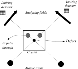
Figure 6: Experimental setup of the proposed PBG atom entanglement scheme.

The first atom is prepared in the upper of two optically separated states, denoted in the following by $|e_{1}\rangle$ and propagates into the transition in the PBG. This atom is unable to emit a photon Angelakis01 due to the exclusion of electromagnetic modes over a continuous range of frequencies Yablonovitch87 and hence a long lived photon-atom bound state of the form John91 ; Lin99

$$|\Psi\rangle = c_{e}(t_{1})\,|e_{1}\rangle|0\rangle+c_{g}(t_{1})\,|g_{1}\rangle|1\rangle,$$ (19)

is formed, where $t_{1}$ is the interaction time of atom 1 with the defect and $|g_{1}\rangle$ the ground state of the atom. The coefficients $c_{e}(t_{1})$ and $c_{g}(t_{1})$ can be derived using a Jaynes-Cummings Hamiltonian. As soon as atom 1 leaves the defect region, a second atom, atom 2, prepared in its ground state $|g_{2}\rangle$ is send through. If $t_{2}$ is the interaction time of this atom with the defect, then the final state of the system is of the form

$$|\Psi_{f}\rangle = c_{e}(t_{1})\,|e_{1}\rangle|g_{2}\rangle|0\rangle+c_{g}(t_{1})c_{e}(t_{2})\,|g_{1}\rangle|g_{2}\rangle|1\rangle$$ (20)

$$+c_{g}(t_{1})c_{g}(t_{2})\,|g_{1}\rangle|e_{2}\rangle|0\rangle$$

With an appropriate choice of $t_{1}$ and $t_{2}$ (for details see Ref. Angelakis01 ) one can achieve that the prepared states equals

$$|\Psi_{f}\rangle = {1\over\sqrt{2}}\,\big{(}|e_{1}\rangle|g_{2}\rangle+|g_{1}\rangle|e_{2}\rangle\big{)}\otimes|0\rangle$$ (21)

which is a maximally entangled state of the two atoms.

IV Entanglement Verification

One of the main problems with entanglement schemes using the no-photon time evolution of a system is, that someone who performs the experiment cannot know for sure whether the scheme worked or not. Measuring whether no photon has been emitted during the whole experiment would require perfect photon detectors which cover all solid angels. It is therefore crucial to have other tests whether a preparation schemes succeeds or not.

What one can do is to use the scheme to prepare a certain maximally entangled state of the atoms and to verify it by observing a violation of a Bell inequality. In this section we describe how to observe a violation of a Bell’s inequality for two atoms and Mermin’s GHZ inequality mermin for multiple atoms. It is important to note that for each pure two qubit state, there exists always a Bell inequality which can be violated.

To do so one has to be able to measure whether an atom is in state $|0\rangle$ or $|1\rangle$ with a very high precision. This can be done following a proposal by Cook Cook . A detailed analysis of this measurement scheme can be found in Ref. behe .

IV.1 A test for two atoms

Given that the state (1) can be generated, the next interesting question is whether it violates one of Bell’s inequalities? For certain parameters it must but what physical measurements are necessary?

The spin (or correlation function) Bell inequality Bell65 ; CHSH69 may be written formally as

$$B_{\rm S} = |E\left(\theta_{1},\theta_{2}\right)-E\left(\theta_{1},\theta_{2}^{\prime}\right)$$ (22)

$$+E\left(\theta_{1}^{\prime},\theta_{2}\right)+E\left(\theta_{1}^{\prime},\theta_{2}^{\prime}\right)|\leq 2~{},$$

where the correlation function $E\left(\theta_{1},\theta_{2}\right)$ is given by

$$E\left(\theta_{1},\theta_{2}\right) = \langle\sigma^{(1)}_{\theta_{1}}\sigma^{(2)}_{\theta_{2}}\rangle~{}.$$ (23)

Here $\theta_{1}$ and $\theta_{2}$ are real parameters. In the following the operator $\sigma_{a}^{(i)}$ with $a=x$, $y$ or $z$ is the $a$ Pauli spin operators for the two-level system of atom $i$ and the operator $\sigma^{(i)}_{\theta_{i}}$ is defined as

$$\sigma^{(i)}_{\theta_{i}}\equiv\cos\theta_{i}\,\sigma^{(i)}_{x}+\sin\theta_{i}\,\sigma^{(i)}_{y}~{}.$$ (24)

For the state considered here the correlation function depends only on the difference between the angles $\theta_{1}$ and $\theta_{2}$ and we have $E\left(\theta_{1},\theta_{2}\right)=E\left(\theta_{1}-\theta_{2},0\right)$. Now if we choose $\vartheta=\theta_{1}-\theta_{2}=\theta_{2}-\theta_{1}^{\prime}=\theta_{1}^{\prime}-\theta_{2}^{\prime}$ and $\theta_{1}-\theta_{2}^{\prime}=3\vartheta$ the inequality (22) simplifies to

$$B_{\rm S}=|3E\left(\vartheta,0\right)-E\left(3\vartheta,0\right)|\leq 2$$ (25)

and a violation of this inequality corresponds to $|B_{\rm{S}}|>2$.

It is straightforward to show that the correlation function for the entangled state (1) is given by

$$E\left(\vartheta,0\right)=-|\alpha|^{2}\cos\vartheta$$ (26)

and hence Eq. (25) can assume a maximum of $|B_{\rm S}|=2\sqrt{2}\,|\alpha|^{2}$ for $\vartheta=\pi/4$. Therefore, a violation of the spin Bell inequality is possible for $|\alpha|^{2}>1/\sqrt{2}$ given our analyzer choices. How $|\alpha|^{2}$ can be expressed in terms of the system parameter $|\Omega^{(-)}|T$ is shown in Eq. (5). In Fig. (7) we plot $|B_{\rm S}|$ versus $|\Omega^{(-)}|T$ and $\vartheta$.

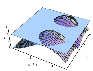
Figure 7: Plot of $|B_{\rm S}|$ versus $|\Omega^{(-)}|T$ and $\vartheta$. A violation of the spin Bell’s inequality occurs for $|B_{\rm S}|>2$ and are displayed as Islands in the $|\Omega^{(-)}|T$ - $\vartheta$ plane. The angles have been chosen so as to maximize the violation utilizing the maximally entangled state.

A significant region of violation is observed with the maximum of $|B_{\rm S}|=2\sqrt{2}$ occurring at $|\Omega^{(-)}|T=\pi$. The state of the atoms at such a time is a maximally entangled state $|a\rangle$. This test on Bell’s inequality can therefore be used to verify the preparation of this state with a high precision and should be feasible with current technology.

IV.2 A Test for multiple atoms

So far, we have discussed how our preparation method can be tested for two atoms. A similar procedure can be used for multiple atoms depending on the state prepared. For instance in the case of three atoms we could prepare a state of the form

$$|\Psi\rangle={1\over\sqrt{2}}\,\big{(}|0\rangle|0\rangle|0\rangle+|1\rangle|1\rangle|1\rangle\big{)}~{}.$$ (27)

This state is known as the GHZ state GHZ . To characterize it we now use Mermin GHZ inequality mermin instead of a Bell inequality. This inequality has the form

$$F = \left|\langle\sigma_{x_{1}}\sigma_{x_{2}}\right.\sigma_{x_{3}}\rangle-\langle\sigma_{y_{1}}S\sigma_{y_{2}}\sigma_{x_{3}}\rangle$$ (28)

$$-\left.\langle\sigma_{y_{1}}\sigma_{x_{2}}\sigma_{y_{3}}\rangle-\langle\sigma_{x_{1}}\sigma_{y_{2}}\sigma_{y_{3}}\rangle\right|\leq 2.$$

For the state (27) we can calculate the moments $\langle\sigma_{x_{1}}\sigma_{x_{2}}\sigma_{x_{3}}\rangle$, $\langle\sigma_{y_{1}}S\sigma_{y_{2}}\sigma_{x_{3}}\rangle$, $\langle\sigma_{y_{1}}\sigma_{x_{2}}\sigma_{y_{3}}\rangle$ and $\langle\sigma_{x_{1}}\sigma_{y_{2}}\sigma_{y_{3}}\rangle$ using a similar procedure to that discussed in the Bell test. We find that $F=4$ for the state (27) while the maximum according to local realism is $F=2$. For entangled states of more atoms ($N>3$) a generalized form of Mermin’s inequality can be employed.

V Discussion

In this proceeding we used the recent results of Refs. ent ; Tregenna and described a scheme to prepare arbitrary entangled states of $N$ atoms in a controlled way with a very high success rate. The scheme is based on the existence of decoherence-free states and an environment induced quantum Zeno effect to avoid the population of non decoherence-free states during the preparation. In addition, we gave a short overview over a recently proposed scheme by Angelakis et al. Angelakis01 to entangle two atoms inside a photonic crystal.

During the state preparation no photons are emitted and observing a violation of Bell’s inequality is one of the ways to test whether the scheme has worked with a high precision or not. We describe the possible violation of Bell’s inequality for two atoms. An entangled state of $N$ two-level atoms can characterized and verified similarly with Mermin’s inequality.

Acknowledgments. We acknowledge the support of the UK Engineering and Physical Sciences Research Council and the European Union and D. G. A. acknowledges the support by the Greek State Scholarship Foundation.

References

- (1) C. H. Bennett, Physics Today, 24 (Oct. 1995); A. Zeilinger, Physics World 11, 09 (1998).
- (2) D. P. DiVincenzo, quant-ph/0002077.
- (3) S. F. Huelga, C. Macchiavello, T. Pellizzari, A. Ekert, M. B. Plenio, and J. I. Cirac, Phys. Rev. Lett. 79, 3865 (1997)
- (4) A. Einstein, B. Podolsky, and N. Rosen, Phys. Rev. 47, 777 (1935).
- (5) J. S. Bell, Physics (N.Y.) 1, 195 (1965).
- (6) J. F. Clauser and M. A. Horne, Phys. Rev. D 10, 526 (1974).
- (7) J. F. Clauser, M. A. Horne, A. Shimony, and R. A. Holt, Phys. Rev. Lett. 23, 880 (1969).
- (8) S. L. Braunstein and C. M. Caves, Phys. Rev. Lett. 61, 622 (1988).
- (9) A. Aspect, P. Grangier, and G. Roger, Phys. Rev. Lett. 49, 91 (1982).
- (10) P. G. Kwiat, K. Mattle, H. Weinfurter, and A. Zeilinger, Phys. Rev. Lett. 75, 4337 (1995).
- (11) W. Tittel, J. Brendel, H. Zbinden, and N. Gisin, Phys. Rev. Lett. 17, 3563 (1998).
- (12) M. A. Rowe, D. Kielpinski, V. Meyer, C. A. Sackett, W. M. Itano, C. Monroe, and D. J. Wineland, Nature 409, 791 (2001).
- (13) R. C. Cook, Physica Scr. T21, 49 (1998).
- (14) A. Beige and G. C. Hegerfeldt, J. Mod. Phys. 44, 345 (1997).
- (15) G. M. Palma, K. A. Suominen, and A. K. Ekert, Proc. Roy. Soc. London Ser. A 452, 567 (1996).
- (16) P. Zanardi and M. Rasetti, Phys. Rev. Lett. 79, 3306 (1997).
- (17) D. A. Lidar, I. L. Chuang, and K. B. Whaley, Phys. Rev. Lett. 81, 2594 (1998).
- (18) L. M. Duan and G. C. Guo, Phys. Rev. A 58, 3491 (1998).
- (19) A. Beige, D. Braun, and P. L. Knight, New J. Phys. 2, 22 (2000).
- (20) A. Beige, D. Braun, B. Tregenna, and P. L. Knight, Phys. Rev. Lett. 85, 1762 (2000).
- (21) D. Bacon, J. Kempe, D. A. Lidar, and K. B. Whaley, Phys. Rev. Lett. 85, 1758 (2000).
- (22) J. Reichel, W. Hansell, and T. W. Hänsch, Phys. Rev. Lett. 83, 3398 (1999).
- (23) R. Folman, P. Krüger, D. Cassettari, B. Hessmo, T. Maier, and J. Schmiedmayer, Phys. Rev. Lett. 84, 4749 (2000).
- (24) G. C. Hegerfeldt and T. S. Wilser, in Classical and Quantum Systems, Proceedings of the Second International Wigner Symposium, July 1991, edited by H. D. Doebner, W. Scherer, and F. Schroeck (World Scientific, Singapore, 1992), p. 104.
- (25) J. Dalibard, Y. Castin, and K. Mølmer, Phys. Rev. Lett. 68, 580 (1992).
- (26) H. Carmichael, An Open Systems Approach to Quantum Optics, Lecture Notes in Physics, Vol. 18 (Springer, Berlin, 1993).
- (27) A. Beige, W. J. Munro, and P. L. Knight, Phys. Rev. A 62, 052102 (2000).
- (28) B. Misra and E. C. G. Sudarshan, J. Math. Phys. 18, 756 (1977).
- (29) W. M. Itano, D. J. Heinzen, J. J. Bollinger, and D. J. Wineland, Phys. Rev. A 41, 2295 (1990).
- (30) A. Beige and G. C. Hegerfeldt, Phys. Rev. A 53, 53 (1996).
- (31) A. Beige, S. Bose, D. Braun, S. F. Huelga, P. L. Knight, M. B. Plenio, and V. Vedral, J. Mod. Opt. 47, 2583 (2000).
- (32) N. V. Vitanov and S. Stenholm, Phys. Rev. A 55, 648 (1997).
- (33) K. Bergmann, H. Heuer, and B. W. Shore, Rev. Mod. Phys. 70, 1003 (1998).
- (34) B. Tregenna, A. Beige, and P. L. Knight (in preparation).
- (35) D. G. Angelakis, E. Paspalakis, and P. L. Knight, Phys. Rev. A 61, 055802 (2000); E. Paspalakis, D. G. Angelakis, and P. L. Knight, Opt. Comm. 172, 229 (1999); D. G. Angelakis, E. Paspalakis, and P. L. Knight, quant-ph0009106.
- (36) E. Yablonovitch, Phys. Rev. Lett 58, 2059 (1987); S. John, Phys. Rev. Lett. 53, 2169 (1984).
- (37) S. John and J. Wang, Phys. Rev B 43, 12 772 (1991).
- (38) S.-Y. Lin and J. G. Fleming, Phys. Rev. B 59, R15579 (1999).
- (39) N. D. Mermin, Phys. Rev. Lett. 65, 1838 (1990).
- (40) D. M. Greenberger, M. A. Horne, and A. Zeilinger, Bell’s Theorem, Quantum Theory and Conceptions of the Universe, edited by M. Kafatos (Kluwer Academic, Dordrecht, 1989) p.73; D. M. Greenberger, M. A. Horne, A. Shimony, and A. Zeilinger, Am. J. Phys. 58, 1131 (1990).