3D input-output relations of quantized light
at dispersing and absorbing multilayer dielectric plates

Abstract

The theory developed by Gruner and Welsch [Phys. Rev. A 54, 1661 (1996)] for calculating the 1D input-output relations of the quantized electromagnetic field at dispersing and absorbing dielectric (multilayer) plates is generalized to the three-dimensional case. First a general recipe for the derivation of the reflection and transmission coefficients at an arbitrary body that separates two half spaces from each other is presented. The general theory is then applied to the case of planar multilayer structures, for which the Green tensor is well-known.

I Introduction

Dielectric bodies such as beam splitters are vital ingredients in quantum-optical experiments. Their properties are of utmost importance for experiments with nonclassical light. For example, losses due to absorption are known to degrade entanglement [1]. The action on light of macroscopic bodies is commonly described in terms of input-output relations. Recently, the 1D input-output relations of the quantized electromagnetic field at a multilayer dielectric plate [2] have been used for constructing CP maps for light interacting with a dispersing and absorbing beam splitter [1, 3].

In the present article we generalize the formalism given in [2] and derive the 3D input-output relations of the quantized electromagnetic field at a dispersing and absorbing multilayer dielectric plate. The theory is essentially based on the quantization of the macroscopic Maxwell field in dispersing and absorbing dielectrics (for a review on this topic, see Ref. [4]) where absorption is taken into account by introducing (for each frequency $\omega$) a bosonic operator noise current density which in turn is related to some fundamental (collective) bosonic excitations of the electromagnetic field and the dielectric matter as

$$\hat{\bf j}({\bf r},\omega)=\omega\sqrt{\frac{\hbar\epsilon_{0}}{\pi}\,\epsilon^{\prime\prime}({\bf r},\omega)}\,\hat{\bf f}({\bf r},\omega),$$ (1)

with $\epsilon^{\prime\prime}({\bf r},\omega)$ being the imaginary part of the complex permittivity function $\epsilon({\bf r},\omega)$]. Solving the corresponding inhomogeneous Helmholtz equation for the electric-field operator in terms of the classical Green tensor ${\sf G}({\bf r},{\bf s},\omega)$, one obtains

$$\hat{\bf E}({\bf r},\omega)=i\omega\mu_{0}\int d^{3}{\bf s}\,{\sf G}({\bf r},{\bf s},\omega)\,\hat{\bf j}({\bf s},\omega)$$ (2)

as the representation of the (Schrödinger-) operator of the electric-field strength in the frequency domain.

Let us assume that the (classical) Green tensor of the electromagnetic field in the presence of the dielectric body under study is known. The input-output relations can then be derived by identifying the contributions to the electromagnetic field in the two half spaces with the input and output fields and the (noise) field produced by the absorbing body. In Section II we give the general recipe, which we specify in Section III for a multilayer dielectric plate.

II Identification of field parts

Let us assume that the space ${\mathbb{R}}^{3}$ can be subdivided into three separated regions I, II, and III, where the region II represents a dielectric body. Although we shall restrict our attention to an infinitely extended plate of thickness $L$, the general results of this section remain also valid for other shapes of the body. Note that the assumption of infinite extension of the plate can be justified by the observation that, typically, the cross-sectional area of an impinging light beam does not exceed the surface area of the plate. 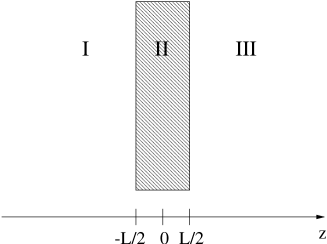For the sake of definiteness, let us denote the regions outside the body with I ($z$ $\!<$ $\!-L/2$) and III ($z$ $\!>$ $\!L/2$) (see Fig. 1).

FIG. 1.: Scheme depicting the dielectric slab located in region II ($-L/2$ $\!\leq$ $\!z$ $\!\leq$ $\!L/2$) surrounded by vacuum in regions I and III.

The electric-field operator (2) in region I is given by

$$\hat{\bf E}^{({\rm I})}({\bf r},\omega)=i\omega\mu_{0}\int_{{\mathbb{R}}^{3}}d^{3}{\bf s}\,{\sf G}^{({\rm I})}({\bf r},{\bf s},\omega)\,\hat{\bf j}({\bf s},\omega),$$ (3)

where the Green tensor can be split into four parts [5]:

$${\sf G}^{({\rm I})}({\bf r},{\bf s},\omega) = {\sf G}^{(10)}({\bf r},{\bf s},\omega)\hskip 9.04166pt\qquad({\bf s}\in{\rm I})$$ (7)

$$+\,{\sf G}^{(11)}({\bf r},{\bf s},\omega)\qquad({\bf s}\in{\rm I})$$

$$+\,{\sf G}^{(12)}({\bf r},{\bf s},\omega)\qquad({\bf s}\in{\rm II})$$

$$+\,{\sf G}^{(13)}({\bf r},{\bf s},\omega)\qquad({\bf s}\in{\rm III}).$$

Here, ${\sf G}^{(10)}({\bf r},{\bf s},\omega)$ is the solution of the inhomogeneous Helmholtz equation (for the case where region I extends the whole space to infinity), and the ${\sf G}^{(1i)}({\bf r},{\bf s},\omega)$ are solutions of the homogeneous Helmholtz equation which insure the correct boundary conditions at the surfaces of discontinuity. The electric-field operator $\hat{\bf E}^{({\rm III})}({\bf r},\omega)$ in region III is given accordingly.

Let us consider the left surface. The identification of the contributions of input and output fields in Eq. (3) [together with Eq. (7)] is unique. The term determined by the free Green tensor ${\sf G}^{(10)}({\bf r},{\bf s},\omega)$ represents the input field. The term determined by ${\sf G}^{(11)}({\bf r},{\bf s},\omega)$ is the contribution of the field which is reflected at the surface, whereas the term determined by ${\sf G}^{(13)}({\bf r},{\bf s},\omega)$ describes the transmitted field through the dielectric body from the right (region III). The reflected and transmitted fields can then be combined to the output field. It is worth noting that, since the Green tensor contains the full information about the allowed electromagnetic-field structure, the output field may also contain surface-guided waves that propagate along the surface. In particular, surface-guided waves can appear if the permittivity of the material satisfies the conditions $\epsilon^{\prime}({\bf s},\omega)$ $\!<$ $\!0$ and $|\epsilon^{\prime}({\bf s},\omega)|$ $\!\ll$ $\!|\epsilon^{\prime\prime}({\bf s},\omega)|$.

From the above, we can subdivide the field at the left surface (notation ${\bf r}|_{z=-L/2}$ $\!\equiv$ $\!{\bf r}^{-}_{\perp}$) into the input field and the output field as

$$\hat{\bf E}_{\rm I}({\bf r}^{-}_{\perp},\omega)=\hat{\underrightarrow{\bf E}}^{({\rm in})}_{\rm I}({\bf r}^{-}_{\perp},\omega)+\hat{\underleftarrow{\bf E}}^{({\rm out})}_{\rm I}({\bf r}^{-}_{\perp},\omega),$$ (8)

with

$$\hat{\underrightarrow{\bf E}}^{({\rm in})}_{\rm I}({\bf r}^{-}_{\perp},\omega)=i\omega\mu_{0}\int_{\rm I}d^{3}{\bf s}\,{\sf G}^{(10)}({\bf r}^{-}_{\perp},{\bf s},\omega)\,\hat{\bf j}({\bf s},\omega),$$ (9)

$$\hat{\underleftarrow{\bf E}}^{({\rm out})}_{\rm I}({\bf r}^{-}_{\perp},\omega)=i\omega\mu_{0}\int_{\rm I}d^{3}{\bf s}\,{\sf G}^{(11)}({\bf r}^{-}_{\perp},{\bf s},\omega)\,\hat{\bf j}({\bf s},\omega)$$ (12)

$$\hskip 43.05542pt+\,i\omega\mu_{0}\int_{\rm II}d^{3}{\bf s}\,{\sf G}^{(12)}({\bf r}^{-}_{\perp},{\bf s},\omega)\,\hat{\bf j}({\bf s},\omega)$$

$$\hskip 43.05542pt+\,i\omega\mu_{0}\int_{\rm III}d^{3}{\bf s}\,{\sf G}^{(13)}({\bf r}^{-}_{\perp},{\bf s},\omega)\,\hat{\bf j}({\bf s},\omega).$$

Analogously, for the field at the right surface (notation ${\bf r}|_{z=L/2}$ $\!\equiv$ $\!{\bf r}^{+}_{\perp}$) we have

$$\hat{\bf E}_{\rm III}({\bf r}^{+}_{\perp},\omega)=\hat{\underleftarrow{\bf E}}^{({\rm in})}_{\rm III}({\bf r}^{+}_{\perp},\omega)+\hat{\underrightarrow{\bf E}}^{({\rm out})}_{\rm III}({\bf r}^{+}_{\perp},\omega),$$ (13)

with

$$\hat{\underleftarrow{\bf E}}^{({\rm in})}_{\rm III}({\bf r}^{+}_{\perp},\omega)=i\omega\mu_{0}\int_{\rm III}d^{3}{\bf s}\,{\sf G}^{(30)}({\bf r}^{+}_{\perp},{\bf s},\omega)\,\hat{\bf j}({\bf s},\omega),$$ (14)

$$\hat{\underrightarrow{\bf E}}^{({\rm out})}_{\rm III}({\bf r}^{+}_{\perp},\omega)=i\omega\mu_{0}\int_{\rm I}d^{3}{\bf s}\,{\sf G}^{(31)}({\bf r}^{+}_{\perp},{\bf s},\omega)\,\hat{\bf j}({\bf s},\omega)$$ (17)

$$\hskip 43.05542pt+\,i\omega\mu_{0}\int_{\rm II}d^{3}{\bf s}\,{\sf G}^{(32)}({\bf r}^{+}_{\perp},{\bf s},\omega)\,\hat{\bf j}({\bf s},\omega)$$

$$\hskip 43.05542pt+\,i\omega\mu_{0}\int_{\rm III}d^{3}{\bf s}{\sf G}^{(33)}({\bf r}^{+}_{\perp},{\bf s},\omega)\,\hat{\bf j}({\bf s},\omega).$$

The arrows indicate the propagation direction of the respective field parts to larger ($\rightarrow$) or smaller ($\leftarrow$) values of $z$. Recall that the output fields may also contain surface-guided waves whose extensions in the directions indicated by the arrows are small.

The first terms in Eqs. (12) and (17) are the reflected fields in the respective regions, the last terms are the transmitted fields from the opposite sides of the body, whereas the second terms arise from sources inside the body. In order to derive the input-output relations, we have to rewrite Eqs. (12) and (17) in terms of the input fields at both sides of the body and noise sources from inside the body. This is always possible in a linear theory considered here, because the superposition principle holds. Thus, we can (formally) write

$$\hat{\underleftarrow{\bf E}}^{({\rm out})}_{\rm I}({\bf r}^{-}_{\perp},\omega)=\int d^{2}{\bf s}^{-}_{\perp}\,{\sf R}_{\rm I}({\bf r}^{-}_{\perp},{\bf s}^{-}_{\perp},\omega)\hat{\underrightarrow{\bf E}}^{({\rm in})}_{\rm I}({\bf s}^{-}_{\perp},\omega)$$ (20)

$$\hskip 25.83325pt+\int d^{2}{\bf s}^{+}_{\perp}\,{\sf T}_{\rm I,III}({\bf r}^{-}_{\perp},{\bf s}^{+}_{\perp},\omega)\hat{\underleftarrow{\bf E}}^{({\rm in})}_{\rm III}({\bf s}^{+}_{\perp},\omega)$$

$$\hskip 25.83325pt+\,\hat{\bf G}_{{\rm I},1}({\bf r}^{-}_{\perp},\omega)+\hat{\bf G}_{{\rm I},2}({\bf r}^{-}_{\perp},\omega),$$

$$\hat{\underrightarrow{\bf E}}^{({\rm out})}_{\rm III}({\bf r}^{+}_{\perp},\omega)=\int d^{2}{\bf s}^{+}_{\perp}\,{\sf R}_{\rm III}({\bf r}^{+}_{\perp},{\bf s}^{+}_{\perp},\omega)\hat{\underleftarrow{\bf E}}^{({\rm in})}_{\rm III}({\bf s}^{+}_{\perp},\omega)$$ (23)

$$\hskip 25.83325pt+\int d^{2}{\bf s}^{-}_{\perp}\,{\sf T}_{\rm III,I}({\bf r}^{+}_{\perp},{\bf s}^{-}_{\perp},\omega)\hat{\underrightarrow{\bf E}}^{({\rm in})}_{\rm I}({\bf s}^{-}_{\perp},\omega)$$

$$\hskip 25.83325pt+\,\hat{\bf G}_{{\rm III},1}({\bf r}^{+}_{\perp},\omega)+\hat{\bf G}_{{\rm III},2}({\bf r}^{+}_{\perp},\omega),$$

with reflection coefficients ${\sf R}$ and transmission coefficients ${\sf T}$ (actually second-rank tensors). The integrations run over the respective surfaces of the body. For example, the field at a point ${\bf r}^{-}_{\perp}$ is created by the input field from the left hitting the surface at points ${\bf s}^{-}_{\perp}$ leading to the first term in Eq. (20), and by the input field from the right hitting the surface at points ${\bf s}^{+}_{\perp}$ thus producing the second term in Eq. (20). As already mentioned, surface-guided modes are generically included in the formalism. The operators $\hat{\bf G}_{{\rm(I,III)},(1,2)}$ are related to the left and right propagating noise excitations inside the body.

The reflection and the transmission coefficients in general depend on the observation point where the field is computed. For example, ${\sf R}_{\rm I}({\bf r}^{-}_{\perp},{\bf s}^{-}_{\perp},\omega)$ obeys the Fredholm integral equation of the first kind

$$\int d^{2}{\bf s}^{-}_{\perp}\,{\sf R}_{\rm I}({\bf r}^{-}_{\perp},{\bf s}^{-}_{\perp},\omega)\,{\sf G}^{(10)}({\bf s}^{-}_{\perp},{\bf s},\omega)\,={\sf G}^{(11)}({\bf r^{-}_{\perp}},{\bf s},\omega),$$ (24)

which has to be inverted to find ${\sf R}_{\rm I}({\bf r}^{-}_{\perp},{\bf s}^{-}_{\perp},\omega)$. Post-multiplying Eq. (24) by $[{\sf G}^{(10)}({\bf s},{\bf x}^{-}_{\perp},\omega)]^{-1}$, integrating over ${\bf s}$, using the relation

$$\int_{\rm I}d^{3}{\bf s}\,{\sf G}^{(10)}({\bf r}^{-}_{\perp},{\bf s},\omega)\left[{\sf G}^{(10)}({\bf s},{\bf x}^{-}_{\perp},\omega)\right]^{-1}=\delta({\bf r}^{-}_{\perp}-{\bf x}^{-}_{\perp}),$$ (25)

and renaming ${\bf x}^{-}_{\perp}$ as ${\bf s}^{-}_{\perp}$, we obtain the reflection coefficient as

$${\sf R}_{\rm I}({\bf r}^{-}_{\perp},{\bf s}^{-}_{\perp},\omega)$$ (27)

$$\hskip 17.22217pt=\int_{\rm I}d^{3}{\bf s}\,{\sf G}^{(11)}({\bf r}^{-}_{\perp},{\bf s},\omega)\left[{\sf G}^{(10)}({\bf s},{\bf s}^{-}_{\perp},\omega)\right]^{-1}.$$

Similarly, the transmission coefficient reads

$${\sf T}_{\rm I,III}({\bf r}^{-}_{\perp},{\bf s}^{+}_{\perp},\omega)$$ (29)

$$\hskip 17.22217pt=\int_{\rm III}d^{3}{\bf s}\,{\sf G}^{(13)}({\bf r}^{-}_{\perp},{\bf s},\omega)\left[{\sf G}^{(30)}({\bf s},{\bf s}^{+}_{\perp},\omega)\right]^{-1}.$$

Analogously, the reflection and transmission coefficients for region III are derived to be

$${\sf R}_{\rm III}({\bf r}^{+}_{\perp},{\bf s}^{+}_{\perp},\omega)$$ (31)

$$\hskip 17.22217pt=\int_{\rm III}d^{3}{\bf s}\,{\sf G}^{(33)}({\bf r}^{+}_{\perp},{\bf s},\omega)\left[{\sf G}^{(30)}({\bf s},{\bf s}^{+}_{\perp},\omega)\right]^{-1},$$

$${\sf T}_{\rm III,I}({\bf r}^{+}_{\perp},{\bf s}^{-}_{\perp},\omega)$$ (33)

$$\hskip 17.22217pt=\int_{\rm I}d^{3}{\bf s}\,{\sf G}^{(31)}({\bf r}^{+}_{\perp},{\bf s},\omega)\left[{\sf G}^{(30)}({\bf s},{\bf s}^{-}_{\perp},\omega)\right]^{-1}.$$

Note, that the reflection and transmission coefficients are polarization-dependent. The remaining task is to invert the free Green tensors ${\sf G}^{(10)}({\bf s},{\bf s}^{\pm}_{\perp},\omega)$ and ${\sf G}^{(30)}({\bf s},{\bf s}^{\pm}_{\perp},\omega)$. This can be done by expanding the inverse Green tensors in terms of a complete set of orthogonal solutions of the Helmholtz equation, i.e. the TE and TM vector potentials, and using their respective orthogonality relations.

III Multilayer dielectric plates

Beam splitters and related (passive) optical elements typically consist of layers with different dielectric properties (for example, anti-reflection coatings). Let us apply the formalism developed in Section II to the calculation of the input-output relations of light at a multilayer dielectric plate. To do so, we have to specify the Green tensor. The Green tensor for planar multilayers can be found in [5, 6, 7] and is presented in the Appendix. All terms contributing to the Green tensor can be given in terms of TE and TM vector potentials thus making the distinction between different polarizations very easy.

Suppose the plate consists of $N$ dielectric layers (hence, region II is subdivided into $N$ subregions II$i$, $i$ $\!=$ $\!1\ldots N$). Then, the input fields are given by Eqs. (9) and (14), and the output fields are given by (12) and (17) with the identifications

$$\int_{\rm II}d^{3}{\bf s}\,{\sf G}^{(12)}({\bf r}^{-}_{\perp},{\bf s},\omega) \equiv \sum\limits_{i=1}^{N}\int_{{\rm II}i}d^{3}{\bf s}\,{\sf G}^{(12i)}({\bf r}^{-}_{\perp},{\bf s},\omega),$$ (34)

$$\int_{\rm II}d^{3}{\bf s}\,{\sf G}^{(32)}({\bf r}^{+}_{\perp},{\bf s},\omega) \equiv \sum\limits_{i=1}^{N}\int_{{\rm II}i}d^{3}{\bf s}\,{\sf G}^{(32i)}({\bf r}^{+}_{\perp},{\bf s},\omega),$$ (35)

leading to the reflection and transmission coefficients according to Eqs. (27) – (33), with the Green tensor being specified in the Appendix. Note, that for planar multilayers different polarizations do not mix, as it can be seen from the structure of the Green tensor, which contains only dyadic products of vector functions of one type. This behaviour is typical of planar layers.

From the Green tensor as given in the Appendix, it is not difficult to identify the noise terms in Eqs. (20) and (23). For propagating waves it is the subdivision into left and right moving waves in the slab. We derive

$$\hat{\bf G}_{{\rm I},1}({\bf r}^{-}_{\perp},\omega)=-\frac{\omega\mu_{0}}{4\pi}\sum\limits_{i=1}^{N}\int\limits_{{\rm II}i}\!d^{3}{\bf s}\int_{0}^{\infty}\!d\lambda\sum\limits_{n=0}^{\infty}\bigg{\{}\frac{2-\delta_{0n}}{\lambda h_{2i}}$$ (38)

$$\hskip 8.61108pt\times\left[A_{M}^{12i}{\bf M}_{{e\atop o}n\lambda}({\bf r}^{-}_{\perp},h_{1}){\bf M}_{{e\atop o}n\lambda}({\bf s},-h_{2i})\right.$$

$$\hskip 8.61108pt\left.+\,A_{N}^{12i}{\bf N}_{{e\atop o}n\lambda}({\bf r}^{-}_{\perp},h_{1}){\bf N}_{{e\atop o}n\lambda}({\bf s},-h_{2i})\right]\,\hat{\bf j}({\bf s},\omega)\bigg{\}},$$

$$\hat{\bf G}_{{\rm I},2}({\bf r}^{-}_{\perp},\omega)=-\frac{\omega\mu_{0}}{4\pi}\sum\limits_{i=1}^{N}\int\limits_{{\rm II}i}\!d^{3}{\bf s}\int_{0}^{\infty}\!d\lambda\sum\limits_{n=0}^{\infty}\bigg{\{}\frac{2-\delta_{0n}}{\lambda h_{2i}}$$ (41)

$$\hskip 8.61108pt\times\left[B_{M}^{12i}{\bf M}_{{e\atop o}n\lambda}({\bf r}^{-}_{\perp},h_{1}){\bf M}_{{e\atop o}n\lambda}({\bf s},h_{2i})\right.$$

$$\hskip 8.61108pt\left.+\,B_{N}^{12i}{\bf N}_{{e\atop o}n\lambda}({\bf r}^{-}_{\perp},h_{1}){\bf N}_{{e\atop o}n\lambda}({\bf s},h_{2i})\right]\,\hat{\bf j}({\bf s},\omega)\bigg{\}},$$

$$\hat{\bf G}_{{\rm III},1}({\bf r}^{+}_{\perp},\omega)=-\frac{\omega\mu_{0}}{4\pi}\sum\limits_{i=1}^{N}\int\limits_{{\rm II}i}\!d^{3}{\bf s}\int_{0}^{\infty}\!d\lambda\sum\limits_{n=0}^{\infty}\bigg{\{}\frac{2-\delta_{0n}}{\lambda h_{2i}}$$ (44)

$$\hskip 8.61108pt\times\left[C_{M}^{32i}{\bf M}_{{e\atop o}n\lambda}({\bf r}^{+}_{\perp},-h_{3}){\bf M}_{{e\atop o}n\lambda}({\bf s},-h_{2i})\right.$$

$$\hskip 8.61108pt\left.+\,C_{N}^{32i}{\bf N}_{{e\atop o}n\lambda}({\bf r}^{+}_{\perp},-h_{3}){\bf N}_{{e\atop o}n\lambda}({\bf s},-h_{2i})\right]\,\hat{\bf j}({\bf s},\omega)\bigg{\}},$$

$$\hat{\bf G}_{{\rm III},2}({\bf r}^{+}_{\perp},\omega)=-\frac{\omega\mu_{0}}{4\pi}\sum\limits_{i=1}^{N}\int\limits_{{\rm II}i}\!d^{3}{\bf s}\int_{0}^{\infty}\!d\lambda\sum\limits_{n=0}^{\infty}\bigg{\{}\frac{2-\delta_{0n}}{\lambda h_{2i}}$$ (47)

$$\hskip 8.61108pt\times\left[D_{M}^{32i}{\bf M}_{{e\atop o}n\lambda}({\bf r}^{+}_{\perp},-h_{3}){\bf M}_{{e\atop o}n\lambda}({\bf s},h_{2i})\right.$$

$$\hskip 8.61108pt\left.+\,D_{N}^{32i}{\bf N}_{{e\atop o}n\lambda}({\bf r}^{+}_{\perp},-h_{3}){\bf N}_{{e\atop o}n\lambda}({\bf s},h_{2i})\right]\,\hat{\bf j}({\bf s},\omega)\bigg{\}}.$$

Let us briefly compare the 3D input-output relations derived here with 1D input-output relations given in [2]. Because of translational invariance along the ($x,y$)-directions and the assumed horizontal incident (propagation along the $z$-axis), the reflection and transmission coefficients in [2] do not depend on spatial coordinates and reduce to scalar functions (of frequency and material parameters). Translational invariance along the ($x,y$)-directions is also assumed in the 3D treatment of the problem, but here the reflection and transmission coefficients must be regarded as space-dependent second-rank tensors in general. Further, the output fields do not only contain volume waves but also surface-guided waves.

IV Conclusions

In this article we have developed a general concept for deriving the 3D input-output relations of optical fields at dispersing and absorbing bodies, and we have applied it to a multilayer dielectric plate. Since the theory is based on the quantization of the electromagnetic field in absorbing media which relies on a source-quantity representation of the field in terms of the (classical) Green tensor, the task reduces to the determination of the Green tensor and its respective contributions to the input and output fields. In this way, the output fields can be related to the input fields via transmission and reflection and to some noise excitation associated with material absorption. Both volume waves and surface-guided waves are included in the input-output relations.

A Green tensor for a dielectric layer

We briefly repeat some basic formulas for the Green tensor in the spectral representation (for details, see [5]). The cylindrical TE and TM vector wave functions for even and odd waves which are frequently used throughout are defined as

$${\bf M}_{{e\atop o}n\lambda}({\bf r},h)=\left[\mp\frac{nJ_{n}(\lambda r)}{r}{\sin\choose\cos}n\psi\,{\bf e}_{r}\right.$$ (A2)

$$\hskip 25.83325pt\left.-\,\frac{dJ_{n}(\lambda r)}{dr}{\cos\choose\sin}n\psi\,{\bf e}_{\psi}\right]e^{ihz},$$

$${\bf N}_{{e\atop o}n\lambda}({\bf r},h)=\frac{1}{k}\left[ih\frac{dJ_{n}(\lambda r)}{dr}{\cos\choose\sin}n\psi\,{\bf e}_{r}\right.$$ (A4)

$$\left.\mp\frac{ihJ_{n}(\lambda r)}{r}{\sin\choose\cos}n\psi\,{\bf e}_{\psi}+\lambda^{2}J_{n}(\lambda r){\cos\choose\sin}n\psi\,{\bf e}_{z}\right]e^{ihz},$$

where $h$ $\!=$ $\!\sqrt{k^{2}-\lambda^{2}}$, $k^{2}$ $\!=$ $\!\epsilon(\omega)(\omega/c)^{2}$, with $\epsilon(\omega)$ being the complex permittivity in the respective region of space.

The Green tensor at source point ${\bf s}$ and field point ${\bf r}$ can always be decomposed into a sum of an (unbounded) free Green tensor ${\sf G}^{(f0)}({\bf r},{\bf s},\omega)$ and the scattering Green tensor ${\sf G}^{(fs)}({\bf r},{\bf s},\omega)$ as

$${\sf G}^{(fs)}({\bf r},{\bf s},\omega)={\sf G}^{(f0)}({\bf r},{\bf s},\omega)\delta_{fs}+{\sf G}^{(fs)}({\bf r},{\bf s},\omega).$$ (A6)

Standard representations of the free Green tensor ${\sf G}^{(f0)}({\bf r},{\bf s},\omega)$ can be found, e.g., in [4, 5, 6, 7]. The scattering Green tensor is given in [5] in the compact form of

$${\sf G}^{(fs)}({\bf r},{\bf s},\omega)=\frac{i}{4\pi}\int_{0}^{\infty}d\lambda\sum\limits_{n=0}^{\infty}\bigg{\{}\frac{2-\delta_{0n}}{\lambda h_{s}}$$ (A19)

$$\hskip 8.61108pt\times\,\bigg{[}(1-\delta_{f3}){\bf M}_{{e\atop o}n\lambda}({\bf r},h_{f})$$

$$\hskip 25.83325pt\times\left[(1\!-\!\delta_{s1})A_{M}^{fs}{\bf M}_{{e\atop o}n\lambda}({\bf s},-h_{s})\right.$$

$$\hskip 51.6665pt\left.+\,(1\!-\!\delta_{s3})B_{M}^{fs}{\bf M}_{{e\atop o}n\lambda}({\bf s},h_{s})\right]$$

$$\hskip 8.61108pt+\,(1-\delta_{f3}){\bf N}_{{e\atop o}n\lambda}({\bf r},h_{f})$$

$$\hskip 25.83325pt\times\left[(1\!-\!\delta_{s1})A_{N}^{fs}{\bf N}_{{e\atop o}n\lambda}({\bf s},-h_{s})\right.$$

$$\hskip 51.6665pt\left.+\,(1\!-\!\delta_{s3})B_{N}^{fs}{\bf N}_{{e\atop o}n\lambda}({\bf s},h_{s})\right]$$

$$\hskip 8.61108pt+\,(1-\delta_{f1}){\bf M}_{{e\atop o}n\lambda}({\bf r},-h_{f})$$

$$\hskip 25.83325pt\times\left[(1\!-\!\delta_{s1})C_{M}^{fs}{\bf M}_{{e\atop o}n\lambda}({\bf s},-h_{s})\right.$$

$$\hskip 51.6665pt\left.+\,(1\!-\!\delta_{s3})D_{M}^{fs}{\bf M}_{{e\atop o}n\lambda}({\bf s},h_{s})\right]$$

$$\hskip 8.61108pt+\,(1-\delta_{f1}){\bf N}_{{e\atop o}n\lambda}({\bf r},-h_{f})$$

$$\hskip 25.83325pt\times\left[(1\!-\!\delta_{s1})C_{N}^{fs}{\bf N}_{{e\atop o}n\lambda}({\bf s},-h_{s})\right.$$

$$\hskip 51.6665pt\left.+\,(1\!-\!\delta_{s3})D_{N}^{fs}{\bf N}_{{e\atop o}n\lambda}({\bf s},h_{s})\right]\bigg{]}\bigg{\}},$$

where the scattering coefficients $A_{M,N}^{fs}$, $B_{M,N}^{fs}$, $C_{M,N}^{fs}$, and $D_{M,N}^{fs}$ are determined by the boundary conditions at the interfaces between the layers. The notation used here is such that the indices of the field and source points cover the range ($1,2i,3$), $i$ $\!=$ $\!1\ldots N$, distinguishing between region I (index $1$), region III (index $3$), and $N$ layers II$i$ (indices $2i$) that build up region II.

REFERENCES

• [1] S. Scheel, L. Knöll, T. Opatrný, and D.-G. Welsch, Phys. Rev. A 62, 043803 (2000).
• [2] T. Gruner and D.-G. Welsch, Phys. Rev. A 54, 1661 (1996).
• [3] L. Knöll, S. Scheel, E. Schmidt, D.-G. Welsch, and A.V. Chizhov, Phys. Rev. A 59, 4716 (1999).
• [4] L. Knöll, S. Scheel, and D.-G. Welsch, QED in dispersing and absorbing dielectric media, to appear in Coherence and Statistics of Photons and Atoms, ed. by J. Peřina, to be published, arXiv: quant-ph/0006121.
• [5] L.W. Li, P.S. Kooi, M.S. Leong, and T.S. Yeo, J. of Electromagn. Waves and Appl. 8, 663 (1994).
• [6] W.C. Chew, Waves and Fields in Inhomogeneous Media (IEEE Press, New York, 1995).
• [7] C.T. Tai, Dyadic Green functions in electromagnetic theory (IEEE Press, New York, 1994).