Possibility of the tunneling time determination

Abstract

We show that it is impossible to determine the time a tunneling particle spends under the barrier. However, it is possible to determine the asymptotic time, i.e., the time the particle spends in a large area including the barrier. We propose a model of time measurements. The model provides a procedure for calculation of the asymptotic tunneling and reflection times. The model also demonstrates the impossibility of determination of the time the tunneling particle spends under the barrier. Examples for $\delta$-form and rectangular barrier illustrate the obtained results.

I Introduction

Tunneling phenomena are inherent in numerous quantum systems, ranging from atom and condensed matter to quantum fields. Therefore, the questions about the tunneling mechanisms are important. There have been many attempts to define a physical time for tunneling processes, since this question has been raised by MacColl [1] in 1932. This question is still the subject of much controversy, since numerous theories contradict each other in their predictions for “the tunneling time”. Some of these theories predict that the tunneling process is faster than light, whereas the others state that it should be subluminal. This subject has been covered in a number of reviews (Hauge and Støvneng [2], 1989; Olkholovsky and Recami [3], 1992; Landauer and Martin [4], 1994 and Chiao and Steinberg [5], 1997). The fact that there is a time related to the tunneling process has been observed experimentally [6, 7, 8, 9, 10, 11, 12, 13, 14]. However, the results of the experiments are ambiguous.

Many of the theoretical approaches can be divided into three categories. First, one can study evolution of the wave packets through the barrier and get the phase time. However, the correctness of the definition of this time is highly questionable [15]. Another approach is based on the determination of a set of dynamic paths, i.e., the calculation of the time the different paths spend in the barrier and averaging over the set of the paths. The paths can be found from the Feynman path integral formalism [16], from the Bohm approach [17, 18, 19, 20], or from the Wigner distribution [21]. The third class uses a physical clock which can be used for determination of the time elapsed during the tunneling (Büttiker and Landauer used an oscillatory barrier [15], Baz’ suggested the Larmor time [22]).

The problems rise also from the fact, that the arrival time of a particle to the definite spatial point is a classical concept. Its quantum counterpart is problematic, even for the free particle case. In classical mechanics for the determination of the time the particle spends moving along a certain trajectory we have to measure the position of the particle at two different moments of time. In quantum mechanics this procedure does not work. From Heisenberg’s uncertainty principle it follows that we cannot measure the position of a particle without alteration of its momentum. To determine exactly the arrival time of a particle, one has to measure the position of the particle with a great precision. Because of the measurement, the momentum of the particle will have a big uncertainty and the second measurement will be indefinite. If we want to ask about the time in quantum mechanics, we need to define the procedure of the measurement. We can measure the position of the particle only with a finite precision and get a distribution of the possible positions. Applying such a measurement, we can expect to obtain not a single value of the traversal time but a distribution of times.

The question How much time does the tunneling particle spend in the barrier region? is not precise. There are two different, but related questions connected with the tunneling time problem [23]:

1. How much time does the tunneling particle spend under the barrier?

2. At what time does the particle arrive to the point behind the barrier?

There have been many attempts to answer these questions. However, there are several papers showing, that according to quantum mechanics the question (i) makes no sense [23, 24, 25, 26]. The goal of this paper is to investigate the possibility to determine the tunneling time using a concrete model of time measurements.

The paper is organized as follows: In section II we prove that it is impossible to determine the time the tunneling particle spends under the barrier. In section III we present the procedure of the time measurement. This procedure leads to the dwell time if no distinctions between tunneled and reflected particles are made. This is shown in section IV. In section V we modify the proposed procedure of the time measurement to make the distinction between tunneled and reflected particles and obtain the tunneling time. The result of such a procedure clearly shows the impossibility of the determination of the tunneling time. However, it also gives the method of the asymptotic time calculation. In sections VI and VII we examine the properties of the tunneling and reflection times. In section VIII, we derive the formula for asymptotic time. Section IX summarizes our findings.

II Impossibility of the tunneling time determination

To answer the question How much time does the tunneling particle spend under the barrier? we need a criterion of the tunneling. In this paper we accept the following criterion: the particle had tunneled in the case it was in front of the barrier at first and later it was found behind the barrier. We require that the mean energy of the particle and the energy uncertainty must be less than the height of the barrier. Following this criterion, we introduce an operator corresponding to the “tunneling-flag” observable. This operator projects the wave function onto the subspace of functions localized behind the barrier

$$\hat{f}_{T}\left(X\right)=\Theta\left(\hat{x}-X\right)$$ (1)

where $\Theta$ is the Heaviside unit step function and $X$ is a point behind the barrier. We call operator $\hat{f}_{T}$ as the tunneling flag operator. This operator has two eigenvalues: $0$ and $1$. The eigenvalue $0$ corresponds to the fact that the particle has not tunneled, while the eigenvalue $1$ corresponds to the tunneled particle.

We will work in the Heisenberg’s representation. In this representation, the tunneling flag operator is

$$\tilde{f}_{T}\left(t,X\right)=\exp\left(\frac{i}{\hbar}\hat{H}t\right)\hat{f}_{T}\left(X\right)\exp\left(-\frac{i}{\hbar}\hat{H}t\right).$$ (2)

To take into account all tunneled particles, the limit $t\rightarrow+\infty$ must be taken. So, the “tunneling-flag” observable in the Heisenberg’s picture is represented by the operator $\tilde{f}_{T}\left(\infty,X\right)=\lim_{t\rightarrow+\infty}\tilde{f}_{T}\left(t,X\right)$. We can obtain explicit expression for this operator.

The operator $\tilde{f}_{T}\left(t,X\right)$ obeys the equation

$$i\hbar\frac{\partial}{\partial\ t}\tilde{f}_{T}\left(t,X\right)=\left[\tilde{f}_{T}\left(t,X\right),\hat{H}\right].$$ (3)

The commutator in Eq. (3) may be expressed as

$\displaystyle\left[\tilde{f}_{T}\left(t,X\right),\hat{H}\right]=\exp\left(\frac{i}{\hbar}\hat{H}t\right)\left[\hat{f}_{T}\left(X\right),\hat{H}\right]\exp\left(-\frac{i}{\hbar}\hat{H}t\right).$

If the Hamiltonian has the form $\hat{H}=\frac{1}{2M}\hat{p}^{2}+V\left(\hat{x}\right)$ then the commutator takes the form

$$\left[\hat{f}_{T}\left(X\right),\hat{H}\right]=i\hbar\hat{J}\left(X\right)$$ (4)

where $\hat{J}\left(X\right)$ is the probability flux operator

$$\hat{J}\left(x\right)=\frac{1}{2M}\left(\left|x\right\rangle\left\langle x\right|\hat{p}+\hat{p}\left|x\right\rangle\left\langle x\right|\right).$$ (5)

Therefore, we have equation for the commutator

$$\left[\tilde{f}_{T}\left(t,X\right),\hat{H}\right]=i\hbar\tilde{J}\left(X,t\right).$$ (6)

The initial condition for the function $\tilde{f\left(t,X\right)}$ may be defined as

$\displaystyle\tilde{f}_{T}\left(t=0,X\right)=\hat{f}_{T}\left(X\right).$

From Eqs. (3) and (6) we obtain equation for the evolution of the tunneling flag operator

$$i\hbar\frac{\partial}{\partial\ t}\tilde{f}_{T}\left(t,X\right)=i\hbar\tilde{J}\left(X,t\right).$$ (7)

From Eq. (7) and initial condition it follows an explicit expression for the tunneling flag operator

$$\tilde{f}_{T}\left(t,X\right)=\hat{f}_{T}\left(X\right)+\int_{0}^{t}dt_{1}\tilde{J}\left(X,t_{1}\right).$$ (8)

In the question “How much time does the tunneling particle spend under the barrier?” we ask about the particles, which we know with certainty have tunneled. In addition, we want to have some information about the location of the particle. However, does quantum mechanics allow us to have the information about the tunneling and location simultaneously? A projection operator

$$\hat{D}\left(\Gamma\right)=\int\limits_{\ \Gamma}dx\left|x\right\rangle\left\langle x\right|$$ (9)

where $\left|x\right\rangle$ is the eigenfunction of the coordinate operator, represents the probability for the particle to be in the region $\Gamma$. In the Heisenberg’s representation this operator takes the form

$$\tilde{D}\left(\Gamma,t\right)=\exp\left(\frac{i}{\hbar}\hat{H}t\right)\hat{D}\left(\Gamma\right)\exp\left(-\frac{i}{\hbar}\hat{H}t\right).$$ (10)

From Eqs. (5), (8) and (10) we see that the operators $\tilde{D}\left(\Gamma,t\right)$ and $\tilde{f}_{T}\left(\infty,X\right)$ in general do not commute. This means that we cannot simultaneously have the information about the tunneling and location of the particle. If we know with certainty that the particle has tunneled then we can say nothing about its location in the past and if we know something about the location of the particle, we cannot determine definitely whether the particle will tunnel. Therefore, the question How much time does the tunneling particle spend under the barrier? cannot be answered in principle, if the question is so posed that its precise definition requires the existence of the joint probability that the particle is found in $\Gamma$ at time $t$ and whether or not it is found on the right side of the barrier at a sufficiently later time. A similar analysis has been performed in Ref. [26]. It has been shown that due to non-commutability of operator there exist no unique decomposition of the dwell time.

This conclusion is, however, not only negative. We know that $\int_{-\infty}^{+\infty}dx\left|x\right\rangle\left\langle x\right|=1$ and $\left[1,\tilde{f}_{T}\left(\infty,X\right)\right]=0$. Therefore, if the region $\Gamma$ is large enough, one has a possibility to answer the question about the tunneling time.

From the fact that the operators $\tilde{D}\left(\Gamma,t\right)$ and $\tilde{f}_{T}\left(\infty,X\right)$ do not commute we can predict that the measurement of the tunneling time will yield a value dependent on the particular detection scheme. The detector is made so that it yields some value. But if we try to measure non-commuting observables, the measured values depends on the interaction between the detector and the measured system. So, in the definition of the Larmor time there is a dependence on the type of boundary attributed to the magnetic-field region [3].

III The model of the time measurement

We consider a model for the tunneling time measurement which is somewhat similar to the “gedanken” experiment used to obtain the Larmor time, but it is simpler and more transparent. This model had been proposed by A. M. Steinberg [27], however, it was treated in non-standard way, introducing complex probabilities. Here we use only the formalism of the standard quantum mechanics.

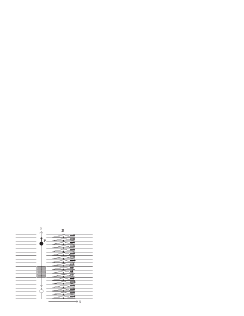
FIG. 1.: The configuration of the measurements of the tunneling time. The particle P is tunneling along $x$ coordinate and it is interacting with detectors D. The barrier is represented by the rectangle. The interaction with the definite detector occurs only in the narrow region limited by the horizontal lines. The changes of the momenta of the detectors are represented by arrows.

Our system consists of particle P and several detectors D. Each detector interacts with the particle only in the narrow region of space. The configuration of the system is shown in Fig. 1. When the interaction of the particle with the detectors is weak the detectors do not influence the state of the particle. Therefore, we can analyze the action of detectors separately.

First of all we consider the interaction of the particle with one detector. The Hamiltonian of the system is

$$\hat{H}=\hat{H}_{P}+\hat{H}_{D}+\hat{H}_{I}$$ (11)

where $\hat{H}_{P}=\frac{1}{2M}\hat{p}^{2}+V\left(\hat{x}\right)$ is the Hamiltonian of the particle, $\hat{H}_{D}$ is the detector’s Hamiltonian and

$$\hat{H}_{I}=\gamma\hat{q}\hat{D}\left(x_{D}\right)$$ (12)

represents the interaction between the particle and the detector. The operator $\hat{q}$ acts in the Hilbert space of the detector. We require a continuous spectrum of the operator $\hat{q}$. For simplicity, we can consider this operator as the coordinate of the detector. The operator $\hat{D}\left(x_{D}\right)$ acts in the Hilbert space of the particle. In the coordinate representation it is nonvanishing only in the small region around the point $x_{D}$. In an ideal case the operator $\hat{D}\left(x_{D}\right)$ may be expressed as $\delta$-function of the particle coordinate,

$$\hat{D}\left(x_{D}\right)\equiv\left|x_{D}\right\rangle\left\langle x_{D}\right|=\delta\left(\hat{x}-x_{D}\right).$$ (13)

Parameter $\gamma$ in Eq. (12) characterizes the strength of the interaction. A very small parameter $\gamma$ ensures the undisturbance of the particle’s motion.

Hamiltonian (12) with $\hat{D}$ given by (13) represents the constant force acting on the detector D when the particle is very close to the point $x_{D}$. This force results in the change of the detector’s momentum. From the classical point of view, the change of the momentum is proportional to the time the particle spends in the region around $x_{D}$ and the coefficient of proportionality equals to the force acting on the detector. In the ordinary quantum mechanics there is no general method of the time determination. If we want to define such a method, we have to make additional assumptions about the time. It is natural to extend the classical method of the time determination into the quantum mechanics, too. Therefore we assume that the change of the mean momentum of the detector is proportional to the time the constant force acts on the detector and that the time the particle spends in the detector’s region is the same as the time the force acts on the detector.

We can replace the $\delta$-function by the narrow rectangle of the width $L$ and height $\frac{1}{L}$. From (12) it follows that the force acting on the detector when the particle is in the region around $x_{D}$ is $-\gamma\frac{1}{L}$. The time the particle spends in the region around $x_{D}$ equals to $\left(-\gamma\frac{1}{L}\right)^{-1}\left(\left\langle p_{q}\left(t\right)\right\rangle-\left\langle p_{q}\right\rangle\right)$ where $p_{q}$ is the momentum of the detector conjugated to the coordinate $q$, while $\left\langle p_{q}\right\rangle$ and $\left\langle p_{q}\left(t\right)\right\rangle$ are the mean initial momentum and momentum after time $t$, respectively. The time the particle spends until time moment $t$ in the unit length region is

$$\tau\left(t\right)=-\frac{1}{\gamma}\left(\left\langle p_{q}\left(t\right)\right\rangle-\left\langle p_{q}\right\rangle\right).$$ (14)

To find the time the particle spends in the region of the finite length, we have to add the times spent in the regions of length $L$. When $L\rightarrow 0$ we obtain an integral.

The evolution operator is

$$\hat{U}\left(t\right)=\exp\left[-\frac{i}{\hbar}\left(\hat{H}_{P}+\hat{H}_{D}+\hat{H}_{I}\right)t\right].$$ (15)

In the moment $t=0$ the density matrix of the whole system is $\hat{\rho}\left(0\right)=\hat{\rho}_{P}\left(0\right)\otimes\hat{\rho}_{D}\left(0\right)$ where $\hat{\rho}_{P}\left(0\right)$ is the density matrix of the particle and $\hat{\rho}_{D}\left(0\right)=\left|\Phi\right\rangle\left\langle\Phi\right|$ is the density matrix of the detector with $\left|\Phi\right\rangle$ being the normalized vector in the Hilbert space of the detector. After the interaction, the density matrix of the detector is $\hat{\rho}_{D}\left(t\right)=Tr_{P}\left\{\hat{U}\left(t\right)\left(\hat{\rho}_{P}\left(0\right)\otimes\left|\Phi\right\rangle\left\langle\Phi\right|\right)\hat{U}^{+}\left(t\right)\right\}$. In the moment $t=0$ it must be $\left\langle\mathstrut x\right|\rho_{P}\left(\mathstrut 0\right)\left|x^{\prime}\right\rangle\neq 0$ only when $x<0$ and $x^{\prime}<0$.

Further, for simplicity we will neglect the Hamiltonian of the detector. The evolution operator then approximately equals to the operator $\hat{U}\left(t,\gamma\hat{q}\right)$ where

$$\hat{U}\left(t,\alpha\right)=\exp\left[-\frac{i}{\hbar}\left(\frac{1}{2M}\hat{p}^{2}+V\left(\hat{x}\right)+\alpha\hat{D}\left(x_{D}\right)\right)t\right].$$ (16)

After such assumptions from our model we can obtain the time, the particle spends in the definite space region. Similar calculations were done for detector’s position rather than momentum by G. Iannaccone [28].

IV Measurement of the dwell time

We expand the operator $\hat{U}\left(t,\gamma\hat{q}\right)$ into the series of the parameter $\gamma$, assuming that $\gamma$ is small. Introducing the operator $\hat{D}\left(x_{D}\right)$ in the interaction representation

$$\tilde{D}\left(x_{D},t\right)=\exp\left(\frac{i}{\hbar}\hat{H}_{P}t\right)\hat{D}\left(x_{D}\right)\exp\left(-\frac{i}{\hbar}\hat{H}_{P}t\right)$$ (17)

we obtain the first order approximation for the operator $\hat{U}\left(t,\gamma\hat{q}\right)$,

$$\hat{U}\left(t,\gamma\hat{q}\right)\approx\exp\left(-\frac{i}{\hbar}\hat{H}_{P}t\right)\left(1+\frac{\gamma\hat{q}}{i\hbar}\int_{0}^{t}dt_{1}\tilde{D}\left(x_{D},t_{1}\right)\right).$$ (18)

For shortening the notation we introduce an operator

$$\hat{F}\left(x_{D},t\right)\equiv\int_{0}^{t}dt_{1}\tilde{D}\left(x_{D},t_{1}\right)$$ (19)

and the equation for the evolution operator $\hat{U}\left(t,\gamma\hat{q}\right)$ is expressed as

$$\hat{U}\left(t,\gamma\hat{q}\right)\approx\exp\left(-\frac{i}{\hbar}\hat{H}_{P}t\right)\left(1+\frac{\gamma\hat{q}}{i\hbar}\hat{F}\left(x_{D},t\right)\right).$$ (20)

The density matrix of the detector in the coordinate representation in the first order approximation then is

$$\left\langle q\right|\rho_{D}\left(t\right)\left|q^{\prime}\right\rangle = \langle q\left|\Phi\right\rangle\langle\Phi\left|q^{\prime}\right\rangle Tr\left\{\hat{U}\left(t,\gamma q\right)\hat{\rho}_{P}\left(0\right)\hat{U}^{{\dagger}}\left(t,\gamma q^{\prime}\right)\right\}$$

$$= \langle q\left|\Phi\right\rangle\langle\Phi\left|q^{\prime}\right\rangle\left(1+\frac{\gamma q}{i\hbar}\left\langle\hat{F}\left(x_{D},t\right)\right\rangle-\frac{\gamma q^{\prime}}{i\hbar}\left\langle\hat{F}\left(x_{D},t\right)\right\rangle\right)$$

$$\approx \left\langle q\right|\exp\left[-\frac{i}{\hbar}\gamma\left\langle\hat{F}\left(x_{D},t\right)\right\rangle\hat{q}\right]\left|\Phi\right\rangle\left\langle\Phi\right|\exp\left[\frac{i}{\hbar}\gamma\left\langle\hat{F}\left(x_{D},t\right)\right\rangle\hat{q}\right]\left|q^{\prime}\right\rangle.$$

The average momentum of the detector after time $t$ is $\left\langle p_{q}\right\rangle-\gamma\left\langle\hat{F}\left(x_{D},t\right)\right\rangle$ where $\left\langle\ p_{q}\right\rangle=\left\langle\Phi\right|\hat{p}_{q}\left|\Phi\right\rangle$ and $\left\langle\hat{F}\left(x_{D},t\right)\right\rangle=Tr\left\{\hat{F}\left(x_{D},t\right)\hat{\rho}_{P}\left(0\right)\right\}$. From Eq. (14) we obtain the time the particle spends in the unit length region between time momentum $t=0$ and $t$

$$\tau^{\text{Dw}}\left(x,t\right)=\left\langle\hat{F}\left(x,t\right)\right\rangle.$$ (21)

The time spent in the space region restricted by the coordinates $x_{1}$ and $x_{2}$ is

$$t^{\text{Dw}}\left(x_{2},x_{1}\right)=\int_{x_{1}}^{x_{2}}dx\,\tau^{\text{Dw}}\left(x,t\rightarrow\infty\right)=\int_{x_{1}}^{x_{2}}dx\int_{0}^{\infty}\rho\left(x,t\right)dt.$$ (22)

This is a well-known expression for the dwell time [3]. The dwell time is the average over entire ensemble of particles regardless they are tunneled or not. The expression for the dwell time obtained in our model is the same as the well-known expression obtained by other authors. Therefore, we can expect that our model can yield a reasonable expression for the tunneling time as well.

V Conditional probabilities and the tunneling time

Having seen that our model gives the time averaged over the entire ensemble of particles, let us now take the average only over the subensemble of the tunneled particles. The joint probability that the particle has tunneled and the detector has the momentum $p_{q}$ at the time moment $t$ is $W\left(f_{T},p_{q};t\right)=Tr\left\{\hat{f}_{T}\left(X\right)\left|p_{q}\right\rangle\left\langle p_{q}\right|\hat{\rho}\left(t\right)\right\}$ where $\left|p_{q}\right\rangle$ is the eigenfunction of the momentum operator $\hat{p}_{q}$ and the tunneling flag operator $\hat{f}_{T}\left(X\right)$ is defined by Eq. (1). In quantum mechanics such a probability does not always exist. If the joint probability does not exist then the concept of the conditional probability is meaningless. But in our case the operators $\hat{f}_{T}\left(X\right)$ and $\left|p_{q}\right\rangle\left\langle p_{q}\right|$ commute, therefore, the probability $W\left(f_{T},p_{q};t\right)$ exists. The conditional probability that the momentum of the detector is $p_{q}$ provided that the particle has tunneled is given according to the Bayes’s theorem, i.e.,

$$W\left(p_{q};t\left|f_{T}\right.\right)=\frac{W\left(f_{T},p_{q};t\right)}{W\left(f_{T};t\right)}$$ (23)

where $W\left(f_{T};t\right)=Tr\left\{\hat{f}_{T}\left(X\right)\hat{\rho}\left(t\right)\right\}$ is the probability that the particle has tunneled until time $t$. The average momentum of the detector with the condition that the particle has tunneled is

$\displaystyle\left\langle p_{q}\left(t\right)\right\rangle=\int p_{q}dp_{q}W\left(p_{q};t\left|f_{T}\right.\right)$

or

$$\left\langle p_{q}\left(t\right)\right\rangle=\frac{1}{W\left(f_{T};\ t\right)}Tr\left\{\hat{f}_{T}\left(X\right)\hat{p}_{q}\hat{\rho}\left(t\right)\right\}.$$ (24)

In the first order approximation the probability $W\left(f_{T};t\right)$ is given by equation

$$W\left(f_{T};t\right)\approx\left\langle\tilde{f}_{T}\left(t,X\right)\right\rangle+\frac{\gamma}{i\hbar}\left\langle q\right\rangle\left\langle\left[\tilde{f}_{T}\left(t,X\right),\hat{F}\left(x_{D},t\right)\right]\right\rangle.$$ (25)

The expression $Tr\left\{\hat{f}_{T}\left(X\right)\hat{p}_{q}\hat{\rho}\left(t\right)\right\}$ in Eq. (24)in the first order approximation reads

$$Tr\left\{\hat{f}_{T}\left(X\right)\hat{p}_{q}\hat{\rho}\left(t\right)\right\} \approx \left\langle p_{q}\right\rangle\left\langle\tilde{f}_{T}\left(t,X\right)\right\rangle$$

$$+\frac{\gamma}{i\hbar}\left(\left\langle\tilde{f}_{T}\left(t,X\right)\hat{F}\left(x_{D},t\right)\right\rangle\left\langle\hat{p}_{q}\hat{q}\right\rangle-\left\langle\hat{q}\hat{p}_{q}\right\rangle\left\langle\hat{F}\left(x_{D},t\right)\tilde{f}_{T}\left(t,X\right)\right\rangle\right).$$

Using the commutator $\left[\hat{q},\hat{p}_{q}\right]=i\hbar$ from Eqs.  (14) and (24) we obtain the time the tunneled particle spends in the unit length region around $x$ until time $t$

$$\tau\left(x,t\right) = \frac{1}{2\left\langle\tilde{f}_{T}\left(t,X\right)\right\rangle}\left\langle\tilde{f}_{T}\left(t,X\right)\hat{F}\left(x,t\right)+\hat{F}\left(x,t\right)\tilde{f}_{T}\left(t,X\right)\right\rangle$$ (27)

$$+\frac{1}{i\hbar\left\langle\tilde{f}_{T}\left(t,X\right)\right\rangle}\left(\left\langle q\right\rangle\left\langle p_{q}\right\rangle-\text{Re}\left\langle\hat{q}\hat{p}_{q}\right\rangle\right)\left\langle\left[\tilde{f}_{T}\left(t,X\right),\hat{F}\left(x,t\right)\right]\right\rangle.$$

The obtained expression (27) for the tunneling time is real, on the contrary to the complex-time approach. It should be noted that this expression even in the limit of the very weak measurement depends on the particular detector. This yields from the impossibility of the determination of the tunneling time. If the commutator $\left[\tilde{f}_{T}\left(t,X\right),\hat{F}\left(x,t\right)\right]$ is zero, the time has a precise value. If the commutator is not zero, only the integral of this expression over a large region has the meaning of an asymptotic time related to the large region as we will see in Sec. VIII.

Eq. (27) can be rewritten as a sum of two terms, the first term being independent of the detector and the second dependent, i.e.,

$$\tau\left(x,t\right)=\tau^{\text{Tun}}\left(x,t\right)+\frac{2}{\hbar}\left(\left\langle q\right\rangle\left\langle p_{q}\right\rangle-\text{Re}\left\langle\hat{q}\hat{p}_{q}\right\rangle\right)\tau_{\text{corr}}^{\text{Tun}}\left(x,t\right)$$ (28)

where

$$\tau^{\text{Tun}}\left(x,t\right) = \frac{1}{2\left\langle\tilde{f}_{T}\left(t,X\right)\right\rangle}\left\langle\tilde{f}_{T}\left(t,X\right)\hat{F}\left(x,t\right)+\hat{F}\left(x,t\right)\tilde{f}_{T}\left(t,X\right)\right\rangle,$$ (30)

$$\tau_{\text{corr}}^{\text{Tun}}\left(x,t\right) = \frac{1}{2\,i\left\langle\tilde{f}_{T}\left(t,X\right)\right\rangle}\left\langle\left[\tilde{f}_{T}\left(t,X\right),\hat{F}\left(x,t\right)\right]\right\rangle.$$ (31)

The quantities $\tau^{\text{Tun}}\left(x,t\right)$ and $\tau_{\text{corr}}^{\text{Tun}}\left(x,t\right)$ do not depend on the detector.

In order to separate the tunneled and reflected particles we have to take the limit $t\rightarrow\infty$. Otherwise, the particles which tunnel after the time $t$ would not contribute to the calculation. So we introduce operators

$$\hat{F}\left(x\right) = \int_{0}^{\infty}dt_{1}\tilde{D}\left(x,t_{1}\right),$$ (33)

$$\hat{N}\left(x\right) = \int_{0}^{\infty}dt_{1}\tilde{J}\left(x,t_{1}\right).$$ (34)

From Eq. (8) it follows that the operator $\tilde{f}_{T}\left(\infty,X\right)$ is equal to $\hat{f}_{T}\left(X\right)+\hat{N}\left(X\right)$. As long as the particle is initially before the barrier

$\displaystyle\hat{f}_{T}\left(X\right)\hat{\rho}_{P}\left(0\right)=\hat{\rho}_{P}\left(0\right)\hat{f}_{T}\left(X\right)=0.$

In the limit $t\rightarrow\infty$ we have

$$\tau^{\text{Tun}}\left(x\right) = \frac{1}{2\left\langle\hat{N}\left(X\right)\right\rangle}\left\langle\hat{N}\left(X\right)\hat{F}\left(x\right)+\hat{F}\left(x\right)\hat{N}\left(X\right)\right\rangle,$$ (36)

$$\tau_{\text{corr}}^{\text{Tun}}\left(x\right) = \frac{1}{2\,i\left\langle\hat{N}\left(X\right)\right\rangle}\left\langle\left[\hat{N}\left(X\right),\hat{F}\left(x\right)\right]\right\rangle.$$ (37)

Let us define an “asymptotic time” as the integral of $\tau(x,\infty)$ over a wide region containing the barrier. Since the integral of $\tau_{\text{corr}}^{\text{Tun}}\left(x\right)$ is very small compared to that of $\tau^{\text{Tun}}\left(x\right)$ as we will see later, the asymptotic time is effectively the integral of $\tau^{\text{Tun}}\left(x\right)$ only. This allows us to identify $\tau^{\text{Tun}}\left(x\right)$ as “the density of the tunneling time”.

In many cases for the simplification of mathematics it is common to write the integrals over time as the integrals from $-\infty$ to $+\infty$. In our model we cannot without additional assumptions integrate in Eqs. (V) from $-\infty$, because the negative time means the motion of the particle to the initial position. If some particle in the initial wave packet had negative momentum then in the limit $t\rightarrow-\infty$ it was behind the barrier and contributed to the tunneling time.

VI Properties of the tunneling time

As it has been mentioned above, the question How much time does a tunneling particle spend under the barrier has no exact answer. We can determine only the time the tunneling particle spends in a large region, containing the barrier. In our model this time is expressed as an integral of quantity (36) over the region. In order to determine the properties of this integral it is useful to determine properties of the integrand.

To be able to expand the range of integration over time to $-\infty$, it is necessary to have the initial wave packet far to the left from the points under the investigation and this wave packet must consist only of the waves moving in the positive direction.

It is convenient to make calculations in the energy representation. Eigenfunctions of the Hamiltonian $\hat{H}_{P}$ are $\left|E,\alpha\right\rangle$, where $\alpha=\pm 1$. The sign ’$+$’ or ’$-$’ corresponds to the positive or negative initial direction of the wave, respectively. Outside the barrier these eigenfunctions are:

$$\langle x\left|E,+\right\rangle = \left\{\begin{array}[]{l}\sqrt{\frac{M}{2\pi\hbar p_{E}}}\left(\exp\left(\frac{i}{\hbar}p_{E}x\right)+r\left(E\right)\exp\left(-\frac{i}{\hbar}p_{E}x\right)\right)\text{, }x<0,\\ \sqrt{\frac{M}{2\pi\hbar p_{E}}}t\left(E\right)\exp\left(\frac{i}{\hbar}p_{E}x\right)\text{, }x>L,\end{array}\right.$$ (41)

$$\langle x\left|E,-\right\rangle = \left\{\begin{array}[]{l}\sqrt{\frac{M}{2\pi\hbar p_{E}}}t\left(E\right)\exp\left(-\frac{i}{\hbar}p_{E}x\right)\text{, }x<0,\\ \sqrt{\frac{M}{2\pi\hbar p_{E}}}\left(\exp\left(-\frac{i}{\hbar}p_{E}x\right)-\frac{t\left(E\right)}{t^{*}\left(E\right)}r^{*}\left(E\right)\exp\left(\frac{i}{\hbar}p_{E}x\right)\right)\text{, }x>L\end{array}\right.$$ (44)

where $t\left(E\right)$ and $r\left(E\right)$ are transmission and reflection amplitudes respectively,

$$p_{E}=\sqrt{2ME},$$ (45)

the barrier is in the region between $x=0$ and $x=L$ and $M$ is the mass of the particle. These eigenfunctions are orthonormal, i.e.,

$$\langle E,\alpha\left|E^{\prime},\alpha^{\prime}\right\rangle=\delta_{\alpha,\alpha^{\prime}}\delta\left(E-E^{\prime}\right).$$ (46)

The evolution operator is

$\displaystyle\hat{U}_{P}\left(t\right)=\sum_{\alpha}\int_{0}^{\infty}dE\left|E,\alpha\right\rangle\left\langle E,\alpha\right|\exp\left(-\frac{i}{\hbar}Et\right).$

The operator $\hat{F}\left(x\right)$ is given by the equation

$\displaystyle\hat{F}\left(x\right)=\int_{-\infty}^{\infty}dt_{1}\sum_{\alpha,\alpha^{\prime}}\int\!\!\!\int dE\,dE^{\prime}\left|E,\alpha\right\rangle\left\langle E,\alpha\right|x\rangle\langle x\left|E^{\prime},\alpha^{\prime}\right\rangle\left\langle E^{\prime},\alpha^{\prime}\right|\exp\left(\frac{i}{\hbar}\left(E-E^{\prime}\right)t_{1}\right)$

where the integral over the time is $2\pi\hbar\delta\left(E-E^{\prime}\right)$ and, therefore,

$\displaystyle\hat{F}\left(x\right)=2\pi\hbar\sum_{\alpha,\alpha^{\prime}}\int dE\left|E,\alpha\right\rangle\left\langle E,\alpha\right|x\rangle\langle x\left|E,\alpha^{\prime}\right\rangle\left\langle E,\alpha^{\prime}\right|.$

In analogous way

$\displaystyle\hat{N}\left(x\right)=2\pi\hbar\sum_{\alpha,\alpha^{\prime}}\int dE\left|E,\alpha\right\rangle\left\langle E,\alpha\right|\hat{J}\left(x\right)\left|E,\alpha^{\prime}\right\rangle\left\langle E,\alpha^{\prime}\right|.$

We consider the initial wave packet consisting only of the waves moving in the positive direction. Then we have

$$\left\langle\hat{N}\left(x\right)\right\rangle = 2\pi\hbar\int dE\left\langle\left|E,+\right\rangle\left\langle E,+\right|\hat{J}\left(x\right)\left|E,+\right\rangle\left\langle E,+\right|\right\rangle,$$

$$\left\langle\hat{F}\left(x\right)\hat{N}\left(X\right)\right\rangle = 4\pi^{2}\hbar^{2}\sum_{\alpha}\int dE\left\langle\left|E,+\right\rangle\left\langle E,+\right|x\rangle\langle x\left|E,\alpha\right\rangle\left\langle E,\alpha\right|\hat{J}\left(X\right)\left|E,+\right\rangle\left\langle E,+\right|\right\rangle.$$

From the condition $X>L$ it follows

$$\left\langle\hat{N}\left(X\right)\right\rangle=\int dE\left\langle\left|E,+\right\rangle\left|t\left(E\right)\right|^{2}\left\langle E,+\right|\right\rangle.$$ (47)

For $x<0$ we obtain the following expressions for the quantities $\tau^{\text{Tun}}\left(x,t\right)$ and $\tau_{\text{corr}}^{\text{Tun}}\left(x,t\right)$

$$\tau^{\text{Tun}}\left(x,t\right) = \frac{M}{\left\langle\hat{N}\left(X\right)\right\rangle}\int dE\left\langle\left|E,+\right\rangle\frac{1}{2p_{E}}\left|t\left(E\right)\right|^{2}\left(2+r\left(E\right)\exp\left(-2\frac{i}{\hbar}p_{E}x\right)\right.\right.$$ (50)

$$+\left.\left.r^{*}\left(E\right)\exp\left(2\frac{i}{\hbar}p_{E}x\right)\right)\left\langle E,+\right|\right\rangle,$$

$$\tau_{\text{corr}}^{\text{Tun}}\left(x,t\right) = \frac{M}{2\left\langle\hat{N}\left(X\right)\right\rangle}\int dE\left\langle\left|E,+\right\rangle\frac{1}{ip_{E}}\left|t\left(E\right)\right|^{2}\left(r\left(E\right)\exp\left(-2\frac{i}{\hbar}p_{E}x\right)\right.\right.$$ (52)

$$-\left.\left.r^{*}\left(E\right)\exp\left(2\frac{i}{\hbar}p_{E}x\right)\right)\left\langle E,+\right|\right\rangle.$$

For $x>L$ these expressions take the form

$$\tau^{\text{Tun}}\left(x,t\right) = \frac{M}{\left\langle\hat{N}\left(X\right)\right\rangle}\int dE\left\langle\left|E,+\right\rangle\frac{1}{2p_{E}}\left|t\left(E\right)\right|^{2}\left(2-\frac{t\left(E\right)}{t^{*}\left(E\right)}r^{*}\left(E\right)\exp\left(2\frac{i}{\hbar}p_{E}x\right)\right.\right.$$ (55)

$$-\left.\left.\frac{t^{*}\left(E\right)}{t\left(E\right)}r\left(E\right)\exp\left(-2\frac{i}{\hbar}p_{E}x\right)\right)\left\langle E,+\right|\right\rangle,$$

$$\tau_{\text{corr}}^{\text{Tun}}\left(x,t\right) = \frac{M}{2\left\langle\hat{N}\left(X\right)\right\rangle}\int dE\left\langle\left|E,+\right\rangle\frac{i}{p_{E}}\left|t\left(E\right)\right|^{2}\left(\frac{t\left(E\right)}{t^{*}\left(E\right)}r^{*}\left(E\right)\exp\left(2\frac{i}{\hbar}p_{E}x\right)\right.\right.$$ (57)

$$-\left.\left.\frac{t^{*}\left(E\right)}{t\left(E\right)}r\left(E\right)\exp\left(-2\frac{i}{\hbar}p_{E}x\right)\right)\left\langle E,+\right|\right\rangle.$$

We illustrate the obtained formulae for the $\delta$-function barrier

$\displaystyle V\left(x\right)=\Omega\delta\left(x\right)$

and for the rectangular barrier. The incident wave packet is Gaussian and it is localized far to the left from the barrier.

FIG. 2.: “The asymptotic time density” for $\delta$-function barrier with the parameter $\Omega=2$. The barrier is located at the point $x=0$. Units are such that $\hbar=1$ and $M=1$ and the average momentum of the Gaussian wave packet $\left\langle p\right\rangle=1$. In these units length and time are dimensionless. The width of the wave packet in the momentum space $\sigma=0.001$.

FIG. 3.: “The asymptotic time density” for rectangular barrier. The barrier is localized between the points $x=0$ and $x=5$ and the height of the barrier is $V_{0}=2$. The used units and parameters of the initial wave packet are the same as in Fig. 2.

In Fig. 2 and 3, we see interference-like oscillations near the barrier. Oscillations are not only in front of the barrier but also behind the barrier. When $x$ is far from the barrier the “time density” tends to the value close to $1$. This is in agreement with classical mechanics because in the chosen units the mean velocity of the particle is $1$. In Fig 3, another property of “tunneling time density” is seen: it is almost zero in the barrier region. This explains the Hartmann and Fletcher effect [29, 30]: for opaque barriers the effective tunneling velocity is very large.

VII The reflection time

We can easily adapt our model for the reflection, too. For doing this, we should replace the tunneling-flag operator $\hat{f}_{T}$ by the reflection flag operator

$$\hat{f}_{R}=1-\hat{f}_{T}.$$ (58)

Replacing $\hat{f}_{T}$ by $\hat{f}_{R}$ in Eqs. (V) we obtain the equality

$$\left\langle\tilde{f}_{R}\left(t=\infty,X\right)\right\rangle\tau^{\text{Refl}}\left(x\right)=\tau^{\text{Dw}}\left(x\right)-\left\langle\tilde{f}_{T}\left(t=\infty,X\right)\right\rangle\tau^{\text{Tun}}\left(x\right).$$ (59)

We see that in our model the important condition

$$\tau^{\text{Dw}}=T\tau^{\text{Tun}}+R\tau^{\text{Refl}}$$ (60)

where $T$ and $R$ are transmission and reflection probabilities is satisfied automatically.

If the wave packet consist only of the waves moving in positive direction, the density of dwell time is

$$\tau^{\text{Dw}}\left(x,t\right)=2\pi\hbar\int dE\left\langle\left|E,+\right\rangle\left\langle E,+\right|x\rangle\langle x\left|E,+\right\rangle\left\langle E,+\right|\right\rangle.$$ (61)

For $x<0$ we have

$$\tau^{\text{Dw}}\left(x,t\right) = M\int dE\left\langle\left|E,+\right\rangle\frac{1}{p_{E}}\left(1+\left|r\left(E\right)\right|^{2}+r\left(E\right)\exp\left(-2\frac{i}{\hbar}p_{E}x\right)\right.\right.$$ (63)

$$+\left.\left.r^{*}\left(E\right)\exp\left(2\frac{i}{\hbar}p_{E}x\right)\right)\left\langle E,+\right|\right\rangle$$

and for the reflection time we obtain the “time density”

$$\tau^{\text{Refl}}\left(x\right) = \frac{M}{1-\left\langle\hat{N}\left(X\right)\right\rangle}\int dE\left\langle\left|E,+\right\rangle\frac{1}{p_{E}}\left(2\left|r\left(E\right)\right|^{2}\right.\right.$$ (65)

$$+\left.\left.\frac{1}{2}\left(1+\left|r\left(E\right)\right|^{2}\right)r\left(E\right)\exp\left(-2\frac{i}{\hbar}p_{E}x\right)+r^{*}\left(E\right)\exp\left(2\frac{i}{\hbar}p_{E}x\right)\right)\left\langle E,+\right|\right\rangle.$$

For $x>L$ the density of the dwell time is

$$\tau^{\text{Dw}}\left(x,t\right)=M\int dE\left\langle\left|E,+\right\rangle\frac{1}{p_{E}}\left|t\left(E\right)\right|^{2}\left\langle E,+\right|\right\rangle$$ (66)

and the “density of the reflection time” may be expressed as

$$\tau^{\text{Refl}}\left(x\right) = \frac{M}{2}\int dE\left\langle\left|E,+\right\rangle\frac{1}{p_{E}}\left|t\left(E\right)\right|^{2}\left(\frac{t\left(E\right)}{t^{*}\left(E\right)}r^{*}\left(E\right)\exp\left(2\frac{i}{\hbar}p_{E}x\right)\right.\right.$$ (68)

$$+\left.\left.\frac{t^{*}\left(E\right)}{t\left(E\right)}r\left(E\right)\exp\left(-2\frac{i}{\hbar}p_{E}x\right)\right)\left\langle E,+\right|\right\rangle.$$

We illustrate the properties of the reflection time for the same barriers. The incident wave packet is Gaussian and it is localized far to the left from the barrier.

FIG. 4.: “Reflection time density” for the same conditions as in Fig. 2.

FIG. 5.: “Reflection time density” for the same conditions as in Fig. 3.

FIG. 6.: “Reflection time density” for rectangular barrier in the area behind the barrier. The parameters and the initial conditions are the same as in Fig. 3

In Fig. 4 and 5, we also see the interference-like oscillations at both sides of the barrier. As far as for the rectangular barrier the “time density” is very small, the part behind the barrier is presented in Fig. 6. Behind the barrier, the “time density” in certain places becomes negative. This is because the quantity $\tau^{\text{Refl}}\left(x\right)$ is not positive definite. Non-positivity is the direct consequence of non-commutativity of operators in Eqs. (V). There is nothing strange in negativity of $\tau^{\text{Refl}}\left(x\right)$, because this quantity itself has no physical meaning. Only the integral over the large region has the meaning of time. When $x$ is far to the left from the barrier the “time density” tends to the value close to $2$ and when $x$ is far to the right from the barrier the “time density” tends to $0$. This is in agreement with classical mechanics because in the chosen units the velocity of the particle is $1$ and the reflected particle crosses the area before the barrier two times.

VIII The asymptotic time

As it was mentioned above, we can determine only the time which the tunneling particle spends in a large region containing the barrier, i.e., the asymptotic time. In our model this time is expressed as an integral of quantity (36) over this region. We can do the integration explicitly.

The continuity equation yields

$$\frac{\partial}{\partial t}\tilde{D}\left(x_{D},t\right)+\frac{\partial}{\partial x_{D}}\tilde{J}\left(x_{D},t\right)=0.$$ (69)

The integration in Eq. (19) can be performed by parts

$\displaystyle\int_{0}^{t}dt_{1}\tilde{D}\left(x_{D},t_{1}\right)=t\tilde{D}\left(x_{D},t\right)+\frac{\partial}{\partial x}\int_{0}^{t}t_{1}dt_{1}\tilde{J}\left(x_{D},t_{1}\right).$

If the density matrix $\hat{\rho}_{P}\left(0\right)$ represents localized particle then $\lim_{t\rightarrow\infty}\left(\tilde{D}\left(x,t\right)\hat{\rho}_{P}\left(0\right)\right)=0$. The operator $\tilde{D}\left(x,t\right)$ in all expressions under consideration is multiplied by $\hat{\rho}_{P}\left(0\right)$. Therefore we can write an effective equality

$$\int_{0}^{\infty}dt_{1}\tilde{D}\left(x_{D},t_{1}\right)=\frac{\partial}{\partial x}\int_{0}^{\infty}t_{1}dt_{1}\tilde{J}\left(x_{D},t_{1}\right).$$ (70)

We introduce the operator

$$\hat{T}\left(x\right)=\int_{0}^{\infty}t_{1}dt_{1}\tilde{J}\left(x,t_{1}\right).$$ (71)

We consider the asymptotic time, i.e., the time the particle spends between points $x_{1}$ and $x_{2}$ when $x_{1}\rightarrow-\infty$, $x_{2}\rightarrow+\infty$,

$\displaystyle t^{\text{Tun}}\left(x_{2},x_{1}\right)=\int_{x_{1}}^{x_{2}}dx\,\tau^{\text{Tun}}\left(x\right).$

After the integration we have

$$t^{\text{Tun}}\left(x_{2},x_{1}\right)=t^{\text{Tun}}\left(x_{2}\right)-t^{\text{Tun}}\left(x_{1}\right)$$ (72)

where

$$t^{\text{Tun}}\left(x\right)=\frac{1}{2\left\langle\hat{N}\left(x\right)\right\rangle}\left\langle\hat{N}\left(x\right)\hat{T}\left(x\right)+\hat{T}\left(x\right)\hat{N}\left(x\right)\right\rangle.$$ (73)

If we assume that the initial wave packet is far to the left from the points under the investigation and consists only of the waves moving in the positive direction, then Eq. (72) may be simplified.

In the energy representation

$\displaystyle\hat{T}\left(x\right)=\int_{-\infty}^{\infty}t_{1}dt_{1}\sum_{\alpha,\alpha^{\prime}}\int\!\!\!\int dE\,dE^{\prime}\left|E,\alpha\right\rangle\left\langle E,\alpha\right|\hat{J}\left(x\right)\left|E^{\prime},\alpha^{\prime}\right\rangle\left\langle E^{\prime},\alpha^{\prime}\right|\exp\left(\frac{i}{\hbar}\left(E-E^{\prime}\right)t_{1}\right).$

Integral over time is equal to $2i\pi\hbar^{2}\frac{\partial}{\partial E^{\prime}}\delta\left(E-E^{\prime}\right)$ and we obtain

$$\hat{T}\left(x\right) = -i\hbar 2\pi\hbar\sum_{\alpha,\alpha^{\prime}}\int dE\left|E,\alpha\right\rangle\left(\left.\frac{\partial}{\partial E^{\ \prime}}\left\langle E,\alpha\right|\hat{J}\left(x\right)\left|E^{\prime},\alpha^{\prime}\right\rangle\right|_{E^{\prime}=E}\left\langle E,\alpha^{\prime}\right|\right.$$

$$+\left.\left\langle E,\alpha\right|\hat{J}\left(x\right)\left|E,\alpha^{\prime}\right\rangle\frac{\partial}{\partial E}\left\langle E,\alpha^{\prime}\right|\right),$$

$$\left\langle\hat{N}\left(X\right)\hat{T}\left(x\right)\right\rangle = -i\hbar 4\pi^{2}\hbar^{2}\sum_{\alpha}\int dE\langle\Psi\left|E,+\right\rangle\left\langle E,+\right|\hat{J}\left(X\right)\left|E,\alpha\right\rangle$$

$$\times\left(\left.\frac{\partial}{\partial E^{\ \prime}}\left\langle E,\alpha\right|\hat{J}\left(x\right)\left|E^{\prime},+\right\rangle\right|_{E^{\prime}=E}+\left\langle E,\alpha\right|\hat{J}\left(x\right)\left|E,+\right\rangle\frac{\partial}{\partial E}\right)\left\langle E,+\right|\Psi\rangle.$$

Substituting expressions for the matrix elements of the probability flux operator we obtain equation

$$\left\langle\hat{N}\left(X\right)\hat{T}\left(x\right)\right\rangle = \int dE\langle\Psi\left|E,+\right\rangle t^{*}\left(E\right)\frac{\hbar}{i}\frac{\partial}{\partial E}t\left(E\right)\left\langle E,+\right|\Psi\rangle$$

$$+Mx\int dE\langle\Psi\left|E,+\right\rangle\frac{1}{p_{E}}\left|t\left(E\right)\right|^{2}\left\langle E,+\right|\Psi\rangle$$

$$+i\hbar\frac{M}{2}\int dE\langle\Psi\left|E,+\right\rangle\frac{1}{p_{E}^{2}}r^{*}\left(E\right)t^{2}\left(E\right)\exp\left(2\frac{i}{\hbar}p_{E}x\right)\left\langle E,+\right|\Psi\rangle.$$

When $x\rightarrow+\infty$, the last term vanishes and we have

$$\left\langle\hat{N}\left(X\right)\hat{T}\left(x\right)\right\rangle = \int dE\langle\Psi\left|E,+\right\rangle t^{*}\left(E\right)\frac{\hbar}{i}\frac{\partial}{\partial E}t\left(E\right)\left\langle E,+\right|\Psi\rangle$$ (75)

$$+Mx\int dE\langle\Psi\left|E,+\right\rangle\frac{1}{p_{E}}\left|t\left(E\right)\right|^{2}\left\langle E,+\right|\Psi\rangle,\quad x\rightarrow+\infty.$$

This expression is equal to $\left\langle\hat{T}\left(x\right)\right\rangle$:

$$\left\langle\hat{N}\left(X\right)\hat{T}\left(x\right)\right\rangle\rightarrow\left\langle\hat{T}\left(x\right)\right\rangle,\quad x\rightarrow+\infty.$$ (76)

When the point with coordinate $x$ is in front of the barrier, we obtain equality

$$\left\langle\hat{N}\left(X\right)\hat{T}\left(x\right)\right\rangle = -i\hbar\int dE\langle\Psi\left|E,+\right\rangle\left|t\left(E\right)\right|^{2}\left(\frac{i}{\hbar}\frac{M}{p_{E}}x\right.$$

$$-\left.\frac{M}{2p_{E}^{2}}r\left(E\right)\exp\left(-\frac{i}{\hbar}2p_{E}x\right)+\frac{\partial}{\partial E}\right)\left\langle E,+\right|\Psi\rangle$$

When $\left|x\right|$ is large the second term vanishes and we have

$$\left\langle\hat{N}\left(X\right)\hat{T}\left(x\right)\right\rangle \rightarrow Mx\int dE\langle\Psi\left|E,+\right\rangle\frac{1}{p_{E}}\left|t\left(E\right)\right|^{2}\left\langle E,+\right|\Psi\rangle$$ (78)

$$+\int dE\langle\Psi\left|E,+\right\rangle\left|t\left(E\right)\right|^{2}\frac{\hbar}{i}\frac{\partial}{\partial E}\left\langle E,+\right|\Psi\rangle.$$

The imaginary part of expression (78) is not zero. This means, that for determination of the asymptotic time it is insufficient to integrate only in the region containing the barrier. For quasimonochromatic wave packets from Eqs. (71), (72), (73),  (75) and (78) we obtain limits

$$t^{\text{Tun}}\left(x_{2},x_{1}\right) \rightarrow t_{T}^{\text{Ph}}+\frac{1}{p_{E}}M\left(x_{2}-x_{1}\right),$$ (80)

$$t_{\text{corr}}^{\text{Tun}}\left(x_{2},x_{1}\right) \rightarrow -t_{T}^{\text{Im}}$$ (81)

where

$$t_{T}^{\text{Ph}}=\hbar\frac{d}{dE}\left(\arg t\left(E\right)\right)$$ (82)

is the phase time and

$$t_{T}^{\text{Im}}=\hbar\frac{d}{dE}\left(\ln\left|t\left(E\right)\right|\right)$$ (83)

is the imaginary part of the complex time.

In order to take the limit $x\rightarrow-\infty$ we have to perform more exact calculations. We cannot extend the range of the integration over the time to $-\infty$, because this extension corresponds to the initial wave packet being infinitely far from the barrier. We can extend the range of the integration over the time to $-\infty$ only for calculation of $\hat{N}\left(X\right)$. For $x<0$ we obtain the following equality

$$\left\langle\hat{N}\left(X\right)\hat{T}\left(x\right)\right\rangle=\frac{1}{4\pi Mi}\int_{0}^{\infty}tdt\left(I_{1}^{*}\left(x,t\right)\frac{\partial}{\partial x}I_{2}\left(x,t\right)-I_{2}\left(x,t\right)\frac{\partial}{\partial x}I_{1}^{*}\left(x,t\right)\right)$$ (84)

where

$$I_{1}\left(x,t\right) = \int dE\frac{1}{\sqrt{p_{E}}}\left|t\left(E\right)\right|^{2}\exp\left(\frac{i}{\hbar}\left(p_{E}x-Et\right)\right)\left\langle E,+\right|\Psi\rangle,$$ (85)

$$I_{2}\left(x,t\right) = \int dE\frac{1}{\sqrt{p_{E}}}\left(\exp\left(\frac{i}{\hbar}p_{E}x\right)+r\left(E\right)\exp\left(-\frac{i}{\hbar}p_{E}x\right)\right)\exp\left(-\frac{i}{\hbar}Et\right)\left\langle E,+\right|\Psi\rangle.$$ (86)

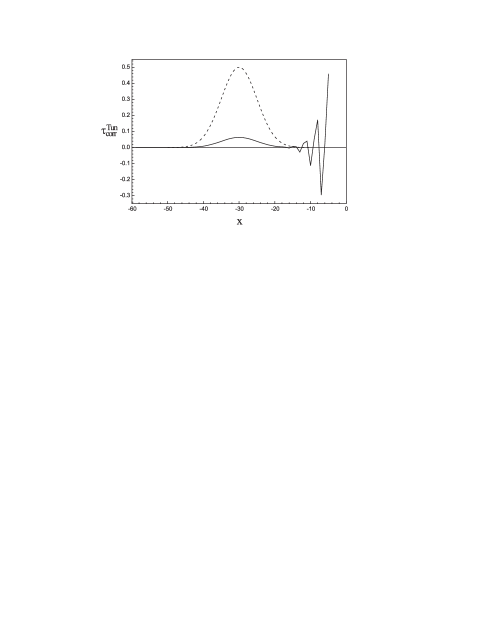
FIG. 7.: The quantity $\tau_{\text{corr}}^{\text{Tun}}\left(x\right)$ for $\delta$ function barrier with the parameters and initial conditions as in Fig. 2. The initial packet is shown with dashed line.

FIG. 8.: “Tunneling time density” for the same conditions and parameters as in Fig. 7.

$I_{1}\left(x,t\right)$ is equal to the wave function in the point $x$ at the time moment $t$ when the propagation is in the free space and the initial wave function in the energy representation is $\left|t\left(E\right)\right|^{2}\left\langle E,+\right|\Psi\rangle$. When $t\geq 0$ and $x\rightarrow-\infty$, then $I_{1}\left(x,t\right)\rightarrow 0$. That is why the initial wave packet contains only the waves moving in the positive direction. Therefore $\left\langle\hat{N}\left(X\right)\hat{T}\left(x\right)\right\rangle\rightarrow 0$ when $x\rightarrow-\infty$. From this analysis it follows that the region in which the asymptotic time is determined has to contain not only the barrier but also the initial wave packet.

In such a case from Eqs. (72) and (73) we obtain expression for the asymptotic time

$$t^{Tun}\left(x_{2},x_{1}\rightarrow-\infty\right)=\frac{1}{\left\langle\hat{N}\left(X\right)\right\rangle}\int dE\langle\Psi\left|E,+\right\rangle t^{*}\left(E\right)\left(\frac{M}{p_{E}}x_{2}-i\hbar\frac{\partial}{\partial E}\right)t\left(E\right)\left\langle E,+\right|\Psi\rangle.$$ (87)

From Eq. (76) it follows that

$$t^{Tun}\left(x_{2},x_{1}\rightarrow-\infty\right)=\frac{1}{\left\langle\hat{N}\left(X\right)\right\rangle}\left\langle\hat{T}\left(x_{2}\right)\right\rangle$$ (88)

where $\hat{T}\left(x_{2}\right)$ is defined as the probability flux integral (71). Eqs. (87) and (88) give the same value for tunneling time as an approach in Refs.[31, 32]

The integral of quantity $\tau_{\text{corr}}^{\text{Tun}}\left(x\right)$ over a large region is zero. We have seen that it is not enough to choose the region around the barrier—this region has to include also the initial wave packet location. We illustrate this fact by numerical calculations.

The quantity $\tau_{\text{corr}}^{\text{Tun}}\left(x\right)$ for $\delta$-function barrier is represented in Fig. 7. We see that $\tau_{\text{corr}}^{\text{Tun}}\left(x\right)$ is not equal to zero not only in the region around the barrier but also it is not zero in the location of the initial wave packet. For comparison, the quantity $\tau^{\text{Tun}}\left(x\right)$ for the same conditions is represented in Fig. 8.

IX Conclusion

We have shown that it is impossible to determine the time a tunneling particle spends under the barrier, because the knowledge about the location of the particle is incompatible with the knowledge whether the particle will tunnel or not. This is because the corresponding operators, given by Eqs. (2) and (10) do not commute. However, it is possible to speak about the asymptotic time, i.e., the time the particle spends in a large region.

In order to illustrate those facts, to obtain an expression of the asymptotic time and to investigate its behavior, we consider a procedure of time measurement, proposed by A. M. Steinberg [27]. This procedure shows clearly the consequences of non-commutativity of the operators and the possibility of determination of the asymptotic time. Our model also reveals the Hartmann and Fletcher effect, i.e., for opaque barriers the effective velocity is very large, because the contribution of the barrier region to the time is almost zero. We cannot determine whether this velocity can be larger than $c$, because for this purpose one has to use a relativistic equation (e.g., the Dirac’s equation).

Due to non-commutativity of operators (2) and (10) the outcome of measurements depends on particular detector even in an ideal case. This makes the measurement of the tunneling time difficult for opaque barriers, because the tunneling time is very short and the term depending on the detector increases linearly with the barrier width. This term vanishes when the time spent in a large region, including initial packet location, is measured.

REFERENCES

[1] L. A. MacColl, Phys. Rev.40, 621 (1932).
[2] E. H. Hauge and J. A. Støvneng, Rev. Mod. Phys.
61, 917 (1989).
[3] V. S. Olkhovsky, and E. Recami, Phys. Rep.
214, 339 (1992).
[4] R. Landauer and Th. Martin, Rev. Mod. Phys.
66, 217 (1994).
[5] R. Y. Chiao and A. M. Steinberg, Tunneling Times and
Superluminality, in E. Wolf, Progress in Optics XXXVII (Elsevier Science
B. V., Amstedram, 1997), p. 345.
[6] P. Guéret, E. Marclay, H Meier, Appl. Phys. Lett.
53, 1617 (1988).
[7] P. Guéret, E. Marclay, H Meier, Solid State Commun.
68, 977 (1988).
[8] D. Esteve, J. M. Martinis, C. Urbina, E. Turlot,
M. H. Devoret, P. Grabert, S. Linkwitz, Phys. Scr. Vol. T 29, 121 (1989).
[9] A. Enders, G. Nimtz, J. Phys. (France) I 3, 1089
(1993).
[10] A. Ranfagni, P. Fabeni, G. P. Pazzi, D. Mugnai, Phys. Rev. E
48, 1453 (1993).
[11] Ch. Spielmann, R. Szipöcs, A. Stingl, F. Krausz,
Phys. Rev. Lett. 73, 2308 (1994).
[12] W. Heitmann, G. Nimtz, Phys. Lett. A 196, 154 (1994).
[13] Ph. Balcou, L. Dutriaux, Phys. Rev. Lett. 78, 851
(1997).
[14] J. C. Garrison, M. W. Mitchell, R. Y. Chiao, E. L. Bolda,
Phys. Lett. A. 254, 19 (1998).
[15] M. Büttiker and R. Landauer, Phys. Rev. Lett.
49, 1739 (1982).
[16] D. Sokolovski and L. M. Baskin, Phys. Rev. A
36, 4604 (1987).
[17] C. R. Leavens, Solid State Commun. 74, 923 (1990).
[18] C. R. Leavens, Solid State Commun. 76, 253 (1990).
[19] C. R. Leavens and G.C Aers, Bohm trajectories and the
tunneling time problem, in Scanning tunneling microscopy III, edited by
R. Weisendanger and H.-J. Güntherodt (Springer, Berlin, 1993) p. 105.
[20] C. R. Leavens, Phys. Lett. A 178, 27 (1993).
[21] J. G. Muga, S. Brouard, and R. Sala, Phys. Lett. A 167, 24
(1992).
[22] A. I. Baz’ ,Sov. J. Nucl. Phys. 4, 182 (1967).
[23] R. S. Dumont, T. L. Marchioro II, Phys. Rev. A
47, 85 (1993).
[24] D. Sokolovski, J. N. L. Connor, Phys. Rev. A
47, 4677 (1993).
[25] N. Yamada, Phys. Rev. Lett. 83, 3350 (1999).
[26] S. Brouard, R. Sala, J. G. Muga, Europhys. Lett. 22,
159 (1993).
[27] A. M. Steinberg, Phys. Rev. A 52, 32 (1995).
[28] G. Iannaccone, Weak measurement and the traversal time
problem in Proceedings of Adriatico Research Conference Tunneling and Its
Implications, ed. by D. Mugnai, A. Ranfagni, and L. S. Schulman (World
Scientific, Singapore, 1997), pp. 292–309.
[29] T. E. Hartmann, J. Appl. Phys. 33, 3427
(1962).
[30] J. R. Fletcher, J. Phys. C 18, L55 (1985).
[31] V. Delgado, J. G. Muga, Phys. Rev. A 56, 3425
(1997).
[32] N. Grot, C. Rovelli, R. S. Tate, Phys. Rev. A
54, 4676 (1996).