Law of Malus and Photon-Photon Correlations:
A Quasi-Deterministic Analyzer Model

Abstract

For polarization experiments involving photon counting we introduce a quasi-deterministic eigenstate transition model of the analyzer process. Distributions accumulated one photon at a time, provide a deterministic explanation for the law of Malus. We combine this analyzer model with causal polarization coupling to calculate photon-photon correlations, one photon pair at a time. The calculated correlations exceed the Bell limits and show excellent agreement with the measured correlations of [ A. Aspect, P. Grangier and G. Rogers, Phys. Rev. Lett. 49 91 (1982)]. We discuss why this model exceeds the Bell type limits.

I INTRODUCTION

Macroscopic electromagnetic field theory leads directly to the law of Malus for light polarization measurements. For experiments where the distributions are accumulated from in-sequence photon counting, does the law of Malus still hold, and if so, what gives rise to it? Measurements using a thin polarizing film have supported the Malus formula for in sequence photon counting [1]. In these experiments where photons are counted individually in detectors, it is difficult to justify the Malus distribution from macroscopic field arguments. Past efforts to explain the law of Malus for in-sequence photon counting experiments, as well as photon-photon correlations, with hidden variable models have been unsuccessful [2, 3, 4]. These models involve a strong probability component.

Could we successfully explain the law of Malus and measured correlations by replacing the probability feature by a deterministic decision process, accumulating the distributions one particle, or particle pair at a time? The affirmative answer to this question is the focus of this paper. A deterministic trajectory model [5] has been previously used to explain ”ghost diffraction” patterns [6]. Here, we introduce a quasi-deterministic model of the analyser process. This model involves an independent stochastic variable in each analyzer, and a deterministic criterion for selecting the polarization eigenchannel in the analyzer. In this model, photons are viewed as field wave packets and trajectory calculations are not involved.

We use this model in detailed calculations to explain the law of Malus for in-sequence photon counting. We then use this same model to successfully explain some well known photon-photon correlations measurements of [7, 8, 9]. In [10] we use this quasi-deterministic analyzer model to sucessfully explain the proton-proton correlations of [11], as well as the four-angle photon-photon correlations of Aspect et al. [8]. This model makes use of causal polarization coupling between photons in a pair and local stochastic variables.

II STOKES REPRESENTATION OF THE EIGENVALUE PROBLEM

For crystal beam splitters, beam separation is based on eiegenstates, and in particular, the eigenvalues of the refractive index matrix [12]. Because of the difference in the eigenvalues for the e and o eigenstates, it is possible to separate these states. Because of the dependence on the eigenvalues, we call this type of splitter an eigenvalue splitter. The quasi-deterministic model described in detail below is based on eigenchannel selection. Stern-Gerlach type analyzers for spinors are likewise eigenvalue splitters. In the model described here, we introduce a particular stochastic variable in the refractive index matrix. Changing this particular variable does not affect the eigenvalues, so that the usual beam separation arguments are unaffected.

Polarization is conveniently represented by Stokes variables and rotations on the Poincare’ sphere. Stokes representations for both spinors and vectors are similar and well developed [13]. To formulate this eigenstate transition model, we first rewrite certain relations contained in the generic two-component eigenvalue equation in terms of a convenient Stokes variable representation. All analysis here involves a two dimensional complex representation for the field.

Consider a Hermitian matrix with elements $h_{11}=a$, $h_{22}=d$, $h_{12}=h\exp(-\imath\phi)$, and $h_{21}=h\exp(\imath\phi)$, where $a$, $d$, $h$, and $\phi$ are real. With $\Psi^{T}={\left[\Psi_{x},\Psi_{y}\right]}$, $\Psi_{x}=A\cos(\beta)\exp(\imath\alpha_{x})$ and $\Psi_{y}=A\sin(\beta)\exp(\imath(\alpha_{x}+\delta)$, we write the matrix eigenvalue equation $h\Psi=\lambda\Psi$ in component form as follows.

$$(a-\lambda)\cos(\beta)+h\exp(\imath(\delta-\phi))\sin(\beta)=0$$ (1)

$$h\exp(-\imath(\delta-\phi))cos(\beta)+(d-\lambda)\sin(\beta)=0$$ (2)

In terms of the above variables, the two eigenvalues are given by the following formula.

$$\lambda_{\pm}=(a+d\pm\sqrt{(a-d)^{2}+4h^{2}})/2$$ (3)

We employ two Stokes sets $S$ and $P$ that represent the field and matrix respectively. In terms of the field variables above, the components of $S$ have the familiar [13] form $S_{0}=\Psi^{\dagger}\Psi$, $S_{1}=S_{0}\cos(2\beta)$, $S_{2}=S_{0}\sin(2\beta)\cos(\delta)$, and $S_{3}=S_{0}\sin(2\beta)\sin(\delta)$. The components of $P$ are given by $P_{0}=\sqrt{(a-d)^{2}+4h^{2}}$, $P_{1}=P_{0}\cos(2\alpha)$, $P_{2}=P_{0}\sin(2\alpha)\cos(\phi)$ and $P_{3}=P_{0}\sin(2\alpha)\sin(\phi)$, where $\tan(2\alpha)=2h/(a-d)$. In terms of these components of $S$ and $P$, we can extract from equations (1), (2), and (3) the following relations.

$$\textbf{{P}}\cdot\textbf{{S}}=\pm P_{0}S_{0}$$ (4)

$$S_{3}P_{2}-S_{2}P_{3}=0$$ (5)

$$S_{1}P_{1}=\pm(P_{1})^{2}S_{0}/P_{0}$$ (6)

Equation (5) means $\sin(\delta-\phi)=0$ and follows directly from the imaginary component of (1) and (2).

The vectors S and P represent points on two Poincare’ polarization spheres with common centers but with different radii. The radius of the $S$ sphere is given by $S_{0}=\Psi^{\dagger}\Psi=A^{2}$. The radius of the $P$ sphere is given by $P_{0}=\lambda_{+}-\lambda_{-}$. The Stokes variables rotate with twice the rotation angle of the field components. If the space coordinates are rotated by $\theta$ say, the Stokes variables for a spinor field are rotated by $\theta$ also, whereas the Stokes variables for a vector field are rotated by $2\theta$.

In this model, an incident field makes a transition to an eigenstate described by equations (4), (5), and (6). From (6) we see that the eigenvalue sign choice in (3) is related to the sign of the product $S_{1}P_{1}$. We will make use of this relation in the deterministic transition criteria discussed below.

III STOCHASTIC ANALYZER VARIABLE

The traditional e and o rays of classical macroscopic electro-optics correspond to two points on opposite sides of the Poincare’ sphere indicated by $S_{1}=\pm S_{0}$ where in the diagonal frame we have $P_{1}=P_{0}$ for one crystal type. The two eigenvalues, on which the separation decision is made, determine the $P$ sphere radius via $\lambda_{+}-\lambda_{-}=P_{0}$, but not the direction of P. For a fixed relative phase $\phi$, this gives one free variable for the matrix Stokes vector.

The point of view here is that the classical matrix Stokes vector used for a macroscopic field of many photons does not necessarily represent the matrix Stokes vector experienced by individual photons. The first assumption of this model (The distributive assumption) is that the P vectors experienced by individual incident pulses are distributed in the one free variable, at least for the surface transition region. For a given incident pulse, we randomly select this degree of freedom of P from a distribution described below.

There are two questions related to the depth $(z)$ dependence in this model. First, are the residual deviations of $P_{1}(z)$ from the macroscopic field value only surface effects, rapidly decreasing with depth into the crystal, or, do they extend throughout the crystal? Both cases give the same correlations, and both cases give rise to the law of Malus. To correctly describe the correlations, or the law of Malus, it is only necessary with the transition criterion described below, that the surface value $P_{1}(0)$ is selected from a distribution described below. For a macroscopic field of many photons, one would not expect to have a distributive P vector because of averaging. It is therefore doubtful that we can obtain information about this distribution question with experiments using a macroscopic field of many photons.

Second, at what depth into the crystal does the incident field change so that equations (4), (5), and (6) are satisfied? This transition-depth problem in general has been the subject of debated over many years [14]. Unfortunately, the analysis here provides no answer to these questions. The presence of a local stochastic variable should have some observable affect. Indeed, it does. Within this model, this stochastic variable makes it possible to correctly describe features of both the law of Malus and photon-photon correlations. With the distribution selected, the average of $P_{1}(0)$ is the classical macroscopic matrix stokes variable.

IV STOCHASTIC VARIABLE SAMPLING

For a frame attached to the crystal analyzer (say aligned with the e and o rays), we can partition the matrix Poincare’ sphere with hemispheres indicated by the sign of $P_{1}$. However, viewed from a frame attached to one analyzer, this partition for the other analyzer is rotated. With respect to an analyzers attached frame, we choose P by choosing $2\alpha$ via $2\alpha=arg$ where $arg=\arccos(u)-\pi/2$ and $u$ is selected uniformly from the interval $[-1,1]$. For our linear polarizer, we have $\cos(\phi)=\pm 1$ in the crystal frame. Viewed from a frame fixed to the first analyzer, the $\textbf{{P}}^{\prime}$ hemisphere axis for the second analyzer is rotated from the first by $q=\theta$ for spinors and $q=2\theta$ for vectors. In this fixed reference frame, sampling for the second analyzer is made using $2\alpha^{\prime}=arg(u^{\prime})\pm q$ where $u^{\prime}$ is selected uniformly from the interval $[-1,1]$, but independent of $u$. The independence of the selection of $u$ and $u^{\prime}$ represents a local stochastic element of this theory, and is the reason why we call this a quasi-deterministic model.

One should ask if the above sampling distribution is the only distribution that can successfully described the data. There are many distributions with which one can exceed the Bell limits in this model. The above distribution and a Gaussian distribution with approximately the same width are the only two distributions that the author has found to date that correctly describe the data for both the law of Malus and the photon-photon correlations.

V DETERMINISTIC TRANSITION CRITERION

The second assumption of this model (The deterministic assumption) is that the incident pulse makes a transition to one eigen-channel or the other, and that the choice is made with a deterministic criteria based on initial conditions of the incident pulse at the analyzer and the randomly selected P. From (5) we see that the sign of $S_{1}P_{1}$ indicates the eigen-channel choice. We indicate this product as a function of the depth $(z)$ into the crystal, as follows.

$$T(z)=S_{1}(z)P_{1}(z)$$ (7)

The deterministic criteria on which the calculations here are based is that the sign of $T(z)$ after the transition is the same as, and determined by the sign of $T(0)$. For a given value for $S_{1}(0)$ and $P_{1}(0)$ we make the eigen-channel decision by testing the sign of $T(0)$. In these calculations, we only use one of the three equations (4), (5), and (6). Modeling transition criteria using all three equation is a subject of ongoing study by the author.

VI LAW OF MALUS

In the study here, we use two deterministic analyzers in sequence, with the second rotated at an angle $\theta$ relative to the first. We view the second analyzer in the reference frame of the first. The calculations are made one photon at a time. We use the same incident number of photons at each relative angle. The notation $(+,-)$ indicates the configuration for photons that exit the $(+)$ channel of the first analyzers and the $(-)$ channel of the second. To illustrate the statistical nature of the distributions, we make calculations for both a small ($100$), and a large ($40000$) number of incident photons. For the small number case, the accumulated photon counts at each angle for the $(+,+)$ configuration are indicated by the solid circles in Fig. 1. The fluctuations represent the approximate Poisson statistics of the sampling. The output for the large number case for the $(+,+)$ configuration is indicated by the solid circles in Fig. 2. The solid line represents the scaled Malus formula $N\cos^{2}(\theta)$ where $N$ is half the incident photons. The solid squares in Fig. 2 represent the accumulated distribution for the $(-,+)$ case. The dashed line represents the formula $N\sin^{2}(\theta)$. From these results, it is clear that this quasi-deterministic hidden variable model clearly gives rise to the law of Malus for in-sequence photon counting.

VII PHOTON-PHOTON CORRELATIONS

To make calculations for photon-photon coincidence measurements, we use two deterministic analyzer models to represent the two receiving analyzers. Pair counts are accumulated via deterministic calculations, one photon pair at a time. The parameters $u$ and $u^{\prime}$ for the two analyzers are sampled as indicated above, but independently of each other. Pair counts for the four different coincidence combinations are represented here by $N_{++}$ ,$N_{+-}$ , $N_{-+}$ and $N_{--}$ . For instance $N_{+-}$ is the count for the number of pairs with a $(+)$ for the first analyzer an $(-)$ for the second analyzer. The correlations are calculated using the function $\gamma(\theta)=(N_{++}+N_{--}-N_{+-}-N_{-+})/N$ [15], where $N=N_{++}+N_{--}+N_{+-}+N_{-+}$ is the total number of pairs counted. For the causal coupling, we used $S_{1}^{\prime}(0)=S_{1}(0)$ where the parameter $2\beta$ was chosen randomly from the interval $[0,2\pi]$. In the correlation calculations here, the deciding information is in the common sign of the first factors in the transition functions (7) for each analyzer. It is only necessary that $S_{1}(0)$ and $S_{1}^{\prime}(0)$ have the same sign. In Fig. 3 the solid circles represents $2N_{++}/N$. This curve follows the $\cos^{2}(\theta)$ formula, and agrees well with the coincidence measurements of [7, 8], as well as the results reported in [9] for the coincidence data obtained using a narrow spectral bandwidth and a thin crystal for the down-conversion process.

The solid circles in Fig. 4 represent the calculated correlation function [15, 8]. The four pair-counts were accumulated, one photon pair at a time. Calculations are made using about $10000$ photon pairs at each angle. The solid line in Fig. 4 represents the formula of quantum mechanics. The two curves show excellent agreement with each other and with the measurements of [8]. We emphasize that all contributions to $\gamma(\theta)$ were calculated using the four pair counts only so there is no chance that an accidental scale factor can be included.

VIII EXCEEDING BELL’S LIMITS

The causal polarization link between the two photons in a pair produces an angular correlation link even with the presence of the local stochastic variables in the analyzers. This angular dependent link is why the usual inequality Bell’s theorem [16, 17] doesn’t apply to this quasi-deterministic analyzer model.

To explain this angular dependence in more detail, consider the transition function $T(0)=S_{1}(0)P_{1}(0)=S_{0}P_{0}\cos(2\beta)\cos(arg(u))$ for the first analyzer and $T^{\prime}(0)=S_{1}(0)P_{1}^{\prime}(0)=S_{0}P_{0}\cos(2\beta)\cos(arg(u^{\prime})+2\theta)$ for the second. Both expressions have the same first factor which arises because of the causal coupling between the photons. If we don’t use this causal coupling, (e.g. choose the angles in the first two factors completely independent of each other), the correlations vanish. The independent parameters $u$ and $u^{\prime}$ represents local stochastic variables of this theory. Within the distribution range, and depending on the angle $2\theta$, there are certain values of $u^{\prime}$ for which the second factor in $T^{\prime}(0)$ can be negative, and certain values for which this factor is positive. Because of these stochastic variables, we cannot know which pair count combination (such as $(+-)$) we have until after the coincident count is made. However, we still have distribution information. The number of times the second factor in $T^{\prime}(0)$ is positive depends on the angle $2\theta$. As a consequence, we have correlations in the distributions which depend on the relative angle. The presence of the local stochastic variables, a necessary part of this theory, does not destroy all causal correlation information. We emphasize that this is a causal non-local effect, and should not be confused with instantaneous action at a distance effects. The correlations do not depend on the distance between the analyzers, as long as the causal polarization link between the photons remains intact until the photons reach the analyzers.

In comparison with the results here, it is worth commenting on ”Bell’s theorem without inequalities” type arguments that have appeared [2, 18]. In studies leading to this work, the author has calculated correlations with many different hidden variable probability models, and not found one, no matter what sampling distribution used, that agrees with the deterministic model and quantum mechanics. This finding seems to be consistent with the studies of hidden variable probability models by previous authors [2, 18]. Replacing the deterministic transition criterion at the analyzers with probability amounts to throwing away much of the detailed correlations information.

IX CONCLUSIONS

We have introduced a quasi-deterministic analyzer model, and have demonstrated with detailed calculations, that the law of Malus and photon-photon correlations can be explained with a causal hidden variable theory, via accumulation, one photon or photon pair at a time. If we omit the causal coupling, the correlations are lost. If we don’t use a stochastic variable in the analyzer we can’t explain the data for the law of Malus nor the correlations. If we replace the local deterministic decision process in the analyzers with one based on probability, the correlations are reduced. In simple terms, if we throw away the information, we can’t explain the data. Calculations to successfully explain some other quantum measurements have been completed and will be reported on elsewhere [10].

In this paper, we have only considered polarization correlations. The essential features of this model are a causal link variable, local analyzer variables, and a deterministic decision criterion. Studies using a model with these features to describe energy-time photon correlations [19, 20, 21] are underway.

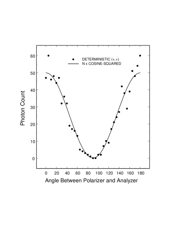
FIG. 1.: Malus distribution for few photons. Calculated using the deterministic
analyzer model: Solid circles indicate the photon accumulation. Counts are
accumulated one photon at a time.

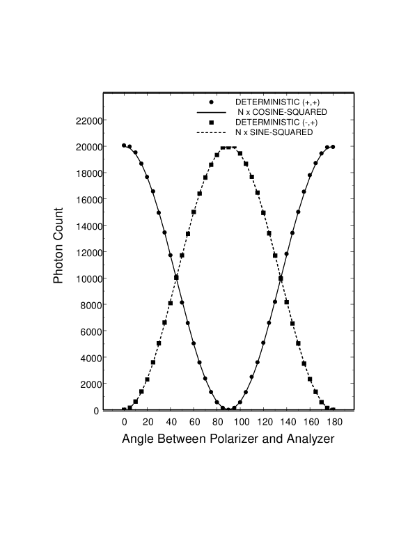
FIG. 2.: Malus distribution for many photons. Calculated using the deterministic
analyzer model: Solid circles indicate the photon accumulation. Counts are
accumulated one photon at a time.

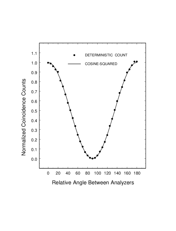
FIG. 3.: Normalized photon-photon coincidence counts $2N_{++}/N$ versus relative
angle: These calculations used the quasi-deterministic analyzer model. The
distributions are accumulated one photon pair at a time.

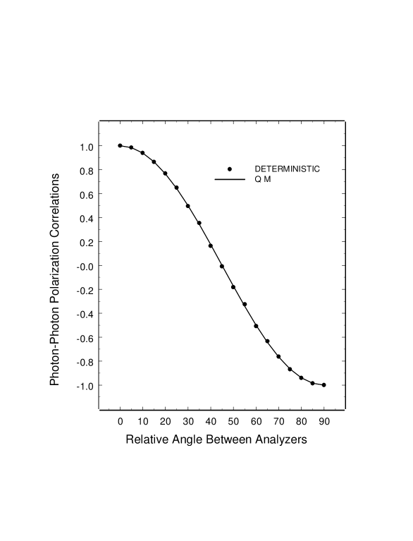
FIG. 4.: Photon-photon correlations calculated using the quasi-deterministic analyzer
model: Solid circles represent the calculated correlation obtained via accumulation,
one photon pair at a time. The line indicates the quantum mechanics prediction.

REFERENCES

- [1] Papaliolios C. (1967). Phys. Rev. Lett. 18, 622.
- [2] Belinfante F. J. (1973). A Survey of Hidden Variable Theories, (Pergamon Press, New York). See Ch. 5 for discussion of earlier studies on the law of Malus with hidden variable theories.
- [3] Ballentine L. E. (1987). Am. J. Phys. 55 (9) 785. This is a resource article on this topic.
- [4] Afriat A. and Selleri F. (1999). The Einstein Podolski and Rosen Paradox, (Plenum Press, New York). This recent book includes many references to earlier studies.
- [5] Dalton B. J. (1997) in Causality and Locality in Modern Physics, Eds. G. Hunter, S. Jeffers, and J-P. Vigier, (Kluwer-Academic Publishers, Dordrecht, The Netherlands).
- [6] Strekalov D.V., Sergienko A. V., Klyshko D. N., and Shih Y. H., (1993). Phys. Rev. Lett, 74 (18) 3600.
- [7] Aspect A., Grangier P. and Rogers G. (1981). Phys. Rev. Lett. 47, 460.
- [8] Aspect A., Grangier P. and Rogers G., (1982). Phys. Rev. Lett. 49, 91.
- [9] Alley C. O., Keiss T. E., Sergienko A. V. and Shih Y. H. (1994). in Frontiers of Fundamental Physics, eds. M. Barren and F. Seller ( Plenum Press, New York).
- [10] Dalton Bill. Two particle correlations via quasi-deterministic analyzer model. Submitted for publication.
- [11] Lamehi-Rachti M. and Mittig W. (1976). Phys. rev. D 14 (10), 2543 .
- [12] Yariv A. and Yeh P., (1984). Optical Waves in Crystals, (Wiley Interscience, New York).
- [13] McMaster W. H., (1954). Am. J. Phys. 22 (6) 351.
- [14] Fearn H., James D. F. V. and Milonni P. W. (1996). Am. J. Phys. 64, (18), 986.
- [15] Garuccio A. and Rapisarda V. (1981). Nuovo Cimento, 65A, 269.
- [16] Bell, J. S. (1964) Physics 1, 195.
- [17] Clauser J. F., Horne M. A., Shimony A., and Holt R. A., (1969) Phys. Rev. Lett. 23, 880.
- [18] Greenberg D. M., Horne M. A., Shimony A. and Zeilinger A. (1990). Am. J. Phys. 58, (12) 1131.
- [19] Franzon, J. D. (1989) Phys. Rev. Lett. 62, 2205.
- [20] Tittle W., Brendel J., Zbinden H., and Gisin N., (1998) Phys. Rev. Lett 81, 3563.
- [21] Tittle W., Brendel J., Zbinden H., and Gisin N., (2001) Preprint from ArXiv:quant-ph/9806043.