Abstract

We provide a rate distortion interpretation of the problem of quantum data compression of ensembles of mixed states with commuting density operators. There are two versions of this problem. In the visible case the sequence of states is available to the encoder and in the blind or hidden case the encoder may access only a sequence of measurements. We find the exact optimal compression rates for both the visible and hidden cases. Our analysis includes the scenario in which asymptotic reconstruction is imperfect.

1 Introduction

Claude Shannon created the foundations of information theory, a mathematical theory of communication, in his landmark 1948 paper [1]. However, until fairly recently few attempts were made to study the transmission and processing of quantum states. The excellent survey paper [2] provides considerable motivation for the study of quantum information theory. Important application areas include quantum cryptographic protocols that are more secure than and quantum computers that are dramatically faster than their classical counterparts.

The first problem that Shannon addressed in [1] was the ultimate data compression achievable on the output of a discrete information source. Shannon initially considered the set of encoding rules for which the source sequence can be perfectly retrieved from the encoded sequence, at least with high probability. For any discrete, stationary, and ergodic source, Shannon defined the entropy of the source as a function of the probabilities of the source and demonstrated that the minimum achievable average number of code symbols per source symbol is the entropy of the source. Later in another paper [3], Shannon also treated the problem of encoding a source given a fidelity criterion or a measure of the distortion for a representation of the source output. The goal in this case is to minimize the expected distortion attainable at a particular rate. For a wide class of distortion measures and source models, Shannon provided a generalization of the source entropy, known as the rate distortion function, which establishes the exact trade off between the distortion level and the compression rate.

An important problem in the field of quantum information theory is the generalization of classical results on data compression to the quantum domain. To our knowledge, the literature thus far treats quantum analogs of discrete, memoryless sources and assumes that the reconstruction must have arbitrarily high fidelity in the limit as the source string length approaches infinity.

In order to describe a discrete, memoryless quantum source, we must first define pure and mixed quantum states. The state space of a quantum system is a complete description of the properties of the particles in the system. It includes information about positions, momentums, polarizations, spins, and so on. The state space is commonly modelled by a Hilbert space of wave functions. The mathematical tools used for the study of quantum information systems are finite dimensional complex vector spaces with an inner product that are spanned by abstract wave functions. A thorough discussion of mathematical conventions and terminology which are standard in quantum mechanics can be found in [4]. In particular, a state is a ray in a Hilbert space, where a ray is defined as an equivalence class of unit norm vectors that differ by multiplication by a nonzero complex scalar. If we are looking at a subsystem of a larger quantum system, then the state of the subsystem is not necessarily a ray. If the state of the subsystem is a ray, then the state is called pure and otherwise it is called mixed. When we are considering these subsystems, the state of the system is represented by a density operator, i.e., a positive semi-definite matrix with unit trace. In the special case of a pure state, the density operator is the rank one outer product of the corresponding ray with its conjugate transpose. For a mixed state, the density operator is a convex combination of the density operators of two or more pure states.

A discrete, memoryless quantum information source is an ensemble of density operators $\rho_{1},\,\dots,\,\rho_{M}$ emitted with probabilities $\alpha_{1},\,\dots,\,\alpha_{M}$. Each density operator corresponds to a pure or a mixed state. The goal of the quantum data compression problem formulated in [5] is to compress a sequence of pure quantum states into the smallest possible Hilbert space with arbitrarily good reconstruction fidelity in the limit as the sequence length approaches infinity. In the special case where the ensemble consists of only pure states, the problem has been solved in [5], [6], [7]. The more general problem where the ensemble contains at least one mixed state was first mentioned in [8]. In this case, the optimal compression rate is unknown [9], [10], [11], but these papers provide upper and lower bounds on the best achievable compression rates.

When the matrices corresponding to the density operators for an ensemble of mixed and/or pure states commute, the quantum compression problem has been reformulated in [11] as an equivalent classical information theory problem in which probability distributions are compressed and communicated. Our analysis will be in terms of this formulation. The problem of optimal mixed state coding has been considered in two different scenarios. In the first case, called the visible source case, the encoder knows the precise sequence of states or probability distributions that it is transmitting. In the second case, called the hidden source case, the encoder only has access to a measurement or “side information” sequence. Each entry of this second sequence is found by taking a measurement of the corresponding state; i.e., taking one experimental outcome of the probability distribution of the analogous entry in the original sequence. Elsewhere in the quantum information literature this is called the blind case, but the terminology “hidden” is more standard in the communications literature. References [9], [10], and [11] provide lower and upper bounds for the optimal rate of asymptotically faithful compression which apply to both variants of the problem.

We provide a rate distortion interpretation of the problem which unifies the analysis of both variants and leads to the exact optimal rates for both the visible and blind versions. Furthermore, the rate distortion framework leads to a natural generalization of the quantum compression problem in which the expected fidelity of reconstruction is asymptotically bounded from below but is not necessarily perfect. To our knowledge, this problem has not been addressed earlier in the literature. Our techniques provide the optimal compression rate for the both the visible and blind commuting cases in this setting.

It has come to our attention that [12] presents an alternate proof of the achievability of the lower bound in the visible, commuting case where reconstruction is asymptotically perfect.

1.1 Transmitting Probability Distributions

Suppose that we have an ensemble of $M$ states with the corresponding discrete probability mass functions $P_{1},P_{2},\dots,P_{M}$ that assume outcome values from the alphabet ${\cal Y}=\{1,\dots,N\}$. We represent the alphabet $\{1,\dots,M\}$ by ${\cal X}$. Let $p_{i,j},\;i\in{\cal X},\;j\in{\cal Y}$ denote the probability that a measurement of the $i^{\mbox{th}}$ state leads to outcome value $j$. Hence, $p_{i,j}\;\geq\;0,\;i\in{\cal X},\;j\in{\cal Y},$ and $\sum_{j=1}^{N}p_{i,j}\;=\;1,\;i\in{\cal X}.$

Assume there is a memoryless source emitting a sequence of the mass functions. In other words, there is a probability distribution on ${\cal X}$ and with probability $\alpha_{i}$ the source emits state $i$. The source simultaneously produces a second sequence on ${\cal Y}$ which can be viewed as side information. When the source emits state $i$, it also emits a side-information output symbol $j\in{\cal Y}$ with probability $p_{i,j}$. Let $\{X_{\ell}\}_{\ell\geq 1}$ and $\{Z_{\ell}\}_{\ell\geq 1}$ be the output of the source corresponding to the sequence of states and the sequence of side information, respectively. For the original problem posed in [11], we wish to consider codes in which a receiver that knows the source model generates a sequence $\{Y_{\ell}\}_{\ell\geq 1}$ of output values that fall in the “strongly typical set” (see, e.g., [13, §13.6]) for the state sequence $\{X_{\ell}\}_{\ell\geq 1}$. More specifically, for each state $i$ the relative frequencies of the $N$ output symbols corresponding to the positions where $i$ is the state emitted from the source should asymptotically converge to the probability mass function $P_{i}$ with probability $1$. In other words, we measure the fidelity of the output sequence $\{Y_{\ell}\}_{\ell\geq 1}$ through the empirical distribution of sequences of pairs $\{(X_{\ell},Y_{\ell})\}_{\ell\geq 1}$. In practice, coding is performed from finite strings $X^{L}=X_{1},X_{2},\dots,X_{L}$ to output strings $Y^{L}=Y_{1},Y_{2},\dots,Y_{L}$. Pick a block length $L$ and let $P^{e}_{X^{L}Y^{L}}(i,j)$ denote the sample frequency of state and output pairs $(X_{l},Y_{l})=(i,j)$ over the range $l\in\{1,\dots,L\}$. Then for the compression problem with asymptotically perfect reconstruction we require the Bhattacharyya-Wootters overlap [11, p. 9] of the true probabilities $\alpha_{i}\,p_{i,j}$ and the empirical frequencies of the state and output pairs to be arbitrarily close to 1 in the limit as $L$ approaches infinity. More precisely, we choose our code to satisfy the constraint

$$\mbox{Pr}\left(\left(\sum_{i=1}^{M}\sum_{j=1}^{N}\sqrt{\alpha_{i}\,p_{i,j}\,P^{e}_{X^{L}Y^{L}}(i,j)}\right)^{2}<1-\varepsilon\right)\;<\;\delta$$ (1)

for arbitrarily small positive constants $\delta$ and $\varepsilon$ whenever $L$ is sufficiently large. The code may use probabilistic processes for the encoding and/or decoding. The objective of the encoder is to compress the state sequence as much as possible.

The source model for this problem superficially resembles the composite source models discussed in [14, §6.1]. The key difference is the reversal of what is viewed as the side information sequence and what is viewed as the primary source sequence. For this reason, the analysis techniques developed for that source coding problem do not appear to apply to this setting.

There are two obvious upper bounds to the minimum average number of bits per symbol required in the encoding. One of these bounds applies to both the visible and the blind versions of the compression problem and the other applies only to the visible case. For the visible problem, the encoder may simply transmit the sequence $\{X_{\ell}\}_{\ell\geq 1}$ and the decoder may use the appropriate probability mass function every time it receives a state to generate the output sequence. With this algorithm, the expected number of bits per symbol used by the encoder can come arbitrarily close to the entropy [1] of the state alphabet:

$$-\sum_{i=1}^{M}\alpha_{i}\log_{2}\alpha_{i}.$$

Another possibility for either the blind or the visible case is for the encoder to transmit the sequence $\{Z_{\ell}\}_{\ell\geq 1}$ and the decoder to use the sequence without modifying it. The entropy of this sequence is

$$-\left(\sum_{i=1}^{M}\sum_{j=1}^{N}\alpha_{i}p_{i,j}\right)\log_{2}\left(\sum_{i=1}^{M}\sum_{j=1}^{N}\alpha_{i}p_{i,j}\right).$$

It is easy to find situations where both of these procedures are suboptimal. Consider the case where the $M$ probability mass functions are identical, $\alpha_{i}=1/M$ for all states $i$, and $p_{i,j}=1/N$ for all pairs of states $i$ and output symbols $j$. In this case, transmitting the sequence $\{X_{\ell}\}_{\ell\geq 1}$ will require $\log_{2}M$ bits per symbol on average and transmitting the sequence $\{Z_{\ell}\}_{\ell\geq 1}$ will require $\log_{2}N$ bits per symbol on average. Here the optimal coding procedure for both the visible and blind versions of the problem would be to have the encoder transmit nothing and the decoder generate independent and equiprobable output symbols. This coding procedure uses the ideal of zero bits per symbol.

It is possible to modify the entropy upper bound for some sources to avoid the simple counterexample above. Suppose that there are two or more output symbols $j$ which have a “common randomness;” i.e., for which the $p_{i,j}$ are equal for all $i\in{\cal X}$. Then an encoding strategy would be to introduce an erasure symbol, to replace all occurrences of output symbols with common randomness in $\{Z_{\ell}\}_{\ell\geq 1}$ with the erasure symbol, and to encode the resulting sequence to its entropy. The decoder will not modify the ordinary symbols, and when it sees an erasure symbol it will generate a symbol of “common randomness” with the appropriate conditional probability. In the case where $p_{i,j}>0$ for all pairs $(i,j)\in{\cal X}\times{\cal Y}$, we will show that for the blind version of the problem with asymptotically perfect fidelity it is impossible to do better than this modified entropy bound. Some additional care needs to be provided in specifying the solution for the blind version of the problem when there are pairs $(i,j)\in{\cal X}\times{\cal Y}$ with $p_{i,j}=0$, but the solution is in the form of a mutual information.

[10] and [11] prove that a lower bound to the optimal compression ratio for both versions of the problem with asymptotically perfect fidelity is the mutual information between the state alphabet and the output alphabet

$$\sum_{i=1}^{M}\sum_{j=1}^{N}\alpha_{i}p_{i,j}\log_{2}p_{i,j}-\left(\sum_{i=1}^{M}\sum_{j=1}^{N}\alpha_{i}p_{i,j}\right)\log_{2}\left(\sum_{i=1}^{M}\sum_{j=1}^{N}\alpha_{i}p_{i,j}\right),$$ (2)

but leaves open the question whether this lower bound is attainable in either the visible or the blind variants. We will establish that it is achievable for the visible version of the problem.

Our analysis takes advantage of the tools of rate distortion theory. The quantum information literation thus far has focused upon the Bhattacharyya-Wootters overlap (see (1)) as a way to measure the closeness of two probability distributions. This overlap is non-negative and is equal to one exactly when the two probability distributions are identical. An equivalent and opposite way to measure the closeness of two probability distributions is to discuss their “distance” or the distortion generated by approximating one by the other. In this setting, perfect fidelity corresponds to zero distortion. The Bhattacharyya-Wootters overlap can be converted into such a distortion function by being subtracted from one. There are many other examples of interesting distortion functions that appear in the probability and classical information literature. The advantage of this interpretation is that rate distortion theory has been studied extensively since [3]. We will show that there is a very simple way to formulate and solve the problem of compressing probability distributions in the rate distortion setting. It is also straightforward to generalize these results to the case where the reconstruction fidelity is imperfect.

2 Preliminaries

We begin with several basic information-theoretic definitions. Suppose we have two discrete and finite random variables $X$ and $Y$ whose joint probability distribution is $P_{XY}$. The entropy of $X$ and conditional entropy of $X$ given $Y$ are defined as (see [13, Ch. 2])

$$H(X) =\sum_{x\in\rm{supp}(P_{X})}-P_{X}(x)\log(P_{X}(x)),$$

$$H(X|Y) =\sum_{(x,y)\in\rm{supp}(P_{XY})}-P_{XY}(x,y)\log(P_{X|Y}(x|y)),$$

where $\rm{supp}(P_{X})$ is the support of $P_{X}$, i.e., the set of $x$ such that $P_{X}(x)>0$. As done here, we will continue to write random variables with upper-case letters and values they take on with lower-case letters. The informational divergence between $P_{X}$ and $P_{Y}$ is defined as

$$D(\,P_{X}\,\|\,P_{Y}\,) =\sum_{x\in\rm{supp}(P_{X})}P_{X}(x)\,\log\left(\frac{P_{X}(x)}{P_{Y}(x)}\right),$$

and we write $D(P_{X}\|P_{Y})=\infty$ when there is an $x$ in $\rm{supp}(P_{X})$ such that $P_{Y}(x)=0$. The informational divergence is also called the “information for discrimination,” the “relative entropy” and the “Kullback-Leibler distance” [16, p. 20], [13, p. 18]. The mutual information between $X$ and $Y$ is defined as

$$I(X;Y) =D(\,P_{XY}\,\|\,P_{X}P_{Y}\,)$$

$$=H(X)-H(X|Y)$$

$$=H(Y)-H(Y|X).$$

A well-known property of these quantities is that they are all non-negative [13, Ch. 2]. Furthermore, $D(P_{X}\|P_{Y})=0$ if and only if $P_{X}(x)=P_{Y}(x)$ for all $x$ in $\rm{supp}(P_{X})$. This implies that $I(X;Y)=0$ if and only if $X$ and $Y$ are statistically independent. Two other important properties involving convexity are given as lemmas.

Lemma 2.1 ([13, p. 30]).

$D(P_{X}\|P_{Y})$ is convex in the pair $(P_{X},P_{Y})$, i.e., if $(P_{X_{\ell}},P_{Y_{\ell}})$, $\ell=1,2,\ldots,L$, are pairs of distributions, then for any nonnegative $\lambda_{\ell}$ which sum to one we have

$$\sum_{\ell=1}^{L}\lambda_{\ell}\,D\left(P_{X_{\ell}}\,\|\,P_{Y_{\ell}}\right)\geq D\left(\sum_{\ell=1}^{L}\lambda_{\ell}P_{X_{\ell}}\,\left\|\,\sum_{\ell=1}^{L}\lambda_{\ell}P_{Y_{\ell}}\right.\right).$$ (3)

Equivalently, we can view $D(P_{X}\|P_{Y})$ as a function of $P_{XY}$ and say that $D(P_{X}\|P_{Y})$ is convex in $P_{XY}$.

Let $J$ be a random variable taking on the value $\ell$ with probability $\lambda_{\ell}$, $\ell=1,\ldots,L$. We can write (3) as

$${\rm E}_{J}\left[D\left(P_{X_{J}}\,\|\,P_{Y_{J}}\right)\right]\geq D\left({\rm E}_{J}\left[P_{X_{J}}\right]\,\|\,{\rm E}_{J}\left[P_{Y_{J}}\right]\right)$$ (4)

where $E_{J}[\,\cdot\,]$ denotes expectation with respect to the random variable $J$. We will sometimes drop the subscript $J$ and write ${\rm E}[\,\cdot\,]$ if it is clear with respect to which random variable we are taking expectations.

Lemma 2.2 ([13, p. 31]).

The mutual information $I(X;Y)$ is concave in $P_{X}$ when $P_{Y|X}$ is fixed, and convex in $P_{Y|X}$ when $P_{X}$ is fixed. In other words, we have

$${\rm E}_{J}\left[I\left(X_{J}\,;\,Y_{J}\right)\right]\leq I\left({\rm E}_{J}\left[X_{J}\right]\,;\,{\rm E}_{J}\left[Y_{J}\right]\right)$$

when $P_{Y_{J}|X_{J}}$ is the same for all $J$, and

$${\rm E}_{J}\left[I\left(X_{J}\,;\,Y_{J}\right)\right]\geq I\left({\rm E}_{J}\left[X_{J}\right]\,;\,{\rm E}_{J}\left[Y_{J}\right]\right)$$ (5)

when $P_{X_{J}}$ is is the same for all $J$.

Our distortion measures will be defined in terms of the empirical probability distribution of finite-length sequences or strings. The empirical probability distribution of the length-$L$ string $x^{L}=x_{1},x_{2},\ldots,x_{L}$ with $x_{\ell}\in{\cal X}$ is defined as

$$P^{e}_{x^{L}}(a)=\frac{n_{x^{L}}(a)}{L}\quad\mbox{for all }a\in{\cal X},$$

where $n_{x^{L}}(a)$ is the number of occurrences of the letter $a$ in the string $x^{L}$ [16, p. 29],[13, p. 279]. A simple yet important property of $P^{e}_{x^{L}}$ is given by the following lemma.

Lemma 2.3.

$${\rm E}_{X^{L}}\left[P^{e}_{X^{L}}\right]=\frac{1}{L}\sum_{\ell=1}^{L}P_{X_{\ell}}.$$ (6)

Proof.

We have, for all $a\in{\cal X}$,

$${\rm E}_{X^{L}}\left[P^{e}_{X^{L}}(a)\right] ={\rm E}_{X^{L}}\left[\frac{n_{X^{L}}(a)}{L}\right]$$

$$=\frac{1}{L}{\rm E}_{X^{L}}\left[\sum_{\ell=1}^{L}1(X_{\ell}=a)\right]$$

where $1(\,\cdot\,)$ is the indicator function that is 1 if its argument is true and is 0 otherwise. Since the expectation of a sum is the sum of the expectations [17, p. 10] , we have

$$\frac{1}{L}{\rm E}_{X^{L}}\left[\sum_{\ell=1}^{L}1(X_{\ell}=a)\right] =\frac{1}{L}\sum_{\ell=1}^{L}{\rm E}_{X^{L}}\left[1(X_{\ell}=a)\right]$$

$$=\frac{1}{L}\sum_{\ell=1}^{L}P_{X_{\ell}}(a).$$

∎

2.1 Rate Distortion Theory

We describe the rate distortion problem as considered by Shannon [3] (see Fig. 1). A discrete memoryless source (DMS) produces a message string $X^{L}$ of $L$ independent and identically distributed letters from a finite alphabet ${\cal X}$. $X^{L}$ is encoded into one of $K=2^{LR}$ received strings $Y^{L}$ of $L$ letters from a finite alphabet ${\cal Y}$. The rate of the encoder is thus $R$ bits per letter, because one can represent any $y^{L}$ by a string of $LR$ bits. There is a distortion measure $d(\cdot,\cdot)$ that associates a non-negative number $d(x,y)$ with each pair $(x,y)$ of message letter $x$ and receive letter $y$. The distortion between the strings $x^{L}$ and $y^{L}$ is defined as the average of the letter-to-letter distortions:

$$d(x^{L},y^{L})=\frac{1}{L}\sum_{\ell=1}^{L}d(x_{\ell},y_{\ell}),$$

where we have abused notation by using the same symbol $d$ for the letter-to-letter and string distortions. Shannon generalized the letter-to-letter distortion measure in [3], but we will not be using that generalization here.

Figure 1: Model for the rate distortion problem.

The fundamental problem of rate distortion theory is to determine the minimum code rate $R$ such that the average distortion between $X^{L}$ and $Y^{L}$ is upper bounded by some number $\Delta$. The rate distortion function $R(\Delta)$ is thus defined as the greatest lower bound on $R$ such that ${\rm E}[d(X^{L},Y^{L})]\leq\Delta$. Shannon showed that $R(\Delta)$ has the simple form given by the following lemma.

Lemma 2.4 (Shannon [3]).

The rate distortion function of a DMS with distribution $P_{X}$ and letter-to-letter distortion measure $d(\cdot,\cdot)$ is

$$R(\Delta) =\min_{\Let@\restore@math@cr\default@tag\vbox{\halign{\hfil$\m@th\scriptstyle{#}$\hfil\cr P_{Y|X}:\\ {\rm E}[d(X,Y)]\leq\Delta\crcr}}}I(X;Y)$$

The achievability of the rate distortion function is usually demonstrated by choosing a random code as follows: the $L$ letters of each of the $2^{LR}$ code words are chosen independently using $P_{Y}$. One then associates the “typical” strings $x^{L}$, i.e., those $x^{L}$ for which $P^{e}_{x^{L}}$ is close to $P_{X}$, with one of the code words $y^{L}$ for which $P^{e}_{x^{L}y^{L}}$ is close to $P_{XY}$, where $P^{e}_{x^{L}y^{L}}$ is the empirical distribution of the $L$ pairs $(x_{\ell},y_{\ell})$. One can show that if $R>R(\Delta)$ and $L$ is large, such a code word $y^{L}$ exists and $d(x^{L},y^{L})\leq\Delta$ with high probability.

A generalization of the rate distortion problem was given by Dobrushin and Tsybakov in [15] (see Fig. 2). The new twist is that the encoder sees only a noisy version $V^{L}$ of the message $X^{L}$, where $v_{\ell}$ is generated by $x_{\ell}$ via the memoryless channel $P_{V|X}(v_{\ell}|x_{\ell})$ for all $\ell$. The DMS is sometimes called a “remote source” [14, p. 78],[16, p. 136]. We will call the DMS a hidden source, $X^{L}$ the hidden source string, $V^{L}$ the visible source string and $P_{V}$ the visible distribution. Note that if $V=X$ we have the original rate distortion problem.

Figure 2: Model for the rate distortion problem with a hidden source.

The goal is again to determine the minimum code rate $R$ such that the average distortion between $X^{L}$ and $Y^{L}$ is upper bounded by some number $\Delta$. The rate distortion function $R(\Delta)$ is thus defined as before, and Dobrushin and Tsybakov proved the following lemma.

Lemma 2.5 (Dobrushin and Tsybakov [15]).

The rate distortion function of a hidden DMS with distribution $P_{X}$, visible distribution $P_{V}$, and single-letter distortion measure $d(\cdot,\cdot)$ is

$$R(\Delta) =\min_{\Let@\restore@math@cr\default@tag\vbox{\halign{\hfil$\m@th\scriptstyle{#}$\hfil\cr P_{Y|V}:\\ {\rm E}[d(X,Y)]\leq\Delta\crcr}}}I(V;Y)$$

Note that

$$I(V;Y) =H(Y)-H(Y|V)$$

$$=H(Y)-H(Y|VX)$$

$$\geq H(Y)-H(Y|X)$$

$$=I(X;Y),$$

where the second equality follows because $Y$ is independent of $X$ given $V$, and the inequality follows because conditioning cannot increase entropy [13, p. 27]. Thus, not surprisingly, the best rate when $X^{L}$ is hidden is at least as large as when $X^{L}$ is visible.

Lemma 2.6.

The random variables of the rate distortion problem with a hidden source satisfy

$$H(Y^{L})\geq I(V^{L};Y^{L})\geq\sum_{\ell=1}^{L}I(V_{\ell};Y_{\ell})\geq L\cdot I\left(\overline{V};\overline{Y}\right),$$ (11)

where $P_{\overline{V}\,\overline{Y}}=\sum_{\ell=1}^{L}P_{V_{\ell}Y_{\ell}}/L$.

Proof.

The first inequality follows by the non-negativity of $H(Y^{L}|V^{L})$. In fact, $Y^{L}$ is usually a function of $V^{L}$ so that $H(Y^{L}|V^{L})=0$ and $H(Y^{L})=I(V^{L};Y^{L})$. The second inequality follows by

$$I(V^{L};Y^{L}) =\sum_{\ell=1}^{L}H(V_{\ell}|V^{\ell-1})-H(V_{\ell}|Y^{L}V^{\ell-1})$$

$$=\sum_{\ell=1}^{L}H(V_{\ell})-H(V_{\ell}|Y^{L}V^{\ell-1})$$

$$\geq\sum_{\ell=1}^{L}H(V_{\ell})-H(V_{\ell}|Y_{\ell}).$$

The third inequality follows by viewing the sum over the $I(V_{\ell};Y_{\ell})$ as $L$ times ${\rm E}_{J}[I(V_{J};Y_{J})]$, where $J$ takes on the value $\ell$ with probability $1/L$ for $\ell=1,\ldots,L$. The bound (5) then gives the desired result. ∎

3 Quantum Rate Distortion

We deal with the visible and hidden (or blind) source problems simultaneously by introducing an auxiliary string $Z^{L}$ to the model of Fig. 2 (see Fig. 3). $Z^{L}$ represents the outcomes of measurements and is called side information in Section 1.1. The terms of $Z^{L}$ take on values in the alphabet ${\cal Z}$ and are generated together with $V^{L}$ as outputs of a memoryless channel $P_{VZ|X}$.

Figure 3: Model for the quantum rate distortion problem.

We are interested in string distortion measures $d(\cdot,\cdot)$ that depend on $(x^{L},y^{L})$ only through the empirical distribution $P^{e}_{x^{L}y^{L}}$. Thus, with some abuse of notation we can write $d(x^{L},y^{L})=d(P^{e}_{x^{L}y^{L}})$. For example, using (1) the Bhattacharyya-Wootters distortion measure could be defined as

$$d(P^{e}_{x^{L}y^{L}}) =1-\left[\sum_{x\in{\cal X},z\in{\cal Z}}\sqrt{P_{XZ}(x,z)\,P^{e}_{x^{L}y^{L}}(x,z)}\right]^{2},$$ (12)

where $Z$ plays the role of the measurement outcomes in Section 1.1. The visible case has $V=X$ while the hidden case can have $V\neq X$ and has $V=Z$. As a second example, a natural information-theoretic distortion measure is the informational divergence

$$d(P^{e}_{x^{L}y^{L}}) =D\left(P^{e}_{x^{L}Z}\|P^{e}_{x^{L}y^{L}}\right),$$ (13)

where $P^{e}_{x^{L}Z}(a,b)$ is defined as $\left[\sum_{c\in{\cal Y}}P^{e}_{x^{L}y^{L}}(a,c)\right]P_{Z|X}(b|a)$ for all $a\in{\cal X}$ and $b\in{\cal Z}$, i.e., $P^{e}_{x^{L}Z}=P^{e}_{x^{L}}\,P_{Z|X}$. Observe that low distortion is achieved only if the empirical distribution of $(x^{L},y^{L})$ is close to the desired distribution $P^{e}_{x^{L}Z}$.

We next impose an additional restriction on $d(\cdot)$, namely that $d(P_{XY})$ be convex in $P_{XY}$, i.e.,

$${\rm E}_{J}\left[d\left(P_{X_{J}Y_{J}}\right)\right]\geq d\left({\rm E}_{J}\left[P_{X_{J}Y_{J}}\right]\right),$$ (14)

where $J$ is a finite random variable. The distortion measure (13) meets this requirement by Lemma 2.1. The distortion measure (12) also meets this requirement since, for $\lambda_{\ell}\geq 0$ and $\sum_{\ell}\lambda_{\ell}=1$, we have

$$1-\left[\sum_{x,z}\sqrt{\sum_{\ell}\lambda_{\ell}a_{\ell}(x,z)}\right]^{2} \leq 1-\sum_{\ell}\left[\sum_{x,z}\sqrt{\lambda_{\ell}a_{\ell}(x,z)}\right]^{2}$$

$$=\sum_{\ell}\lambda_{\ell}\left\{1-\left[\sum_{x,z}\sqrt{a_{\ell}(x,z)}\right]^{2}\right\},$$

where $a_{\ell}(x,z)=P_{XZ}(x,z)\,P^{e}_{X_{\ell}Y_{\ell}}(x,z)$ and where the first step follows by Minkowski’s inequality [18, p. 523].

We call the problem of finding the rate distortion function for this set-up the quantum commuting density operator (quantum CDO) rate distortion problem. The following lemma gives a lower bound on the rate distortion function.

Lemma 3.1 (Rate Lower Bound).

The rate $R$ of the quantum CDO rate distortion problem with expected distortion ${\rm E}\left[d\left(P^{e}_{X^{L}Y^{L}}\right)\right]=\Delta$ satisfies

$$R$$

Proof.

A simple upper bound on $H(Y^{L})$ is the logarithm of the number of possible values $Y^{L}$ takes on with nonzero probability [1, Sec. 6], i.e., the logarithm of the number of code words. We thus have

$$R\geq H(Y^{L})/L\geq I(\overline{V};\overline{Y})\geq\min_{\Let@\restore@math@cr\default@tag\vbox{\halign{\hfil$\m@th\scriptstyle{#}$\hfil\cr P_{Y^{L}|V^{L}}:\\ {\rm E}[d(X^{L},Y^{L})]\leq\Delta\crcr}}}I(\overline{V};\overline{Y})$$

where the second inequality follows by (11), and the third inequality because of the minimization. Next, we have

$${\rm E}\left[d(P^{e}_{X^{L}Y^{L}})\right] \geq d\left({\rm E}\left[P^{e}_{X^{L}Y^{L}}\right]\right)=d\left(P_{\overline{X}\,\overline{Y}}\right),$$

where $P_{\overline{X}\,\overline{Y}}=\sum_{\ell=1}^{L}P_{X_{\ell}Y_{\ell}}/L$. The inequality follows by the convexity of $d(\cdot)$ and the equality by Lemma 2.3. Thus, the condition ${\rm E}[d(X^{L},Y^{L})]\leq\Delta$ implies that $d(P_{\overline{X}\,\overline{Y}})\leq\Delta$, and we have

$$R\geq\min_{\Let@\restore@math@cr\default@tag\vbox{\halign{\hfil$\m@th\scriptstyle{#}$\hfil\cr P_{Y^{L}|V^{L}}:\\ d(P_{\overline{X}\,\overline{Y}})\leq\Delta\crcr}}}I(\overline{V};\overline{Y})$$

This is the same as (LABEL:eq:lowerBound) because the minimization over $P_{Y^{L}|V^{L}}$ is the same as the minimization over $P_{\overline{Y}\left|\overline{V}\right.}$. ∎

We next show that the lower bound of Lemma 3.1 can be approached arbitrarily closely, and is thus the desired rate distortion function. The code is generated by choosing some $P_{Y|V}$ and then randomly choosing each symbol of the $2^{LR}$ code words independently using the resulting $P_{Y}$. Let the $k$th code word be $y_{k}^{L}$ and choose some $\epsilon>0$. For each $v^{L}$ satisfying $|P^{e}_{v^{L}}(a)-P_{V}(a)|\leq\epsilon$ for all $a$, one looks for a code word $y_{k}^{L}$ such that $|P^{e}_{v^{L}y_{k}^{L}}(a,b)-P_{VY}(a,b)|\leq\epsilon$ for all $a$ and $b$. Let ${\cal E}_{k}(v^{L})$ be the event that the $k$th code word $Y_{k}^{L}$, now regarded as a random variable, is such a code word. Lemma 13.6.2 in [13, p. 359] assures us that

$$2^{-L\,[I(V;Y)+\epsilon_{1}]}\leq\Pr\left[{\cal E}_{k}(v^{L})\right]\leq 2^{-L\,[I(V;Y)-\epsilon_{1}]},$$

where $\epsilon_{1}\rightarrow 0$ as $\epsilon\rightarrow 0$ and $L\rightarrow\infty$. Continuing as in [13, Sec. 13.6], one will need $K\approx 2^{L\,I(V;Y)}$ code words to ensure that ${\cal E}_{k}(v^{L})$ occurs for at least one $k$ for all the “typical” $v^{L}$. One can also use the approach in [13, Sec. 13.6] to show that the distortion criterion is met for each such $(v^{L},y_{k}^{L})$ pair with high probability.

The code construction we have just described can be done for any $P_{Y|V}$, so we choose that $P_{Y|V}$ which minimizes the rate $I(V;Y)$. ∎

Theorem 3.3.

The rate distortion function of the quantum CDO rate distortion problem is

$$R(\Delta) =\min_{\Let@\restore@math@cr\default@tag\vbox{\halign{\hfil$\m@th\scriptstyle{#}$\hfil\cr P_{Y|V}:\\ d(P_{XY})\leq\Delta\crcr}}}I(V;Y)$$

3.1 Examples

We give examples to demonstrate how one can apply the above results. Consider Example 8 of [11] in which the states $\rho_{1}={\rm diag}(\alpha_{1},1-\alpha_{1})$ and $\rho_{2}={\rm diag}(\alpha_{2},1-\alpha_{2})$ have prior probabilities $p$ and $1-p$, respectively, where ${\rm diag}(a,b)$ is a diagonal matrix with entries $a$ and $b$. In [11] it is shown that one may regard the two states as biased coins $c_{1}$ and $c_{2}$ that take on the values H (for heads) with respective probabilities $\alpha_{1}$ and $\alpha_{2}$, and the value T (for tails) with respective probabilities $1-\alpha_{1}$ and $1-\alpha_{2}$. Adapting this to Fig. 3, we let $X^{L}$ be the sequence of coins and $Z^{L}$ a sequence of outcomes of coin tosses, i.e., $P_{X}(c_{1})=p$, $P_{X}(c_{2})=1-p$, $P_{Z|X}(H|c_{1})=\alpha_{1}$, $P_{Z|X}(H|c_{2})=\alpha_{2}$, and so on.

Consider the visible case where $V=X$, so that the rate distortion function is

$$R(\Delta)=\min_{\Let@\restore@math@cr\default@tag\vbox{\halign{\hfil$\m@th\scriptstyle{#}$\hfil\cr P_{Y|X}:\\ d(P_{XY})\leq\Delta\crcr}}}I(X;Y)$$

If $\Delta=0$ then $P_{XY}=P_{XZ}$ for both the Bhattacharyya-Wootters and the informational divergence distortion measures. Thus, we have

$$I(X;Y)=I(X;Z)=h\left(p\,\alpha_{1}+(1-p)\,\alpha_{2}\right)-\left[p\,h(\alpha_{1})+(1-p)\,h(\alpha_{2})\right],$$

where $h(\alpha)=-\alpha\log_{2}(\alpha)-(1-\alpha)\log_{2}(1-\alpha)$ is the binary entropy function [13, Fig. 7]. For a concrete example, set $p=1/2$, $\alpha_{1}=1/10$ and $\alpha_{2}=9/10$. Then $I(X;Y)\approx 0.5310$ is the ultimate limit on data compression with no distortion; Fig. 4 shows $R(\Delta)$ as a function of $\Delta$ for both the Bhattacharyya-Wootters (BW) and informational divergence (ID) distortion measures. Observe that $R(\Delta)$ is convex [3].

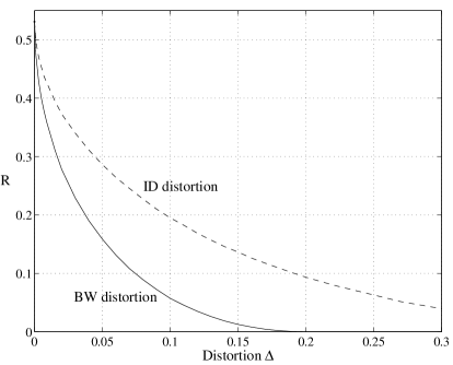
Figure 4: Rate distortion function for a visible source.

Consider next the hidden source case (or blind case) where $V=Z$. We thus have

$$R(\Delta)=\min_{\Let@\restore@math@cr\default@tag\vbox{\halign{\hfil$\m@th\scriptstyle{#}$\hfil\cr P_{Y|Z}:\\ d(P_{XY})\leq\Delta\crcr}}}I(Z;Y)$$

Again, if $\Delta=0$ then $P_{XY}=P_{XZ}$ for both the Bhattacharyya-Wootters and the informational divergence distortion measures. Performing the optimization, we find that $R(0)$ can be a discontinuous function of $\alpha_{2}$; for $\alpha_{2}\neq\alpha_{1}$ we have $R(0)=H(Z)=h(p\,\alpha_{1}+(1-p)\,\alpha_{2})$ and for $\alpha_{2}=\alpha_{1}$ we have $R(0)=0$. For example, suppose that $p=1/2$ and $\alpha_{1}=1/3$. We plot $R(\Delta)$ as a function of $\alpha_{2}$ for various $\Delta$ and the Bhattacharyya-Wootters distortion measure in Fig. 5. Observe that as $\Delta\rightarrow 0$ we will have a discontinuity at $\alpha_{2}=1/3$. In practice, this discontinuity does not occur because $\Delta=0$ is impossible for finite block lengths. Furthermore, if $\Delta$ is not too small, say $\Delta=10^{-3}$, then for many $\alpha_{2}$ one can achieve substantially better compression rates than $R(0)$.

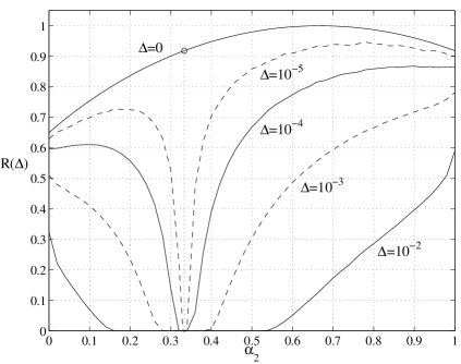
Figure 5: Rate distortion function for a hidden source.

4 Conclusions

The problem of determining optimal compression limits for quantum information has recently generated considerable interest. In the special case of an ensemble of mixed states with commuting density operators, we use rate distortion theory to find the optimal rates in both the visible and blind versions of the problem. We also generalize this special case of the quantum compression problem to the setting where the reconstruction is not faithful.

References

- [1] C. E. Shannon, “A mathematical theory of communication,” Bell System Tech. J. 27, 379-423, 623-656, 1948.
- [2] C. H. Bennett and P. W. Shor, “Quantum information theory,” I.E.E.E. Trans. Inform. Theory 44, 2724-2742, 1998.
- [3] C. E. Shannon, “Coding theorems for a discrete source with a fidelity criterion,” I.R.E. National Convention Record Part 4, 142-163, 1959.
- [4] J. Preskill, http://www.theory.caltech.edu/people/preskill/ph229/#lecture.
- [5] B. W. Schumacher, “Quantum coding,” Phys. Rev. A 51, 2738-2747, 1995.
- [6] R. Jozsa and B. W. Schumacher, “A new proof of the quantum noiseless coding theorem,” J. Modern Optics 41, 2343-2349, 1994.
- [7] H. Barnum, C. A. Fuchs, R. Jozsa, and B. Schumacher, “General fidelity limits for quantum channels,” Phys. Rev. A 54, 4707, 1996.
- [8] R. Jozsa, “Quantum noiseless coding of mixed states,” Talk given at the Third Santa Fe workshop on Complexity, Entropy, and the Physics of Information, May 1994.
- [9] M. Horodecki, “Limits for compression of quantum information carried by ensembles of mixed states,” Phys. Rev. A 57, 3364-3369, 1998.
- [10] M. Horodecki, “Towards optimal compression for mixed signal states,” LANL ArXiV.org e-print quant-ph/9905058, 1999.
- [11] H. Barnum, C. M. Caves, C. A. Fuchs, R. Jozsa, and B. Schumacher, “On quantum coding for ensembles of mixed states,” LANL ArXiV.org e-print quant-ph/0008024, August 2000.
- [12] W. Dür, G. Vidal, and J. I. Cirac, “Visible compression of commuting density operators,” to appear in LANL ArXiV.org.
- [13] T. M. Cover and J. A. Thomas, Elements of Information Theory, Wiley, New York 1991.
- [14] T. Berger, Rate Distortion Theory: A Mathematical Basis for Data Compression, Prentice-Hall, New Jersey 1971.
- [15] R. L. Dobrushin and B. S. Tsybakov, “Information transmission with additional noise,” I.E.E.E. Trans. Inform. Theory 8, 293-304, 1962.
- [16] I. Csiszár and J. Körner, Information Theory, Coding Theorems for Discrete Memoryless Systems, Akadémiai Kiadó, Budapest 1981.
- [17] R.G. Gallager, Discrete Stochastic Processes, Kluwer, Boston 1996.
- [18] R. G. Gallager, Information Theory and Reliable Communication, Wiley, New York 1968.