Reducing the Linewidth of an Atom Laser by Feedback

Abstract

A continuous atom laser will almost certainly have a linewidth dominated by the effect of the atomic interaction energy, which turns fluctuations in the condensate atom number into fluctuations in the condensate frequency. These correlated fluctuations mean that information about the atom number could be used to reduce the frequency fluctuations, by controlling a spatially uniform potential. We show that feedback based on a physically reasonable quantum non-demolition measurement of the atom number of the condensate in situ can reduce the linewidth enormously.

An atom laser is a continuous source of coherent atom waves, analogous to an ordinary laser which is a continuous source of coherent photon waves (light) [2, 3]. Ideas for creating an atom laser were published independently by a number of authors [4, 5, 6, 7], shortly after the first achievement of Bose-Einstein condensation (BEC) of gaseous atoms [8, 9, 10]. There have since been some important advances in the coherent release of pulses [11, 12] and beams [13, 14] of atoms from a condensate. Since the condensate is not replenished in these experiments, the output coupling cannot continue indefinitely [15]. Nevertheless they represent major steps towards achieving a continuously operating atom laser.

The coherence of an atom laser beam can be defined analogously to that of an optical laser beam: the atoms should have a relatively small longitudinal momentum spread, they should ideally be restricted to a single transverse mode and internal state, and their flux should be relatively constant [3]. A fourth condition, rarely considered for optical lasers because it is so easily satisfied, is that the laser beam be Bose degenerate. This requires that the atom flux be much larger than the linewidth (the reciprocal of the coherence time) [3]. A crucial contributor to the linewidth of an atom laser is the collisional interaction of atoms, which is negligible for photons. This is difficult to avoid because it is the collisions between atoms that enables BEC by evaporative cooling, at present the only method for achieving an atom laser.

In this Letter we show that using a feedback mechanism can reduce the effect of atomic interactions on the atom laser linewidth by a factor as large as the square root of the atom number. For a single-mode condensate the dominant effect of collisions is to turn atom number fluctuations in the condensate into fluctuations in the energy, which are equivalent to frequency fluctuations. By monitoring the number fluctuations, it is possible using feedback to largely compensate for the linewidth caused by these frequency fluctuations. The key practical points are that the measurement does not rely upon any external condensate phase reference, and that the control requires only the ability to change the energy of the atoms, which could be done with a spatially uniform optical or magnetic field.

We begin by deriving the standard laser linewidth (for non-interacting bosons) using a simple method which is applied to all later cases. We then derive the broadened linewidth for an atom laser with strongly interacting atoms. Finally, we show that feedback based on a quantum non-demolition (QND) measurement of atom number in the the condensate can greatly mitigate this linewidth broadening.

(a) Standard Laser Linewidth. To derive the standard linewidth we use the usual single-mode model of the laser [16, 17]. Far above threshold, the laser mode has Poissonian number statistics. In the absence of thermal or other excess noise, its dynamics are modeled by the completely positive master equation [18, 19]

$$\dot{\rho}=\kappa\mu{\cal D}[a^{\dagger}]{\cal A}[a^{\dagger}]^{-1}\rho+\kappa{\cal D}[a]\rho.$$ (1)

Here $\kappa$ is the loss rate, $\mu\gg 1$ the stationary mean boson number, and $a$ the annihilation operator for the laser mode. The superoperators ${\cal D}$ and ${\cal A}$ are defined as usual:

$${\cal D}[A]B \equiv ABA^{\dagger}-{\cal A}[A]B,$$ (2)

$${\cal A}[A]B \equiv (A^{\dagger}AB+BA^{\dagger}A)/2.$$ (3)

That Eq. (1) is of the Lindblad form follows from the identity [3, 18] ${\cal D}[a^{\dagger}]{\cal A}[a^{\dagger}]^{-1}=\int_{0}^{\infty}dq{\cal D}[a^{\dagger}e^{-qaa^{\dagger}/2}]$. The stationary solution to this master equation is

$$\rho_{\rm ss}=e^{-\mu}\sum_{n}\frac{\mu^{n}}{n!}|{n}\rangle\langle{n}|=\frac{1}{2\pi}\int_{0}^{2\pi}d\theta|{re^{i\theta}}\rangle\langle{re^{i\theta}}|,$$ (4)

where $r=\sqrt{\mu}$ and $|{re^{i\theta}}\rangle$ is a coherent state [16, 17].

The coherence time of a laser is roughly the time for the phase of the field to become uncorrelated with its initial value. It is determined by the stationary first-order coherence function

$$g^{(1)}(t)={{\rm Tr}[a^{\dagger}e^{{\cal L}t}a\rho_{\rm ss}]}/{{\rm Tr}[\rho_{\rm ss}a^{\dagger}a]}.$$ (5)

A simple and useful definition is [3]

$$\tau_{\rm coh}=\frac{1}{2}\int_{0}^{\infty}|g^{(1)}(t)|dt.$$ (6)

Here the $1/2$ is so that, for the standard laser, $\ell\equiv\tau_{\rm coh}^{-1}$ will be the standard linewidth. In the cases we consider it is a very good approximation [20] to put $|g^{(1)}(t)|=e^{-i\omega_{0}t}g^{(1)}(t)$ for some frequency $\omega_{0}$. From Eq. (5), this allows the integral in Eq. (6) to be evaluated, yielding

$$\tau_{\rm coh}\simeq-{{\rm Tr}[a^{\dagger}({\cal L}-i\omega_{0})^{-1}a\rho_{\rm ss}]}/{2{\rm Tr}[\rho_{\rm ss}a^{\dagger}a]}.$$ (7)

Equation (7) can be evaluated numerically, for example using the Matlab quantum optics toolbox [21]. Analytically, it is easier to use the fact that Eq. (5) is unchanged if $\rho_{\rm ss}$ is replaced by the coherent state $|{re^{i\theta}}\rangle\langle{re^{i\theta}}|$ for arbitrary $\theta$. Using any suitable phase-space $(\alpha,\alpha^{*})$ representation, the coherence function then becomes $g^{(1)}(t)=\left\langle{\alpha^{*}(t)}\right\rangle/\left\langle{\alpha^{*}(0)}\right\rangle$, where $\alpha(0)$ has a distribution corresponding to $|{re^{i\theta}}\rangle$. Because fluctuations in the intensity $n=|\alpha|^{2}$ are relatively small in a laser with $\mu\gg 1$, the coherence time is well approximated by

$$\tau_{\rm coh}\simeq\frac{1}{2}\int_{0}^{\infty}|\langle e^{-i\delta{\phi}(t)}\rangle|dt\simeq\frac{1}{2}\int_{0}^{\infty}e^{-\frac{1}{2}\delta V_{\phi}(t)}dt.$$ (8)

Here $\delta V_{\phi}(t)$ is the variance of $\delta\phi(t)=\arg[\alpha(t)/\alpha(0)]$, and the second approximation relies on $\delta\phi(t)$ having Gaussian statistics, as will be justified below.

For our laser model, the $Q$-function is the most convenient representation because of the identity

$${\cal D}[a^{\dagger}]{\cal A}[a^{\dagger}]^{-1}\rho\to\sum_{k=1}^{\infty}\left(\frac{-\partial}{\partial n}\right)^{k}Q(n,\phi),$$ (9)

which, since the higher order derivatives are negligible, can be truncated at $k=2$. The master equation (1) thus turns into a Fokker-Planck equation (FPE) for $Q(n,\phi)$ which can be linearized. Under this FPE, the number statistics remain those of the initial coherent state, as does the number-phase covariance $C_{n\phi}$ (i.e. it remains zero), and the phase has Gaussian statistics with a variances that increases as $\delta V_{\phi}(t)=({\kappa}/{2\mu})t$. Substituting this into Eq. (8), we obtain $\tau={2\mu}/{\kappa}$. This time is precisely the coherence time. Its reciprocal is the standard laser linewidth $\ell_{0}=\kappa/2\mu$ [16, 17, 18, 19].

(b) Atom Laser Linewidth. As a model for an atom laser we take the standard laser master equation (1) and add a term $-iC[a^{\dagger}a^{\dagger}aa,\rho]$. This represents the self-energy of the atoms due to collisions, where

$$C=\frac{2\pi\hbar a_{s}}{m}\int d^{3}{\bf r}|\psi({\bf r})|^{4}.$$ (10)

Here $\psi({\bf r})$ is the wavefunction for the condensate mode, and $a_{s}$ is the $s$-wave scattering length. For the experiments in Refs.  [11, 12, 13, 14], $\psi({\bf r})$ can be determined using the Thomas-Fermi approximation, and we use this to obtain the numerical values which appear later. The Hamiltonian $Ca^{\dagger}a^{\dagger}aa$ has no effect on the atom number statistics. Linearizing the resultant FPE for the $Q$ function yields the phase-related second-order moments

$$C_{n\phi}(t) = \frac{\chi}{2}(e^{-\kappa t}-1),$$ (11)

$$\delta V_{\phi}(t) = \frac{\chi^{2}}{2\mu}(e^{-\kappa t}+\kappa t-1)+\frac{\kappa}{2\mu}t.$$ (12)

Here, we have used $\chi=4\mu C/\kappa$ as a dimensionless parameter for the strength of the atomic interactions.

This expression for $\delta V_{\phi}(t)$ implies that the integrand $g^{(1)}(t)$ in Eq. (8) has the same structure as the analogous expression, Eq. (184), derived in Ref. [22]. This was for a condensate in dynamical equilibrium with thermal atoms. Moreover, the three time scales identified in Ref. [22] have the same physical origins as those in Eq. (12). The integral in Eq. (8) can be evaluated analytically in two limits:

$$\ell=\tau^{-1}=\left\{\begin{array}[]{lll}\kappa(1+\chi^{2})/2\mu&{\rm for}&\chi\ll\sqrt{\mu}\\ 2\kappa\chi/\sqrt{2\pi\mu}&{\rm for}&\chi\gg\sqrt{\mu}\end{array}\right..$$ (13)

These correspond to the characteristic time constants of Eqs. (187) and (186) of Ref. [22] respectively (see Ref. [23] for a further discussion). Our two expressions agree at $\chi\simeq\sqrt{8\mu/\pi}$, so we have an expression for how $\ell$ scales for all values of $\chi$. The second expression for $\tau$, in the regime where the nonlinearity is dominant, is familiar as the collapse time of an initial coherent state in the absence of pumping or damping [24, 25].

Using the preliminary atom laser experiments [11, 12, 13, 14] as a guide to realistic parameter values, the dimensionless interaction strength $\chi$ is found to always satisfy $\chi\gg 1$. This implies a linewidth for the atom laser far above the standard limit. If $\chi\gtrsim\mu^{3/2}$, then $\ell$ would be larger than the output flux $\kappa\mu$, and the output would cease to be coherent. It is thus of great interest to find methods for reducing the linewidth due to atomic interactions.

(c) Effect of QND-based Feedback. Atomic interactions do not directly cause phase diffusion. Rather, they cause a shearing of the field in phase space, with higher amplitude fields having higher energy and hence rotating faster. The linewidth-broadening which results is a known effect for optical lasers with a Kerr ($\chi^{(3)}$) medium [26]. The shearing of the field is manifest in the finite value acquired by the covariance $C_{n\phi}(t)$ in Eq. (11). It means that information about the condensate number is also information about the condensate phase. Hence, we can expect that feedback based on atom number measurements could enable the phase dynamics to be controlled, and the linewidth reduced.

It might be thought that one could measure the atom number by diverting some of the atom laser output beam. It turns out that this sort of measurement is effectively useless for reducing the linewidth. For this reason we consider instead quantum non-demolition (QND) measurements of atom number, which works very well [27].

QND atom number measurements can be performed on the condensate in situ using dispersive imaging techniques [29]. We consider a far-detuned probe laser beam of frequency $\omega_{p}$ and cross-sectional area $A$ (assumed larger than the condensate) which passes through the condensate. For simplicity, we will assume that the distortion of the beam front, and the mean phase shift, are removed by a suitable “anti-mean-condensate” lens. For a single atom, the interaction Hamiltonian with the probe beam in the large detuning limit is

$$\hbar\frac{\Omega_{p}^{2}}{4\Delta}=\hbar b^{\dagger}b\left(\frac{\hbar\omega_{p}\Gamma^{2}}{8A\Delta I_{\rm sat}}\right)\equiv\hbar b^{\dagger}b\theta,$$ (14)

where $\Omega_{p}$, $\Delta$, $\Gamma$ and $I_{\rm sat}$ have their usual meaning. Here $b$ is the annihilation operator for the probe beam, normalized so that $\hbar\omega_{p}b^{\dagger}b$ is the beam power. The effective interaction Hamiltonian for the whole condensate, minus the mean phase shift, is thus

$$H_{\rm int}=\hbar\theta(a^{\dagger}a-\mu)b^{\dagger}b,$$ (15)

where $\theta$, defined in Eq. (14), is the phase shift of the probe field due to a single atom.

From Eq. (15), the back-action of the probe fluctuations on the condensate can be evaluated using the techniques of Ref. [30], and results in the extra phase diffusion

$$\dot{\rho}=\beta^{2}{\cal D}[e^{-i\theta(a^{\dagger}a-\mu)}]\rho\simeq N{\cal D}[a^{\dagger}a]\rho.$$ (16)

Here the approximation requires $\sqrt{\mu}\theta\ll 1$, and

$$N=\beta^{2}\theta^{2}=P\theta^{2}/\hbar\omega_{p},$$ (17)

where $\beta=\left\langle{b_{\rm in}}\right\rangle$ and $P$ is the mean beam power. Equation (15) also gives the output probe field [30]

$$b_{\rm out}=e^{-i\theta(a^{\dagger}a-\mu)}b_{\rm in}\simeq b_{\rm in}-i\theta(a^{\dagger}a-\mu)\beta,$$ (18)

where the same approximation has been used. The condensate number fluctuations can thus be measured by homodyne detection of the output phase quadrature

$$I^{\rm Y}_{\rm out}=-ib_{\rm out}+ib_{\rm out}^{\dagger}\simeq I^{\rm Y}_{\rm in}-2\beta\theta(a^{\dagger}a-\mu).$$ (19)

In order to control the phase dynamics of the condensate, we wish to use the homodyne current to modulate the phase. This can be done, for example, by applying a uniform magnetic field or far-detuned light field across the whole condensate. We model this by the Hamiltonian

$$H_{\rm fb}(t)=-\hbar a^{\dagger}a\sqrt{\frac{\kappa\lambda}{4\mu}}\int_{0}^{\infty}h(s)I_{\rm out}^{\rm Y}(t-s)ds,$$ (20)

where $h(s)$ is the response function of the feedback loop and $\lambda$ is a dimensionless measure of the feedback strength. Neither the measurement nor the feedback affect the atom number statistics. In the ideal limit of instantaneous feedback, $h(s)\to\delta(s)$ and we can apply the Markovian theory of Ref. [30]. The total master equation for the atom laser is then

$$\dot{\rho} = \kappa\mu{\cal D}[a^{\dagger}]{\cal A}[a^{\dagger}]^{-1}\rho+\kappa{\cal D}[a]\rho-iC[a^{\dagger}a^{\dagger}aa,\rho]$$ (22)

$${+}\,iN\sqrt{\frac{\lambda}{\nu}}[a^{\dagger}a^{\dagger}aa,\rho]+N\left(1+\frac{\lambda}{\eta\nu}\right){\cal D}[a^{\dagger}a]\rho.$$

Here we have allowed for a detection efficiency $\eta$ [30], and dropped terms corresponding to a frequency shift, and defined a dimensionless parameter $\nu=4\mu N/\kappa$.

Proceeding as before, we find the $Q$ phase variance:

$$\delta V_{\phi}(t) = \frac{1}{2\mu}\left(\chi-\sqrt{\nu\lambda}\right)^{2}(e^{-\kappa t}+\kappa t-1)$$ (24)

$${+}\,\frac{1}{4\mu}\left(2+\nu+\frac{\lambda}{\eta}\right)\kappa t.$$

If the feedback is to reduce the linewidth, we need $(\chi-\sqrt{\lambda\nu})^{2}\ll 4\mu$ and $\eta$ must be large enough that $\eta\mu\gg 1$. In this case, Eq. (8) has a simple analytical solution:

$$\ell=\tau^{-1}=\frac{\kappa}{4\mu}\left[2+\nu+\frac{\lambda}{\eta}+2\left(\chi-\sqrt{\nu\lambda}\right)^{2}\right].$$ (25)

Assume $\chi$ is large enough that $2\sqrt{\eta}\chi>1$, which is the physically interesting regime where the self-energy is important. Then $\ell$ is minimized for a feedback strength of $\lambda=\sqrt{\eta}\chi-1/2$, and a measurement strength of $\nu=\lambda/\eta$. The optimum linewidth in this case is

$$\ell_{\rm min}=\frac{\kappa}{2\mu}\left({1+\frac{\chi}{\sqrt{\eta}}-\frac{1}{4\eta}}\right).$$ (26)

Note that for a large interaction strength $\chi$ there is an optimum measurement strength $\nu\simeq\chi/\sqrt{\eta}$ (or equivalently $N\simeq C/\sqrt{\eta}$) independent of the output coupling rate $\kappa$. From Eq. (22) we see that this effectively cancels the self-energy term in the master equation (since $\lambda=\eta\nu$). A weak measurement will give poor information about the atom number, with a high noise-to-signal ratio. Feeding back the noisy current to counter the shearing caused by the nonlinearity will thus add large phase fluctuations to the condensate. On the other hand, if the measurement is too strong the measurement back action in the form of phase diffusion, as discussed above Eq. (17), will itself dominate the linewidth.

In Fig. 1 we plot the approximate analytical expressions for the linewidth in the absence [Eq. (13)] and presence [Eq. (26)] of feedback as a function of nonlinearity $\chi$. We also plot exact numerical results using Eq. (7), for $\mu=60$. The agreement is very good. It is evident that the QND feedback offers a linewidth much smaller than that without feedback for all values of $\chi>1/2\sqrt{\eta}$. In fact for $\chi\gg 1$ the reduction factor approaches a maximum of $\sqrt{8\mu/\pi}$. Most importantly, with feedback, the laser output remains coherent until $\chi\gtrsim\mu^{2}$, a much higher value than the $\mu^{3/2}$ which applies in the absence of feedback.

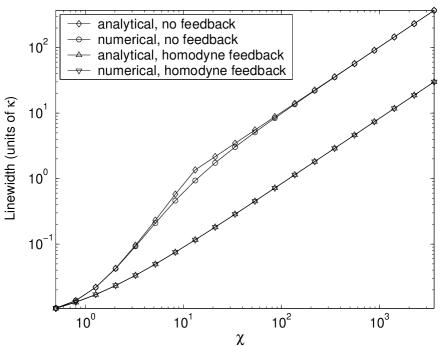
FIG. 1.: Atom laser linewidth for $\kappa=\eta=1$ and $\mu=60$, plotted with and without feedback using both analytical and numerical methods (see text).

Let us summarize. An atom laser will almost certainly suffer great linewidth broadening due to the collisional self-energy of the atoms. This is because the self-energy produces a correlation between the number and phase fluctuations of the condensate. We have shown that this broadening can be enormously reduced by controlling the phase of the condensate based on a QND measurement of the number of atoms in the condensate. The factor of reduction can be as large as the square root of the number of atoms in the condensate (that is, a factor of perhaps $10^{3}$).

A question of interest is, how easy is it to obtain a QND measurement of sufficient strength to optimize the feedback? We have seen above that we require $\nu\simeq\chi$, which is equivalent to $N\simeq C$. For the typical BEC parameters of Refs. [11, 12, 13, 14], $C\sim 10^{-2}$s^-1. It may be verified from Eq. (17) that it is very easy to obtain a measurement strength $N$ this large, even with $\Delta\gg\Gamma$.

A related question is, how much of a problem is atom loss due to spontaneous emission by atoms excited by the detuned probe beam? The rate of this loss (ignoring reabsorption) is $\Gamma\times(\textrm{Excited Population})$. We would like the ratio of this loss rate to the output loss rate $\kappa\mu$ to be small. In the $\Delta\gg\Gamma$ limit, this ratio is given by

$$\Gamma\frac{(\Gamma/2\Delta)^{2}(I/2I_{\rm sat})\mu}{\kappa\mu}\sim\frac{2\chi I_{\rm sat}A}{\hbar\omega_{p}\Gamma\mu}.$$ (27)

For physically reasonable parameters of $\chi\sim 10^{3}$, $I_{\rm sat}\sim 10$W$/$m², $A\sim 10^{-11}$m², $\omega_{p}\sim 3\times 10^{15}$s^-1, $\Gamma\sim 3\times 10^{6}$s^-1, and $\mu\sim 10^{6}$, Eq. (27) is indeed small ($\sim 10^{-1}$).

In conclusion, there appear to be no fundamental reasons that this proposal could not be put to good use when a continuous atom laser is realized.

Acknowledgments.

HMW is deeply indebted to W.D. Phillips for the idea of controlling atom laser phase fluctuations using atom number measurements, and for subsequent insightful comments on this work.

REFERENCES

- [1]
- [2] Of course, some optical lasers have a pulsed rather than continuous output. However, as argued in Ref. [3], in order for the term “atom laser” to mean something more than merely an atomic Bose-Einstein condensate released from its trap, it is useful to impose the condition that a true atom laser have a continuous output.
- [3] H.M. Wiseman, Phys. Rev. A 56, 2068 (1997).
- [4] H.M. Wiseman and M.J. Collett, Phys. Lett. A 202, 246 (1995).
- [5] R.J.C. Spreeuw, T. Pfau, U. Janicke, and M. Wilkens, Europhys. Lett. 32, 469 (1995).
- [6] M. Olshanii, Y. Castin, and J. Dalibard, in Proc. XII Conference on Lasers Spectroscopy, edited by M. Inguscio, M. Allegrini and A. Sasso (World Scientific, 1995).
- [7] M. Holland et al, Phys. Rev. A 54, R1757 (1996).
- [8] M.H. Anderson et al, Science 269, 198 (1995).
- [9] C.C Bradley, C.A. Sackett, J.J. Tollett, and R.G. Hulet, Phys. Rev. Lett. 75, 1687 (1995).
- [10] K.B. Davis et al., Phys. Rev. Lett. 75, 3969 (1995).
- [11] M.-O. Mewes, M. R. Andrews, D. M. Kurn, D. S. Durfee, C. G. Townsend, and W. Ketterle, Phys. Rev. Lett. 78, 582 (1997)
- [12] B.P. Anderson, M.A.Kasevich, Science 282, 1686 (1998).
- [13] E.W. Hagley, L. Deng, M, Kozuma, J. Wen, K. Helmerson, S.L. Rolston, W.D. Phillips, Science 283, 1706 (1999);
- [14] I. Bloch, T.W. Hänsch, and T. Esslinger Phys. Rev. Lett. 82, 3008 (1999).
- [15] In some recent experiments a large thermal cloud does replenish the condensate, but not on a continuous basis (W.D. Phillips, pers. comm.).
- [16] W.H. Louisell, Quantum Statistical Properties of Radiation (John Wiley & Sons, New York, 1973).
- [17] M. Sargent, M.O. Scully, and W.E. Lamb, Laser Physics (Addison-Wesley, Reading Mass., 1974).
- [18] H.M. Wiseman, Phys. Rev. A 47, 5180 (1993).
- [19] H.M. Wiseman, Phys. Rev. A 60, 4083 (1999).
- [20] We have shown analytically and numerically that the relative error caused by this approximation is .
- [21] S.M. Tan, J. Opt. B 1, 424 (1999).
- [22] C.W. Gardiner and P.Zoller, Phys. Rev. A 58, 536 (1998).
- [23] D. Jaksch, C.W. Gardiner, M.K. Gheri, and P. Zoller, Phys Rev A 58, 1450 (1998).
- [24] E. M. Wright, D. F. Walls, and J. C. Garrison, Phys. Rev. Lett. 77, 2158 (1996).
- [25] A. Imamolu, M. Lewenstein, and L. You, Phys. Rev. Lett. 78, 2511 (1997).
- [26] K. Watanabe et al., Phys. Rev. A 42, 5667 (1990).
- [27] This is perhaps not surprising, since feedback based on demolition photodetection cannot produce squeezed states, whereas that based on QND detection can [28]
- [28] H.M. Wiseman and G.J. Milburn, Phys. Rev. A 49, 1350 (1994).
- [29] M.R. Andrews, M.-O. Mewes, N.J. van Druten, D.S. Durfee, D.M. Kurn, and W. Ketterle, Science 273, 84 (1996).
- [30] H.M. Wiseman, Phys. Rev. A 49, 2133 (1994); Errata ibid., 49 5159 (1994) and ibid. 50, 4428 (1994).