Entanglement of transverse modes in a pendular cavity

Abstract

We study the phenomena that arise in the transverse structure of electromagnetic field impinging on a linear Fabry-Perot cavity with an oscillating end mirror. We find quantum correlations among transverse modes which can be considered as a signature of their entanglement.

I Introduction

It is now well assessed that an empty optical cavity with a moving mirror in its steady state may mimic a Kerr medium if illuminated with coherent light [1, 2]. When the mirror is free to oscillate, the radiation pressure induces a coupling between its position and the intensity of the light beam, modifying the optical path in an intensity dependent way. A wide range of applications of this effect have been recentely developed [3]. In particular the system, showing a typical bistable behaviour, can be used as a quantum noise eater device, because the output light is significantly squeezed [4, 5], or to generate highly nonclassical states for both radiation and mirror [6, 7], due to the nonlinear character of the interaction. The theoretical treatments of this model were fully quantum but at most one dimensional in space because of the plane wave approximation, which ensures that the electric field is uniform over the transverse plane. This means that the investigations dealt only with temporal-frequency aspects, neglecting all features related to space. On the other hand, recent years have seen an increasing interest towards the spatial aspects [8]. Hence, the aim of this paper is to study the spatial phenomena that arise in the transverse structure of the light field impinging on a linear Fabry-Perot cavity with an oscillating end mirror. We shall show the possibility to correlate transverse modes, other than to obtain squeezing effects. Such correlations have different nature, and could reveal entanglement [9, 10]. Moreover, we will analyse the differences and analogies with a Kerr nonlinear system, and we will investigate the influence of temperature on the transverse structures for such optomechanical system.

II The Model

We consider a linear Fabry-Perot empty cavity with one fixed mirror, partially transmitting, and one perfectly reflecting end mirror. The completely reflecting mirror, having a mass $m$, can move, back and forth along the cavity axes (say $z$), undergoing harmonic oscillations at frequency $\omega_{m}$. The amplitude of such oscillations is however, much less than the equilibrium cavity length $L$. The cavity resonances are calculated in absence of the impinging light. The characteristic cavity frequencies are assumed many orders of magnitude greater than $\omega_{m}$ to ensure that the number of photons generated by the Casimir effect is completely negligible. We also assume that the cavity round trip time is much shorter than the mirror’s period of oscillation and the Doppler frequency shift of the photons [11] on the moving mirror, is completely negligible.

A The Single Mode Model

Let us recall the model describing the system in the approximation where all the spatial effects (e.g. diffraction) are neglected and the cavity is assumed to operate in a single longitudinal mode of frequency $\omega_{0}$. That cavity mode is coherently driven by the action of an external field ${\cal E}e^{-i\omega_{s}t}$, having a frequency $\omega_{s}$ and a complex amplitude ${\cal E}$. By indicating with $A$, $A^{{\dagger}}$ the annihiliation and creation operators of the cavity mode, the system Hamiltonian, in a frame rotating at the frequency $\omega_{s}$, reads [5]

$$H=\hbar\Delta A^{{\dagger}}A+\hbar\omega_{m}\left(\frac{P^{2}_{X}}{2}+\frac{X^{2}}{2}\right)-\hbar gA^{{\dagger}}AX+i\hbar\left({\cal E}A^{{\dagger}}-{\cal E}^{*}A\right)\,,$$ (1)

where $\Delta=\omega_{0}-\omega_{s}$ is the cavity detuning; $X$ and $P_{X}$ are the dimensionless position and momentum operators of the mirror, obeying the commutation relation $[X,P_{X}]=i$. The interaction part (third term) of Eq.(1) accounts for the effect of radiation pressure force which causes the instantaneous displacement of the mirror, and the coupling constant is given by [5]

$$g=\frac{\omega_{0}}{L}\sqrt{\frac{\hbar}{m\omega_{m}}}\,.$$ (2)

In writing down the equations describing the dynamics of the system, we must take into account the damping of the movable mirror due to the coupling with a thermal bath in equilibrium at temperature $T$, and the cavity losses, due to the coupling of the internal mode with all the external modes of radiation through the fixed (transmitting) mirror. Hence, we have the following quantum Langevin equations

$$\partial_{t}\,A(t) = -i\Delta A(t)+igX(t)A(t)+{\cal E}-\gamma_{c}\,A(t)+\sqrt{2\gamma_{c}}\,A_{\rm in}(t)\,,$$ (3)

$$\partial_{t}\,X(t) = \omega_{m}P_{X}(t)\,,$$ (4)

$$\partial_{t}\,P_{X}(t) = -\omega_{m}X(t)+gA^{{\dagger}}(t)A(t)-\gamma_{m}P_{X}(t)+\sqrt{\gamma_{m}}\,\epsilon_{\rm in}(t)\,,$$ (5)

where $\gamma_{c}$, $\gamma_{m}$ are the decay rates of the cavity mode and of the mirror momentum, respectively. The noise operators (labeled with the subscript “in”) have zero expectation value, and obey the following correlations:

$$\langle A_{\rm in}(t)A_{\rm in}(t^{\prime})\rangle=0\,,\quad\langle A_{\rm in}(t)A^{{\dagger}}_{\rm in}(t^{\prime})\rangle=\delta(t-t^{\prime})\,,$$ (6)

$$\langle\epsilon_{\rm in}(t)\epsilon_{\rm in}(t^{\prime})\rangle=N_{T}\delta(t-t^{\prime})\,,$$ (7)

where $N_{T}$ is the number of thermal excitations of the mirror $N_{T}=k_{B}T/\hbar\omega_{m}$, with $k_{B}$ being the Boltzmann constant. The form of Eq.(3) with correlations (6) corresponds to the quantum optical master equation [12]. Instead, the form of Eqs.(4), (5), with correlations (7), corresponds to the standard quantum Brownian master equation [12]. The latter is only valid in the limit $N_{T}\gg 1$, while a more careful analysis is required in the opposite limit [13].

B The Spatially Multimode Model

Motivated by the recent progress in the study of transverse quantum effects in optical systems [8] we wish to extend the previous model to the case of spatially multimode fields. Let us again assume the validity of the single longitudinal mode approximation, which, toghether with the mean field approximation allows us to neglect the dependence of the field over the variable $z$. However, we now allow the radiation field to depend on the transverse vector ${\bf x}\equiv(x,y)$, which is the position vector in the plane orthogonal to the direction $z$ of propagation of fields.

Then, Eqs.(3), (4), (5) after elimination of $P_{X}$, must be rewritten as

$$\partial_{t}\,A({\bf x},t) = -i\Delta A({\bf x},t)+igX(t)A({\bf x},t)+{\cal E}({\bf x})-\gamma_{c}\,A({\bf x},t)+i\gamma_{c}\ell_{D}^{2}\nabla_{\perp}^{2}A({\bf x},t)+\sqrt{2\gamma_{c}}\,A_{\rm in}({\bf x},t)\,,$$ (8)

$$\partial_{t}^{2}\,X(t) = -\omega_{m}^{2}X(t)+g\omega_{m}\int\,d{\bf x}\,A^{{\dagger}}({\bf x},t)A({\bf x},t)-\gamma_{m}\partial_{t}X(t)+\omega_{m}\sqrt{\gamma_{m}}\,\epsilon_{\rm in}(t)\,,$$ (9)

where the transverse Laplacian $\nabla^{2}_{\perp}\equiv\partial^{2}/\partial x^{2}+\partial^{2}/\partial y^{2}$ has been introduced to describe the diffraction in the paraxial approximation [14]. The coefficient $\ell_{D}^{2}$ has the dimension of an area, and is given by $\ell_{D}^{2}=c^{2}/2\omega_{s}\gamma_{c}$. It represents the typical length scale for spatial structures emerging in an optical resonators. In the following we shall rescale all the spatial lengths over $\ell_{D}$.

For the sake of simplicity we considered only the case of a uniform mirror motion over the transverse plane, even if there is the possibility to take into account acoustic modes of the resonators [15], but this is planned for a future work.

In order to avoid difficulties arising from the continuum of transverse modes, we consider in the transverse plane $(x,y)$ a square of side $\ell$, and we assume periodic boundary conditions for the fields. A complete set of transverse modes (corresponding to a single longitudinal resonance) is then given by

$$f_{\bf n}({\bf x})=\frac{1}{\ell}\exp\left(i{\bf k}_{\bf n}\cdot{\bf x}\right)\,,\quad{\rm with}\quad{\bf k}_{\bf n}=\frac{2\pi}{\ell}{\bf n}\,,\quad{\bf n}\equiv(n_{x},n_{y})\,,$$ (10)

where $(n_{x},n_{y})$ is a couple of integer numbers, $n_{x},n_{y}=0,\pm 1,\pm 2\ldots$. Then, the fields can be expanded in the following way

$$A({\bf x},t) = \sum_{{\bf n}}f_{\bf n}({\bf x})a_{{\bf n}}(t)=\frac{1}{\ell}\sum_{{\bf n}}e^{i{\bf k}_{\bf n}\cdot{\bf x}}a_{{\bf n}}(t)\,,$$ (11)

$${\cal E}({\bf x}) = \sum_{{\bf n}}f_{\bf n}({\bf x})e_{{\bf n}}=\frac{1}{\ell}\sum_{{\bf n}}e^{i{\bf k}_{\bf n}\cdot{\bf x}}e_{{\bf n}}\,.$$ (12)

The Hamiltonian (1) of the single mode model can thus be generalized as

$$H=\hbar\omega_{m}\left(\frac{P^{2}_{X}}{2}+\frac{X^{2}}{2}\right)+\sum_{{\bf n}}\left[\hbar\Delta_{{\bf n}}a^{{\dagger}}_{{\bf n}}a_{{\bf n}}\right]-\hbar g\sum_{{\bf n}}\left[a^{{\dagger}}_{{\bf n}}a_{{\bf n}}X\right]+i\hbar\sum_{{\bf n}}\left[a^{{\dagger}}_{{\bf n}}e_{{\bf n}}-a_{{\bf n}}e^{*}_{{\bf n}}\right]\,,$$ (13)

where we introduced the mode detuning $\Delta_{\bf n}=\omega_{\bf n}-\omega_{s}$, with

$$\omega_{{\bf n}}=\omega_{0}+\gamma_{c}{\bf k}^{2}_{{\bf n}}\,,$$ (14)

the frequency of the transverse mode ${\bf n}$.

We are now able to derive from Eq.(13) the Langevin equation for each transverse mode

$$\partial_{t}\,a_{\bf n}(t) = -i\Delta_{\bf n}a_{\bf n}(t)+igX(t)a_{\bf n}(t)+e_{\bf n}(t)-a_{\bf n}(t)+\sqrt{2}\,a_{\bf n}^{\rm in}(t)\,,$$ (15)

$$\partial_{t}^{2}\,X(t) = -\omega_{m}^{2}X(t)+g\omega_{m}\sum_{\bf m}a^{{\dagger}}_{\bf m}(t)a_{\bf m}(t)-\gamma_{m}\partial_{t}X(t)+\omega_{m}\sqrt{\gamma_{m}}\,\epsilon_{\rm in}(t)\,,$$ (16)

where we introduced the following scalings

$$\gamma_{c}t\to t\,,\;\;\omega_{m}/\gamma_{c}\to\omega_{m}\,,\;\;\gamma_{m}/\gamma_{c}\to\gamma_{m}\,,\;\;g/\gamma_{c}\to g\,,\;\;{\cal E}/\gamma_{c}\to{\cal E}\,,\;\;\Delta_{\bf n}/\gamma_{c}\to\Delta_{\bf n}\,,\;\;A_{\rm in}/\sqrt{\gamma_{c}}\to A_{\rm in}\,,\;\;\epsilon_{\rm in}/\sqrt{\gamma_{c}}\to\epsilon_{\rm in}\,.$$

Equations (15), (16) show that each mode interacts with the mirror, which in turn becomes an intermediary between the various modes, redistributing the quantum information among them. Depending on such a process we expect that the output light will have different characteristics from the input one.

III The Steady State

We are actually interested in the classical steady state regime and in small fluctuations around this steady state. To this end, as it is usually in the semiclassical treatment of quantum noise, we set $a_{\bf n}=\alpha_{\bf n}+\delta a_{\bf n}$, $X=x+\delta X$, where the c-numbers $\alpha_{\bf n}$, $x$ are solutions of the classical steady state equations

$$0 = -i\Delta_{{\bf n}}\alpha_{{\bf n}}+igx\alpha_{{\bf n}}+e_{{\bf n}}-\alpha_{{\bf n}}\,,$$ (17)

$$0 = -\omega_{m}^{2}x+g\omega_{m}\sum_{{\bf m}}\left|\alpha_{{\bf m}}\right|^{2}\,,$$ (18)

By eliminating the variable $x$ from Eqs.(17), (18), it is possible to get an infinite set of coupled cubic equations

$$e_{\bf n}=\alpha_{\bf n}\left\{1+i\left[\sum_{\bf m}\left|\alpha_{\bf m}\right|^{2}-\Delta_{\bf n}\right]\right\}\,,$$ (19)

where we have scaled the variables as follows

$$\left(\frac{g^{2}}{\omega_{m}}\right)^{1/2}\alpha_{\bf n}\to\alpha_{\bf n}\,,\quad\left(\frac{g^{2}}{\omega_{m}}\right)^{1/2}e_{\bf n}\to e_{\bf n}\,.$$ (20)

In the case of only one spatial mode, the above set of equations reduces to only one cubic equation which shows a typical bistable behavior [5].

To proceede on we consider, without loss of generality, a gaussian and real pump

$${\cal E}({\bf x}\,)=\sqrt{\frac{2}{\pi}}\frac{{\cal E}}{w_{p}}e^{-(x^{2}+y^{2})/w_{p}^{2}}\,,$$ (21)

where $w_{p}$ idicates the pump waist (we will always use $\ell\gg w_{p}$). The total input power is given by

$$P_{\rm in}={\cal E}^{2}=\int\,d{\bf x}\,|{\cal E}({\bf x}\,)|^{2}\,,$$ (22)

while the pump components on the spatial modes are

$$e_{\bf n}={\cal E}\frac{\sqrt{2\pi}w_{p}}{\ell}\exp\left[-\left(\frac{w_{p}}{2}\right)^{2}{\bf k}_{\bf n}^{2}\right]\,.$$ (23)

Now, by defining the intracavity power $P$ as

$$P=\int\,d{\bf x}\,|\alpha({\bf x}\,)|^{2}=\sum_{\bf n}|\alpha_{\bf n}|^{2}\,,$$ (24)

from Eq. (19) we can obtain

$$|\alpha_{\bf n}|^{2}=\frac{|e_{\bf n}|^{2}}{1+(P-\Delta_{\bf n})^{2}}\,,$$ (25)

and summing over the index ${\bf n}$

$$P_{\rm in}=P\left\{\sum_{\bf n}\frac{2\pi\left(\frac{w_{p}}{\ell}\right)^{2}\exp\left[-\left(\frac{w_{p}^{2}}{2}\right){\bf k}_{\bf n}^{2}\right]}{1+\left[\Delta_{\bf n}-P\right]^{2}}\right\}^{-1}\,.$$ (26)

This equation gives the functional relation between the incident and intracavity intensity. The bistable behavior for the total intensity is shown in Fig.1. Depending on the slope of the curve, we have stable and unstable branches. Once one has choosen the working point along this curve, the input and intracavity powers are well defined, hence it is possible to calculate each single steady state components of the intracavity field as

$$\alpha_{\bf n}=\sqrt{P_{\rm in}}\frac{\sqrt{2\pi}\left(\frac{w_{p}}{\ell}\right)\exp\left[-\left(\frac{w_{p}}{2}\right)^{2}{\bf k}_{\bf n}^{2}\right]}{1+i\left[\Delta_{\bf n}-P\right]}\,.$$ (27)

By considering also the field reflected at the transmitting mirror we have the input-output relation [16], in terms of scaled variables

$$\alpha_{\rm out}({\bf x})=2\alpha({\bf x})-\alpha_{\rm in}({\bf x})\,,$$ (28)

where ${\cal E}({\bf x})\equiv\alpha_{\rm in}({\bf x})$. It is possible to see, in Fig. 2, that the Gaussian profile of the beam is maintained from input to outgoing fields.

Finally, the stationary displacement of the mirror due to the radiation pressure results $x=P/g$.

IV Dynamics of Small Fluctuations

The evolution equations for small fluctuations coming from the linearization of the Eqs.(15), (16) around a stable steady state are

$$\partial_{t}\,\delta a_{\bf n}(t) = -i\Delta_{\bf n}\delta a_{\bf n}(t)+i\sqrt{\omega_{m}}\delta X(t)\alpha_{\bf n}+iP\,\delta a_{\bf n}(t)-\delta a_{\bf n}(t)+\sqrt{2}\,\delta a_{\bf n}^{\rm in}(t)\,,$$ (29)

$$\partial_{t}^{2}\,\delta X(t) = -\omega_{m}^{2}\delta X(t)+\omega_{m}\sqrt{\omega_{m}}\sum_{\bf m}\left[\alpha_{\bf m}\delta a^{{\dagger}}_{\bf m}(t)+\alpha^{*}_{\bf m}\delta a_{\bf m}(t)\right]-\gamma_{m}\partial_{t}\delta X(t)+\omega_{m}\sqrt{\gamma_{m}}\,\epsilon_{\rm in}(t)\,.$$ (30)

We immediately recognize that in the case of flat pump, i.e. $\alpha_{{\bf n}}=\alpha_{{\bf 0}}\,\delta_{{\bf n},{\bf 0}}$, the coupling with the mirror occours only for one mode (the fundamental), hence no transverse effects can arise. This is one of the peculiar differences with respect to the Kerr-like model, and it is due to the fact that only one mode practically survive at steady state.

In the frequency domain Eqs.(29), (30) become

$$i\Omega\,\delta{\tilde{a}}_{{\bf n}}(\Omega) = -i\Delta_{{\bf n}}\delta{\tilde{a}}_{{\bf n}}(\Omega)+i\sqrt{\omega_{m}}\delta{\tilde{X}}(\Omega)\alpha_{{\bf n}}+iP\,\delta{\tilde{a}}_{{\bf n}}(\Omega)-\delta{\tilde{a}}_{{\bf n}}(\Omega)+\sqrt{2}\,\delta{\tilde{a}}_{{\bf n}}^{{\rm in}}(\Omega)\,,$$ (31)

$$-\Omega^{2}\,\delta{\tilde{X}}(\Omega) = -\omega_{m}^{2}\delta{\tilde{X}}(\Omega)+\omega_{m}\sqrt{\omega_{m}}\sum_{{\bf k}}\left[\alpha_{{\bf k}}\delta{\tilde{a}}^{{\dagger}}_{{\bf k}}(-\Omega)+\alpha^{*}_{{\bf k}}\delta{\tilde{a}}_{{\bf k}}(\Omega)\right]-i\Omega\gamma_{m}\delta{\tilde{X}}(\Omega)+\omega_{m}\sqrt{\gamma_{m}}\,{\tilde{\epsilon}}_{\rm in}(\Omega)\,.$$ (32)

By eliminating the mirror variables one gets an infinite set of linear equations

$$\left[i\Omega+i\Delta_{{\bf n}}-iP+1\right]\delta{\tilde{a}}_{{\bf n}}(\Omega)-i\alpha_{{\bf n}}\chi(\Omega)\sum_{\bf m}\left[\alpha_{\bf m}\delta{\tilde{a}}_{\bf m}^{{\dagger}}(-\Omega)+\alpha^{*}_{\bf m}\delta{\tilde{a}}_{\bf m}(\Omega)\right]=\sqrt{2}\,\delta{\tilde{a}}_{{\bf n}}^{{\rm in}}(\Omega)+i\alpha_{{\bf n}}\,\chi(\Omega)\sqrt{\frac{\gamma_{m}}{\omega_{m}}}\,{\tilde{\epsilon}}_{\rm in}(\Omega)\,,$$ (33)

where we have introduced the mirror response function

$$\chi(\Omega)=\frac{\omega_{m}^{2}}{\omega_{m}^{2}-\Omega^{2}+i\gamma_{m}\Omega}\,,\quad\chi^{*}(\Omega)=\chi(-\Omega)\,.$$ (34)

Other typical differences between this model and a Kerr nonlinear system are due to the dynamics of the moving mirror characterized by a frequency dependent susceptibility, and to the presence of a thermal noise as can be seen from Eqs.(34) and (7).

In Eq.(33) we may see that the various radiation modes can become correlated and some spatial effects should appear. The latter should also depend on temperature.

V Solutions

In order to find the solutions of Eqs.(33), let us write them in a matricial form. In doing so, we introduce a truncation in the number of modes effectively achieved, namely we let $n_{x},n_{y}=-{\overline{n}},\ldots,{\overline{n}}$. The truncation is reasonable given the fact that the pump field supports a finite number of modes.

Then we introduce the following vectors

$${\cal V}=\left[\begin{array}[]{c}\left(\begin{array}[]{c}\delta{\tilde{a}}_{-{\overline{n}},-{\overline{n}}}(\Omega)\\ \delta{\tilde{a}}^{{\dagger}}_{-{\overline{n}},-{\overline{n}}}(-\Omega)\end{array}\right)\\ \vdots\\ \left(\begin{array}[]{c}\delta{\tilde{a}}_{{\overline{n}},-{\overline{n}}}(\Omega)\\ \delta{\tilde{a}}^{{\dagger}}_{{\overline{n}},-{\overline{n}}}(-\Omega)\end{array}\right)\\ \vdots\\ \vdots\\ \left(\begin{array}[]{c}\delta{\tilde{a}}_{-{\overline{n}},{\overline{n}}}(\Omega)\\ \delta{\tilde{a}}^{{\dagger}}_{-{\overline{n}},{\overline{n}}}(-\Omega)\end{array}\right)\\ \vdots\\ \left(\begin{array}[]{c}\delta{\tilde{a}}_{{\overline{n}},{\overline{n}}}(\Omega)\\ \delta{\tilde{a}}^{{\dagger}}_{{\overline{n}},{\overline{n}}}(-\Omega)\end{array}\right)\end{array}\right]\,,\quad{\cal A}=\left[\begin{array}[]{c}\left(\begin{array}[]{c}i\alpha_{-{\overline{n}},-{\overline{n}}}\\ -i\alpha^{*}_{-{\overline{n}},-{\overline{n}}}\end{array}\right)\\ \vdots\\ \left(\begin{array}[]{c}i\alpha_{{\overline{n}},-{\overline{n}}}\\ -i\alpha^{*}_{{\overline{n}},-{\overline{n}}}\end{array}\right)\\ \vdots\\ \vdots\\ \left(\begin{array}[]{c}i\alpha_{-{\overline{n}},{\overline{n}}}\\ -i\alpha^{*}_{-{\overline{n}},{\overline{n}}}\end{array}\right)\\ \vdots\\ \left(\begin{array}[]{c}i\alpha_{{\overline{n}},{\overline{n}}}\\ -i\alpha^{*}_{{\overline{n}},{\overline{n}}}\end{array}\right)\end{array}\right]\,,\quad{\cal D}=\left[\begin{array}[]{c}\left(\begin{array}[]{c}\Delta_{-{\overline{n}},-{\overline{n}}}\\ \Delta_{-{\overline{n}},-{\overline{n}}}\end{array}\right)\\ \vdots\\ \left(\begin{array}[]{c}\Delta_{{\overline{n}},-{\overline{n}}}\\ \Delta_{{\overline{n}},-{\overline{n}}}\end{array}\right)\\ \vdots\\ \vdots\\ \left(\begin{array}[]{c}\Delta_{-{\overline{n}},{\overline{n}}}\\ \Delta_{-{\overline{n}},{\overline{n}}}\end{array}\right)\\ \vdots\\ \left(\begin{array}[]{c}\Delta_{{\overline{n}},{\overline{n}}}\\ \Delta_{{\overline{n}},{\overline{n}}}\end{array}\right)\end{array}\right]\,.$$ (83)

They all have $2(2{\overline{n}}+1)^{2}$ components.

Now, the system of Eqs.(33), can be written as

$$\left[{\cal M}+\left(i\Omega+1\right){\cal I}\right]\cdot{\cal V}=\sqrt{2}\,{\cal V}^{\rm in}+\sqrt{\frac{\gamma_{m}}{\omega_{m}}}\chi(\Omega){\cal A}\,{\tilde{\epsilon}}_{\rm in}(\Omega)\,,$$ (84)

where the vector ${\cal V}^{\rm in}$ is defined analogously to Eq.(83), but for the input operators. Instead, ${\cal I}$ is the $2(2{\overline{n}}+1)^{2}\times 2(2{\overline{n}}+1)^{2}$ identity matrix, while ${\cal M}$ is the $2(2{\overline{n}}+1)^{2}\times 2(2{\overline{n}}+1)^{2}$ matrix given by

$${\cal M}_{k,l}=i(-)^{k}\left[P-{\cal D}_{k}\right]\delta_{k,l}+i(-)^{l}\,\chi(\Omega)\,{\cal A}_{k}\,{\cal A}_{l-(-1)^{l}}\,,$$ (85)

By inverting the relation (84) we can get the formal solution of the system as

$${\cal V}={\cal F}\cdot\left[\sqrt{2}\,{\cal V}_{\rm in}+\sqrt{\frac{\gamma_{m}}{\omega_{m}}}\chi(\Omega){\cal A}\,{\tilde{\epsilon}}_{\rm in}(\Omega)\right]\,,\qquad{\cal F}=\left[{\cal M}+\left(i\Omega+1\right){\cal I}\right]^{-1}\,.$$ (86)

However we are looking for the solution of the outgoing modes. Then, the input-output relation [16] can be written in vector form as

$${\cal V}^{\rm out}=\sqrt{2}\,{\cal V}-{\cal V}^{\rm in}\,,$$ (87)

and if we combine it with Eq.(86), we get

$${\cal V}^{\rm out}={\cal B}\cdot{\cal V}^{\rm in}+{\cal U}{\tilde{\epsilon}}_{\rm in}\,,$$ (88)

where

$${\cal B}=2\,{\cal F}-{\cal I}\,,$$ (89)

and

$${\cal U}=\sqrt{2\frac{\gamma_{m}}{\omega_{m}}}\,\chi(\Omega)\,{\cal F}\cdot{\cal A}\,.$$ (90)

From the above matrix relations one can extract the expression for the various components $\delta{\tilde{a}}^{\rm out}_{n_{x},n_{y}}(\Omega)$, $\delta{\tilde{a}}^{{\rm out}\,{\dagger}}_{n_{x},n_{y}}(\Omega)$ in terms of the input noise operators.

Finally, it is worth noting that the transformation among input and output fields could not preserve the commutation relations. This can be understand by observing Eq.(85) where ${\rm Re}\{{\cal M}_{k,k}\}$ yields and additional damping term $\gamma_{\rm add}\propto{\rm Im}\{\chi(\Omega)\}$. Neverthless, if $\gamma_{\rm add}\ll 1$ the commutation relations are preserved. That happen for istance in the case of $\Omega\to 0$.

VI The Output Correlations

Using Eq.(7), and the fact that all the elements of the vector ${\cal V}^{\rm in}$ are uncorrelated except those of the form

$$\langle{\cal V}^{\rm in}_{2k-1}(\Omega){\cal V}^{\rm in}_{2l}(\Omega^{\prime})\rangle=\delta\left(\Omega+\Omega^{\prime}\right)\delta_{k,l}\,,$$ (91)

we are able to calculate the correlations of the output modes from the components of Eq.(88). They result:

$$\langle\delta{\tilde{a}}^{{\rm out}{\dagger}}_{\bf n}(-\Omega)\delta{\tilde{a}}^{\rm out}_{\bf m}(\Omega^{\prime})\rangle=\Bigg{[}\sum_{k=1}^{(2{\overline{n}}+1)^{2}}{\cal B}_{\{{\bf n}\}+2,2k-1}\,{\cal B}_{\{{\bf n}\}+1,2k}+N_{T}\,{\cal U}_{\{{\bf n}\}+2}\,{\cal U}_{\{{\bf n}\}+1}\Bigg{]}\delta\left(\Omega+\Omega^{\prime}\right)\,,$$ (92)

and

$$\langle\delta{\tilde{a}}^{\rm out}_{\bf n}(\Omega)\delta{\tilde{a}}^{\rm out}_{\bf m}(\Omega^{\prime})\rangle=\Bigg{[}\sum_{k=1}^{(2{\overline{n}}+1)^{2}}{\cal B}_{\{{\bf n}\}+1,2k-1}\,{\cal B}_{\{{\bf n}\}+1,2k}+N_{T}\,{\cal U}_{\{{\bf n}\}+1}\,{\cal U}_{\{{\bf n}\}+1}\Bigg{]}\delta\left(\Omega+\Omega^{\prime}\right)\,,$$ (93)

where $\{{\bf n}\}\equiv 2(2{\overline{n}}+1)(n_{y}+{\overline{n}})+2(n_{x}+{\overline{n}})$.

We now introduce the linearized output intensity operator

$$\delta\,{\tilde{I}}_{\bf n}^{\rm out}(\Omega)=\alpha_{\bf n}^{{\rm out}\,*}\delta\,{\tilde{a}}_{\bf n}^{\rm out}(\Omega)+\alpha_{\bf n}^{\rm out}\delta\,{\tilde{a}}_{\bf n}^{{\rm out}\,{\dagger}}(-\Omega)\,.$$ (94)

Then, the spectrum of the output intensity correlations among the various modes, namely

$$S^{\rm out}_{{\bf n},{\bf m}}(\Omega)=\int\,d\Omega^{\prime}\;\frac{\langle\delta\,{\tilde{I}}_{\bf n}^{\rm out}(\Omega)\delta\,{\tilde{I}}_{\bf m}^{\rm out}(\Omega^{\prime})\rangle}{|\alpha_{\bf n}^{\rm out}||\alpha_{\bf m}^{\rm out}|}\,,$$ (95)

can be easily calculated by using Eqs.(92), (93). It should be compared with that of a coherent state, i.e. $S^{\rm out}_{{\bf n},{\bf m}}(\Omega)=\delta_{{\bf n},{\bf m}}$.

Furthermore, by considering the total output intensity $\delta{\tilde{I}}^{\rm out}(\Omega)=\sum_{\bf n}\delta{\tilde{I}}^{\rm out}_{\bf n}(\Omega)$, it is possible to define the output intensity spectrum

$$S^{\rm out}(\Omega)=\int\,d\Omega^{\prime}\;\frac{\langle\delta\,{\tilde{I}}^{\rm out}(\Omega)\delta\,{\tilde{I}}^{\rm out}(\Omega^{\prime})\rangle}{\sum_{\bf n}|\alpha_{\bf n}^{\rm out}|^{2}}\,,$$ (96)

which, again, can be easily calculated by using Eqs.(92), (93). It should be compared with that of a coehrent state, i.e. $S^{\rm out}(\Omega)=1$.

VII Results and Conclusions

To study numerically the system, we have considered a pump defined by ($19\times 19$) modes.

In Fig.3 we show the intensity (auto)correlation spectrum for each mode, $S^{\rm out}_{{\bf n},{\bf n}}(\Omega=0.1)$. The squeezing is found in several modes around the fundamental, but it tends to disappear when the temperature increases. The total intensity squeezing $S^{\rm out}(\Omega=0.1)$ has been calculated for the three cases of Fig.3 obtaining the following values: 0.11, 0.62, and 1.14. The order of magnitude is similar to that obtained in Refs.[4, 5], however, in this case the total squeezing is distributed among the various mode.

In Fig.4 we plot the intensity correlation spectrum of the fundamental mode with each other $S^{\rm out}_{{\bf 0},{\bf n}}(\Omega=0.1)$. At low temperature we have a negative correlation of the fundamental mode with the neighbourhoods (the central peak instead represents the autocorrelation of the fundamental mode, i.e. its intensity squeezing). The negative correlations, i.e. anticorrelations, can be understood by considering the interaction with the mirror as redistributing the photons from the fundamental (pumped) mode to its neighbourhoods. On the other hand these anticorrelations could be considered as a signature of entanglement. In fact, thought the notion of entanglement is not clear for open system, we can see from Eqs.(88), (95) that the correlations among various modes arise as consequence of both vacuum noise and thermal noise. However, the latter, which is of classsical origin, only leads to positive correlations. Instead, the vacuum noise, purely quantum, can give positive as well as negative correlations. Therefore, anticorrelations can be considered as a signature of purely quantum correlations, hence, entanglement. Nevertheless, the two types of correlations become competing as can be seen from top to bottom of Fig.4. As matter of fact, by increasing the temperature the negative correlations tend to disappear, and the shape tends to assume the form of $\delta_{{\bf 0},{\bf 0}}$. The residual (positive) correlations may be attributed to the thermal noise and could be used to study the Brownian motion of the mirror [17]. It is to remark, anyway, that the quantum effects are quite robust to the thermal noise, providing to have an high quality factor for the moving mirror $\omega_{m}/\gamma_{m}$. This can be easily understood by noticing the factor multiplying the thermal noise term in the set of equations (33).

Thought we limited our analysis to the intensity correlations, we might argue the existence of more fundamental correlations, like EPR correlations [18].

In conclusion, we have studied the phenomena related to the finite extend of a light beam in optomechanical coupling. In some sense this work can be considered complementary to Ref. [15], where instead several vibrational modes of the mirror were coupled to only one light mode. Moreover, the system can give the possibility of multimode entanglement which is one of the most striking aspect of quantum mechanics [9, 10]. Finally, the developed theory could be also used in gravitational interferometry [19] where such transverse effects could increase the measurement sensitivity.

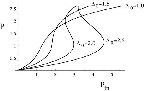
FIG. 1.: The bistability curve is represented for several values of detuning. The chosen pump waist is $w_{p}=2$.

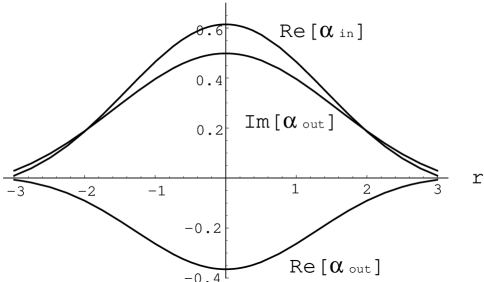
FIG. 2.: The real and imaginary part of the input and ouput stationary fields are represented as a function of $r=(x^{2}+y^{2})^{1/2}$ for $w_{p}=2$, $P_{\rm in}=2.89$, $P=1.06$, $\Delta_{0}=2$.

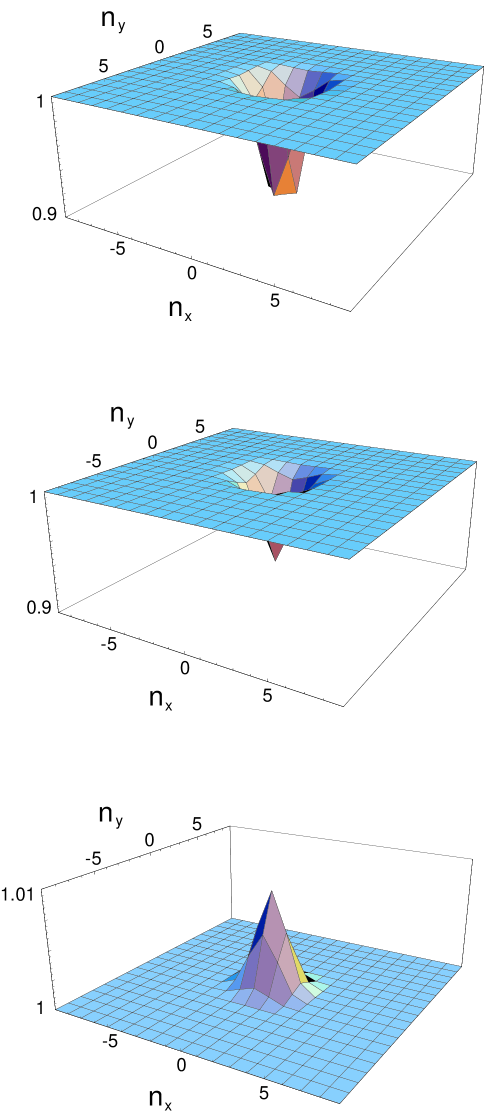
FIG. 3.: The spectrum $S_{{n},{n}}^{\rm out}(\Omega=0.1)$ is plotted vs ${\bf n}$ for several values of $N_{T}$ (from top to bottom $N_{T}=10^{4}$, $10^{5}$, $10^{6}$). Values of other parameters are: $w_{p}=2$, $P_{\rm in}=2.89$, $P=1.06$, $\Delta_{0}=2$, mechanical quality factor $\omega_{m}/\gamma_{m}=10^{6}$.

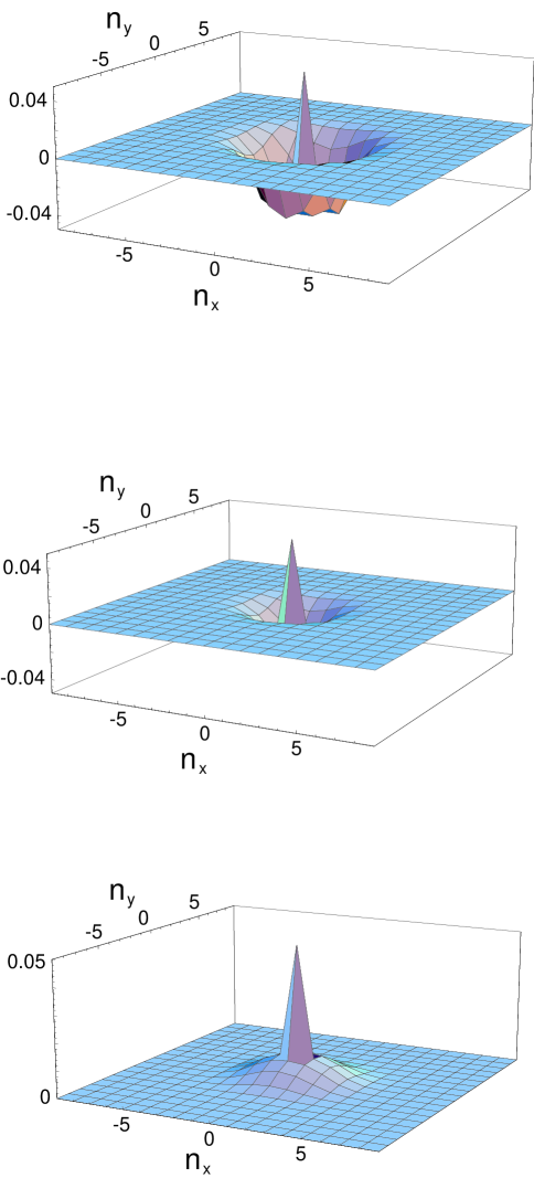
FIG. 4.: The spectrum $S_{{0},{n}}^{\rm out}(\Omega=0.1)$ is plotted vs ${\bf n}$ for several values of $N_{T}$ (from top to bottom $N_{T}=10^{4}$, $10^{5}$, $10^{6}$). Values of other parameters as in Fig.3. In reality, the central peaks of Fig. 4 go out of the actual scale, and their values coincide with those of Fig. 3.

REFERENCES

- [1] L. Hilico, J. M. Courty, C. Fabre, E. Giacobino, I. Abram and J. L. Oudar, Appl. Phys. B 55, 202 (1984).
- [2] P. Meystre, E. M. Wright, J. D. McCallen and E. Vignes, J. Opt. Soc. Am. B 2, 1830 (1985).
- [3] see e.g., A. F. Pace, M. J. Collett and D. F. Walls, Phys. Rev. A 47, 3173 (1994); K. Jacobs, P. Tombesi, M. J. Collett and D. F. Walls, Phys. Rev. A 49, 1961 (1994).
- [4] C. Fabre, M. Pinard, S. Bourzeix, A. Heidmann, E. Giacobino and S. Reynoud, Phys. Rev. A 49, 1337 (1994).
- [5] S. Mancini and P. Tombesi, Phys. Rev. A 49, 4055 (1994); S. Mancini and P. Tombesi, Quantum Semiclass. Opt. 7, 55 (1995).
- [6] S. Mancini, V. I. Man’ko and P. Tombesi, Phys. Rev. A 55, 3042 (1997).
- [7] S. Bose, K. Jacobs and P. Knight, Phys. Rev. A 56, 4175 (1997).
- [8] L. Lugiato, M. Brambilla and A. Gatti, in Advances in Atomic, Mulecular and Optical Physics, 40, 229, B. Bederson and H. Walther eds. (Academic Press, 1998); M. I. Kolobov, Rev. Mod. Phys. 71, 1539 (1999).
- [9] E. Schrödinger, Naturwissenschaften 23, 807, 823, 844 (1935).
- [10] A. Einstein, B. Podolsky and N. Rosen Phys. Rev. 47, 777 (1935).
- [11] W. Unruh, in Quantum Optics, Experimental Gravitation and Measurement Theory, edited by P. Meystre and M. Scully (Plenum, New York, 1983).
- [12] C. W. Gardiner, Quantum Noise, (Springer, Berlin, 1991)
- [13] K. Jacobs, I. Tittonen, H. Wiseman and S. Schiller, Phys. Rev. A 60, 538 (1999); V. Giovannetti and D. Vitali, quant-ph/0006084.
- [14] M. Born and E. Wolf, Principles of Optics, (Pergamon, New York, 1970).
- [15] M. Pinard, Y. Hadjar and A. Heidmann, Eur. Phys. J. D 7, 107 (1999).
- [16] C. W. Gardiner and M. J. Collett, Phys. Rev. A 31, 3761 (1985).
- [17] Y. Hadjar, et al., Europhys. Lett. 46, 545 (1999); I. Tittonen, et al., Phys. Rev. A 59, 1038 (1999).
- [18] V. Giovannetti, S. Mancini and P. Tombesi, quant-ph/0005066.
- [19] see e.g., A. Abramovici, et al, Science 256, 325 (1992).