Positive P simulations of spin squeezing in a two-component Bose condensate

Abstract

The collisional interaction in a Bose condensate represents a non-linearity which in analogy with non-linear optics gives rise to unique quantum features. In this paper we apply a Monte Carlo method based on the positive P pseudo-probability distribution from quantum optics to analyze the efficiency of spin squeezing by collisions in a two-component condensate. The squeezing can be controlled by choosing appropiate collision parameters or by manipulating the motional states of the two components.

I Introduction

In quantum optics it was realized some time ago that so-called ’non-classical’ states of light, in particular, the so-called squeezed states, may outperform classical field states in high precision experiments fabre92:_quant_noise_reduc_optic_system . Moderately squeezed light has been produced, and several non-classical properties have been demonstrated, but classical technology has so far left enough space for improvements that a real practical high precision application of squeezed light remains to be seen. Atomic squeezing is defined in a way similar to squeezing of light, in the sense that the quantum mechanical uncertainty of a physical variable, here a component of the collective spin, is reduced by a suitable manipulation of the quantum state of the system.
Due to quite strong interactions between atoms and between atoms and light, and due to the long storage and interaction times for atoms, the degree of correlations and squeezing obtainable in atomic systems exceeds the one in light by orders of magnitude. Also, there is a real potential for practical application of squeezed atoms, since current atom interferometers and atomic clocks operate at a limit of precision which can only be improved by imposing quantum correlations between the atoms.
Recently there has been a number of proposals for practical spin squeezing: absorption of squeezed light kuzmich97 , quantum non-demolition atomic detection molmer99 , collisional interactions in classical or degenerate gasses pu00 ; sorensen01:_many_bose , photo-dissociation of molecular condensates poulsen01:_quant_states_bose_einst , and controlled dynamics in quantum computers with ions or atoms molmersorensen . Since quantum mechanical squeezing implies quantum mechanical uncertainties below the level in ’natural’ states of the system, e.g., the ground state of the systems, the analysis of squeezing has to be very precise, and in particular one should avoid use of classical approximations or assumptions. In the present paper we shall investigate the possibilities for squeezing in a Bose-Einstein condensate, using a method which takes the interactions and the multi-mode character of the problem exactly into account. We confirm the validity of results of a recent study sorensen01:_many_bose , and we propose an alternative scheme for spin squeezing which relies on a spatial separation of atoms in different internal states.

We consider in this paper a Bose-Einstein condensate of two-level atoms in a trap. The dynamics of such a system is in the second quantized formalism with creation and annihilation operators of atoms in the state $i=a$ or $b$, $\hat{\psi}_{i}^{\dagger}$ , $\hat{\psi}_{i}$ , controlled by the Hamiltonian:

$$\hat{H}=\\ \int\!d^{3}r\Bigl{\{}\sum_{i=a,b}\left[\hat{\psi}^{\dagger}_{i}(\vec{r})\hat{h}_{i}\hat{\psi}(\vec{r})+\frac{g_{ii}}{2}\hat{\psi}^{\dagger}_{i}(\vec{r})\hat{\psi}^{\dagger}_{i}(\vec{r})\hat{\psi}_{i}(\vec{r})\hat{\psi}_{i}(\vec{r})\right]\\ +g_{ab}\hat{\psi}^{\dagger}_{a}(\vec{r})\hat{\psi}^{\dagger}_{b}(\vec{r})\hat{\psi}_{b}(\vec{r})\hat{\psi}_{a}(\vec{r})\Bigl{\}}.$$ (1)

Here, $h_{i}$ is the single particle Hamiltonian for atoms in internal state $i$ and $g_{ij}$ is the effective two-body interaction strength between an atom in state $i$ and one in state $j$. In terms of the corresponding scattering lengths they are given by $g_{ij}=4\pi\hbar^{2}a_{ij}/m$.

At temperatures sufficiently below the critical temperature for Bose-Einstein condensation almost all atoms occupy the same single particle wavefunction which to a very good approximation can be obtained from a two-component Gross-Pitaevskii Equation. There are, however, important effects about which the Gross-Pitaevskii Equation gives no information: the population statistics of the condensate is assumed to be poissonian (or a number state castin98:_low_bose_einst ), it is not treated as a variable which has to be determined, and which can be manipulated by physical processes. In multi-component condensates, the relative populations and coherences of different states are important degrees of freedom which require a more elaborate treatment.

II Two-mode model

In a first attempt to model the population statistics it is convenient for simplicity to assume a separation of the spatial and internal degrees of freedom

$$\hat{\psi}_{a}(\vec{r})=\hat{a}\phi_{a}(\vec{r})\qquad\hat{\psi}_{b}(\vec{r})=\hat{b}\phi_{b}(\vec{r}).$$ (2)

The separation (2) is difficult to justify in general but it is certainly reasonable in the initial state that we have in mind: A very pure (T=0) single component condensate is prepared. We then apply a $\pi/2$-pulse, coherently transfering all atoms to an equal superposition of $a$ and $b$. Then Eq.(2) is fulfilled to a good approximation with $\phi_{a}=\phi_{b}$.

In the subsequent dynamics, the wavefunctions $\phi_{a}(x)$ and $\phi_{b}(x)$ may evolve with time, and we describe this evolution with Gross-Pitaevskii Equations

$$i\hbar\partial_{t}\phi_{i}=\left(\hat{h}_{i}+g_{ii}\frac{N}{2}\left|\phi_{i}\right|^{2}+g_{i\underline{i}}\frac{N}{2}\left|\phi_{\underline{i}}\right|^{2}\right)\phi_{i}$$ (3)

where $\underline{a}\equiv b$ and vice versa.

The dynamics associated with distribution of atoms among the two modes is now studied by rewriting Eq.(1) in terms of the $\hat{a}$ and $\hat{b}$ operators:

$$\hat{H}_{\text{two-mode}}=g_{bb}\left(\hat{b}^{\dagger}\hat{b}^{\dagger}\hat{b}\hat{b}-\frac{N}{2}\hat{b}^{\dagger}\hat{b}\right)\int dr^{3}\left|\phi_{b}\right|^{4}\\ +g_{aa}\left(\hat{a}^{\dagger}\hat{a}^{\dagger}\hat{a}\hat{a}-\frac{N}{2}\hat{a}^{\dagger}\hat{a}\right)\int dr^{3}\left|\phi_{a}\right|^{4}\\ +g_{ab}\left(\hat{b}^{\dagger}\hat{a}^{\dagger}\hat{a}\hat{b}-\frac{N}{2}\hat{b}^{\dagger}\hat{b}-\frac{N}{2}\hat{a}^{\dagger}\hat{a}\right)\int dr^{3}\left|\phi_{b}\right|^{2}\left|\phi_{a}\right|^{2}.$$ (4)

All terms in this Hamiltonian commute with $\hat{a}^{\dagger}\hat{a}$ and $\hat{b}^{\dagger}\hat{b}$ and so the interesting dynamics takes place in the coherences between the two internal states. To study these coherences it is convenient to define effective internal spin operators

$$\hat{S}_{+}\equiv\hat{b}^{\dagger}\hat{a}\quad\hat{S}_{-}\equiv\hat{a}^{\dagger}\hat{b}\quad\hat{S}_{z}\equiv\frac{1}{2}\left(\hat{b}^{\dagger}\hat{b}-\hat{a}^{\dagger}\hat{a}\right).$$ (5)

$\hat{S}_{z}$ represents the difference of total population of states $a$ and $b$, a quantity which can be measured, e.g., by laser induced fluoresence in an experiment. $\hat{S}_{+}$ and $\hat{S}_{-}$ or, equivalently, $\hat{S}_{x}\equiv(\hat{S}_{+}+\hat{S}_{-})/2$ and $\hat{S}_{y}\equiv(\hat{S}_{+}-\hat{S}_{-})/2i$ represent the coherences between $a$ and $b$. By suitable couplings they can also be turned into population differences and are therefore interesting observables of the system. In fact it turns out that the quantity that determines the accuracy of a given spectroscopic experiment is the ratio of the measured spin-component (the signal) to the fluctuations in a component perpendicular to it (the noise) wineland94:_squeez . For the initial state prepared by a $\pi/2$ pulse we have $N$ independent atoms all in the same equal superposition of $a$ and $b$. Then the mean spin is in the $xy$-plane and by definition we can take it to be along the $x$-axis. The maximal signal we can obtain is the length of the spin $S=N/2$ and the perpendicular fluctuations are then $S/2$. To improve this “standard quantum limit” signal/noise ratio we can introduce correlations among the atoms i.e. we can introduce spin squeezing.

With the internal spin operators of Eq. (5) the Hamiltonian (4) can be written

$$\hat{H}_{\text{two-mode}}=e(t)\hat{N}+k(t)\hat{S}_{z}\\ +E(t)\hat{N}^{2}+D(t)\hat{N}\hat{S}_{z}+\chi(t)\hat{S}_{z}^{2}$$ (6)

where the time dependent coefficients are given by integrals involving the time dependent mode functions found from Eq.(3). All the terms in the Hamiltonian (6) commute which is an important simplification as the coefficients are time-dependent. The term proportional to $\hat{S}_{z}$ will result in a rotation of the spin around the $z$-axis. The $\hat{N}$ and $\hat{N}^{2}$ terms give different dynamical overall phases to states with different total numbers of atoms. Such phases are immaterial if we have no external phase-standard to compare with and we neglect these terms for the purpose of the present work. The $\hat{N}\hat{S}_{z}$-term adds to the spin rotation with an angle linear in $N$. It cannot be neglected as the direction of the spin (the phase between $a$- and $b$-components) can be probed by a second $\pi/2$ pulse phase locked to the first $\pi/2$ pulse. The term of interest to us is $\hat{S}_{z}^{2}$, the effect of which is well known from the work of Kitagawa and Ueda kitagawa93:_squeez . It produces spin-squeezing, i.e. it entangles the individual atoms in a way that reduces the fluctuations of the total spin in one of the directions perpendicular to the average spin. The strength parameter of the squeezing operator is given by

$$\chi(t)=\int\!dr^{3}\;\frac{1}{2}\left(g_{bb}\left|\phi_{b}\right|^{4}+g_{aa}\left|\phi_{a}\right|^{4}-2g_{ab}\left|\phi_{a}\right|^{2}\left|\phi_{b}\right|^{2}\right).$$ (7)

Given the time integral $\mu=2\int\!\chi(t^{\prime})dt^{\prime}$ of this parameter Kitagawa and Ueda provide the analytical expressions for the variance of the squeezed spin component

$$\langle\Delta S_{\theta}^{2}\rangle=\\ \frac{S}{2}\left\{[1+\frac{1}{2}(S-\frac{1}{2})A]-\frac{1}{2}(S-\frac{1}{2})\sqrt{A^{2}+B^{2}}]\right\}$$ (8)

where $A=1-\cos^{2S-1}\mu$ and $B=4\sin\mu/2\cos^{2S-2}\mu/2$, and they specify the direction of the squeezed spin component $\hat{S}_{\theta}=\cos\theta\hat{S}_{y}+\sin\theta\hat{S}_{z}$:

$$\theta=\frac{\pi}{2}+\frac{1}{2}\arctan\frac{B}{A}.$$ (9)

It is of some interest to use simple analytical approximations for $\chi(t)$ and we will do so in the specific cases studied below. Another approach would of course be to obtain $\chi(t)$ by a numerical solution of Eq. (3).

III Full multi-mode description

Equations (2)-(7) are based on a simplifying assumption. The actual observables of the system are more complicated to deal with, but we can define a set of operators obeying angular momentum commutation relations by

$$\hat{J}_{x} \equiv\frac{1}{2}\int dr^{3}\left(\hat{\psi}_{b}^{\dagger}\hat{\psi}_{a}+\hat{\psi}_{a}^{\dagger}\hat{\psi}_{b}\right)$$ (10)

$$\hat{J}_{y} \equiv\frac{1}{2i}\int dr^{3}\left(\hat{\psi}_{b}^{\dagger}\hat{\psi}_{a}-\hat{\psi}_{a}^{\dagger}\hat{\psi}_{b}\right)$$ (11)

$$\hat{J}_{z} \equiv\frac{1}{2}\int dr^{3}\left(\hat{\psi}_{b}^{\dagger}\hat{\psi}_{b}-\hat{\psi}_{a}^{\dagger}\hat{\psi}_{a}\right).$$ (12)

The total number operator $\hat{N}\equiv\int dr^{3}(\hat{\psi}_{a}^{\dagger}\hat{\psi}_{a}+\hat{\psi}_{b}^{\dagger}\hat{\psi}_{b})$ commutes with these three operators and when the two-mode approximation applies well, the two-mode and multi-mode operators are comparable by the replacement

$$\hat{J}_{+}=\rho e^{i\nu}\hat{S}_{+}\quad\hat{J}_{-}=\rho e^{-i\nu}\hat{S}_{-}\quad\hat{J}_{z}=\hat{S}_{z}$$ (13)

where $\rho e^{i\nu}\equiv\int dr^{3}\phi_{b}^{*}(\vec{r})\phi_{a}(\vec{r})$. The factor $\rho$ takes into account that $\langle\hat{J}_{x}\rangle$ and $\langle\hat{J}_{y}\rangle$ vanish unless the atoms in state $a$ and $b$ occupy the same region in phase space and $\nu$ is a dynamical phase from the spatial dynamics.

The two-mode approximation provides an intuitive picture of the evolution of the system. It is however not easy to justify the factorization (2) and we shall therefore apply an exact method to determine more precisely what happens to the mean values and the variances of the components of $\hat{\vec{J}}$. The positive P function ($P_{+}$) gardiner91:_quant_noise is a pseudo-probability distribution giving expectation values of normally ordered operator products as c-number averages. In our case with two internal states one has

$$\langle:\!f[\hat{\boldsymbol{\psi}}(t)]\!:\rangle=\int\!d[\boldsymbol{\psi}]f[\boldsymbol{\psi}]P_{+}[\boldsymbol{\psi},t]$$ (14)

where

$$\hat{\boldsymbol{\psi}}(t)\equiv\left(\begin{array}[]{c}\hat{\psi}_{a}(t)\\ \hat{\psi}_{a}^{\dagger}(t)\\ \hat{\psi}_{b}(t)\\ \hat{\psi}_{b}^{\dagger}(t)\end{array}\right)\quad\text{and}\quad\boldsymbol{\psi}\equiv\left(\begin{array}[]{c}\psi_{a1}\\ \psi_{a2}\\ \psi_{b1}\\ \psi_{b2}\end{array}\right).$$ (15)

The distribution is not determined uniquely but one particular choice obeys a functional Fokker-Planck equation which is of course immensely difficult to solve. For numerical purposes it is much better to translate it to coupled Langevin equations for the 4 c-number fields (“wave functions”). These equations are “noisy Gross-Pitaevskii equations”

$$d\psi_{i\mu}=(-1)^{\mu}\frac{idt}{\hbar}\left(\hat{h}_{i}+g_{ii}\psi_{i2}\psi_{i1}+g_{ab}\psi_{\underline{i}2}\psi_{\underline{i}1}\right)\psi_{i\mu}+dW_{i\mu}$$ (16)

where $\underline{a}\equiv b$ and vice versa. In order to treat the interactions exactly (within the approximation given by the form of Eq.(1)) the noise terms have to be gaussian and to fulfill:

$$\langle dW_{i\mu}(\vec{r},t)\rangle=0$$ (17)

$$\begin{split}\langle dW_{i\mu}(\vec{r},t)dW_{j\nu}&(\vec{r}^{\prime},t^{\prime})\rangle=\delta^{(3)}(\vec{r}\!-\!\vec{r}^{\prime})\delta(t\!-\!t^{\prime})\delta_{\mu\nu}\\ &\times(-1)^{\mu}\frac{idtg_{ij}}{\hbar}\psi_{i\mu}(\vec{r},t)\psi_{j_{\mu}}(\vec{r},t).\end{split}$$ (18)

On the computer we can simulate the Langevin equations to obtain an ensemble of realizations of $\boldsymbol{\psi}$. This ensemble is a finite sampling of $P_{+}$ and can therefore be used to calculate expectation values via the prescription (14) and with a precision limited only by the number of realizations in the ensemble.

Three limitations of the method should be noted: (i) The initial state of the system has to be expressed as an initial $P_{+}$. This is trivial for a single coherent state and for any mixture of coherent states but it can be complicated for other initial conditions. (ii) The $P_{+}$ method has a notorious divergence problem at large non-linearities. This problem sets in after a certain time and is clearly noticable in the simulations. We can therefore easily tell how long we can trust the results of the method. (iii) Although we have so far written all equations in 3D it would be computationally very heavy to simulate a sufficient number of realizations of Eq. (16). In what follows we will thus restrict ourselves to 1D. It is reasonable to assume that this may alter the quantitative results significantly but a 1D calculation can be used to investigate the validity of the two-mode model which may hereafter be applied in 3D with more confidence.

IV Spin squeezing with controlled collision strengths

Let us first focus on a situation with simple spatial dynamics. If we set $V_{a}=V_{b}=m\omega^{2}x^{2}/2$ (1D model) and we assume that the values of the collision strengths can be controlled so that, e.g., $g_{aa}=g_{bb}=2g_{ab}\equiv g$ the spatial dynamics is limited to a slight breathing. The spin-dynamics is almost a pure squeezing, that is, the mean spin stays in the $x$-direction. To get an estimate of the strength parameter $\chi$ of Eq. (7) we find $\phi_{a}(t=0)=\phi_{b}(t=0)$ as the Thomas-Fermi approximation to the stationary solution of the GPE with all atoms in the $a$-state. We then have:

$$\chi\cong\frac{1}{2^{2/3}3^{2/3}5}\frac{g^{2/3}}{N^{1/3}}m^{1/3}\omega^{2/3}.$$ (19)

Choosing $g=0.005\hbar\omega a_{0}$ and $N=2000$ we get $\chi=6.1\times 10^{-4}\hbar\omega$ which should give a sizable squeezing within a quarter of a trapping periode. $a_{0}\equiv\sqrt{\frac{\hbar}{m\omega}}$ is the harmonic oscillator length in the trap and $m$ is the atomic mass.

In Fig.1

Figure 1: Squeezing of the collective spin for favorable interaction parameters: N=2000 atoms and $(g_{aa},g_{ab},g_{bb})=(1.0,0.5,1.0)\times 5\times 10^{-3}\hbar\omega a_{0}$ (1D model). $+$ (with errorbars) show $P_{+}$ results, lines show results of the two-mode model.

we show results of both the two-mode approximation (8) and of the $P_{+}$ simulation for the parameters mentioned above. $\chi$ was assumed to be constant and of the value determined by Eq. (19). $\hat{J}_{\theta}=\cos\theta\hat{J}_{y}+\sin\theta\hat{J}_{z}$ refers to the squeezed component of the spin. The direction $\theta$ in the $yz$-plane is determined in the two mode model, i.e., from Eq. (9) and it is not independently optimized for the full $P_{+}$ results. The agreement is seen to be surprisingly good considering the crudeness of the estimate of the parameters in the two mode model. Within the uncertainty of the positive P results (the $\langle\Delta\hat{J}_{\theta}^{2}\rangle$ data are presented with errorbars in Fig. 1) the noise suppression is seen to be almost perfect. These calculations thus confirm the results of Sørensen et al. sorensen01:_many_bose where the simple two-mode approach was supplemented by another approximate method.

V Spin squeezing with controlled mode functions overlaps

In the experiments on the $|F=1,m_{f}=-1\rangle$ and $|F=2,m_{f}=1\rangle$ states in ⁸⁷Rb hall98:_dynam_compo_sepa the scattering lengths and thus the interaction strengths are actually in proportion $g_{aa}:g_{ab}:g_{bb}=1.03:1:0.97$. This is far from ideal conditions for squeezing as we can see from Eq. (7): $\chi=0$ when in addition $\phi_{a}=\phi_{b}$ as is the case initially. To produce a sizable squeezing effect we propose to make the two mode functions differ (see also goldstein00:_elimin_mean_field_shift_two ). This is achieved by applying different potentials to the two internal states which has actually already been done for magnetically trapped Rb making use of gravity and different magnetic moments of the two internal states hall98:_dynam_compo_sepa . If $V_{b}$ is displaced from $V_{a}$ the $b$-component created by the initial $\pi/2$-pulse will move away from the $a$ component thereby reducing the overlap $\int\!dx\left|\phi_{a}\right|^{2}\left|\phi_{b}\right|^{2}$ and increasing $\chi$. It is remarkable that the squeezing then takes place while the two components are away from each other and are therefore not interacting.

To demonstrate the accomplishments of the scheme described above we have chosen simply to displace $V_{b}$ by a certain amount $x_{0}$ from $V_{a}$. In this model both potentials are still harmonic and of the same strength. The spatial dynamics is now more complicated but it can be approximated by the solutions to coupled Gross-Pitaevskii equations. To get a rough idea of the evolution we can use the well know evolution of a displaced ground state wavefunction in a harmonic trap. We then get

$$\rho e^{i\nu}=e^{-x_{0}^{2}\left(1-\cos(\omega t)\right)/2}e^{ix_{0}^{2}\sin(\omega t)/2}$$ (20)

and

$$\int\left|\phi_{b}\right|^{2}\left|\phi_{a}\right|^{2}dx=\frac{1}{\sqrt{2\pi}}\;e^{-x_{0}^{2}\left(1-\cos(\omega t)\right)/4}.$$ (21)

If we choose $(g_{aa},g_{ab},g_{bb})=(1.03,1,0.97)\times 5\times 10^{-3}\hbar\omega a_{0}$ and $x_{0}=3a_{0}$ this model gives an order of magnitude estimate for the integrated strength parameter of $\int_{0}^{2\pi/\omega}\chi(t)dt\cong 10^{-2}\hbar\omega$ when the two components are again overlapped. For 2000 atoms this corresponds to a reduction of the uncertainty in the squeezed spin component by roughly a factor of 10 according to Eq. 8.

In Fig.2

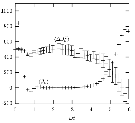
Figure 2: Squeezing due to spatial separation of the two internal state potentials by $x_{0}=3a_{0}$. The total number of atoms is 2000 and the interaction strengths are $(g_{aa},g_{ab},g_{bb})=(1.03,1,0.97)\times 5\times 10^{-3}\hbar\omega a_{0}$ (1D model).

we use these estimates to analyze the $P_{+}$ simulations, i.e., we plot the expectation value of the spin component predicted to be maximal, $\langle\hat{J}_{\nu}\rangle$ , and the variance of the perpendicular component predicted to be squeezed, $\langle\Delta\hat{J}_{\theta}^{2}\rangle$. As can be seen, after a fast drop a large fraction of the original mean spin is recovered in $\langle\hat{J}_{\nu}\rangle$ when the two wave packets are again overlapped. This confirms our prediction of $\nu$ and it implies that a sizable signal can be obtained in an experiment. At the same time the variance in the predicted perpendicular component is strongly suppressed confirming our prediction for $\theta$ and implying that the noise in the experiment can be significantly reduced below the standard quantum limit.

VI Discussion

We have presented the first exact numerical studies of spin squeezing in two-component condensates. As in our previous work on squezing of a single component atomic field operator poulsen01:_quant_states_bose_einst we have applied the positive P distribution which is well suited for studies of transient, short time behavior of interacting many-body systems. This formulation involves simulations, and due to the formal separation of c-number representations of creation and annihilation operators, ’non-physical’ results may occur such as negative/complex atomic densities, and few instants with negative variances as depicted in Figs. 1 and 2. For long times we cannot exclude that slight imprecision due to discretization of space and time contributes to these results. The Monte Carlo nature of the method makes it somewhat tedious to check rigorously for discretization errors but for resonable numbers of realizations in the ensemble sampling errors will dominate anyhow.

The conclusion of this paper is that the predictions of the simple two-mode model reproduce the full multimode result also quantitatively. This means that the spatio-temporal dynamics and the population dynamics couple the way they should to produce spin squeezing but the resulting entanglement between spatial and internal degrees of freedom is small enough that purely internal state observables show strong squeezing and multi-particle entanglement. In particular the calculations of Fig. 2 reveal that quite significant distortions of the distributions when the components separate and merge do not prevent sizable spin squeezing.

Although we claim quantitative agreement above it should of course be realized that this is within the 1D model. To use the two-mode model to describe a real experiment the spatial dynamics which enters the internal dynamics via Eqs. (7) and (13) must be treated with some accuracy. Apart from the 3D aspects it should be noted that e.g. in some experiments on two-component condensates myatt97:_produc_overlap the displacement of the potentials are accompanied (and in fact due to) different strenghts of the potentials. This adds to the complexity of the dynamics and will of course be important if the aim is precise quantitative predictions and not a proof-of-principle analysis as offered in this paper.

More tests need to be carried out for other kinds of processes, but the present study suggests that the simple two-mode description provides good predictions for the many-body dynamics of spin squeezing. Hence other ideas, e.g., for reducing the fluctuations in the total number of atoms in a condensate or in out-coupled atom laser beams, may be reliably based on the terms of Eq. (6).

References

- (1) C. Fabre and E. Giacobino (eds.), Quantum Noise Reduction in Optical Systems, Special issue of Appl. Phys. B 55, (1992).
- (2) A. Kuzmich et al, Phys. Rev. Lett. 79, 4782 (1997); J. Hald et al, Phys. Rev. Lett. 83, 1319 (1999); A. E. Kozhekin et al, Phys. Rev. A 62 033809 (2000).
- (3) K. Mølmer, Eur. Phys. J. D 5, 301 (1999); A. Kuzmich et al, Europhys. Lett. 42, 481 (1998); A. Kuzmich et al Phys. Rev. Lett. 85, 1594 (2000).
- (4) H. Pu and P. Meystre, Phys. Rev. Lett. 85, 3987 (2000); L.-M. Duan et al, ibid 3991;
- (5) A. Sørensen, L.-M. Duan, I. Cirac, and P. Zoller, Nature 409, 63 (2001).
- (6) U. V. Poulsen and K. Mølmer, Phys. Rev. A. 63, 023604 (2001).
- (7) K. Mølmer and A. Sørensen, Phys. Rev. Lett. 82, 1835 (1999); A. Sørensen and K. Mølmer, Phys. Rev. Lett. 83, 2274 (1999).
- (8) Y. Castin and R. Dum, Phys. Rev. A 57, 3008 (1998).
- (9) D. J. Wineland, J. J. Bollinger, and W. M. Itano, Phys. Rev. A 50, 67 (1994).
- (10) M. Kitagawa and M. Ueda, Phys. Rev. A 47, 5138 (1993).
- (11) C. W. Gardiner, Quantum Noise (Springer-Verlag, Berlin Heidelberg, 1991).
- (12) D. S. Hall et al, Phys. Rev. Lett. 81, 1539 (1998).
- (13) E. V. Goldstein, M. G. Moore, H. Pu, and p. Meystre, Phys. Rev. Lett. 85, 5030 (2000).
- (14) C. J. Myatt et al, Phys. Rev. Lett. 78, 586 (1997).