Violations of local realism with quNits up to $N=16$.

Abstract: Predictions for systems in entangled states cannot be described in local realistic terms. However, after admixing some noise such a description is possible. We show that for two qu$N$its (quantum systems described by $N$ dimensional Hilbert spaces) in a maximally entangled state the minimal admixture of noise increases monotonically with $N$. The results are a direct extension of those of Kaszlikowski et. al., Phys. Rev. Lett. 85, 4418 (2000), where results for $N\leq 9$ were presented. The extension up to $N=16$ is possible when one defines for each $N$ a specially chosen set of observables. We also present results concerning the critical detectors efficiency beyond which a valid test of local realism for entangled qu$N$its is possible.

In early 1990’s Peres and Gisin [1] have shown, that if one considers certain dichotomic observables applied to maximally entangled state of two qu$N$its (particles described by an $N$-dimensional Hilbert space), the violation of local realism, or more precisely of the CHSH inequalities, survives the limit of $N\rightarrow\infty$ and is maximal there. However, for any dichotomic quantum observables the CHSH inequalities give violations bounded by the Tsirelson limit [2], i.e., it is limited by the factor of $\sqrt{2}$. Therefore, the question whether the violation of local realism increases with growing $N$ was still left open.

It has been recently shown [3] that one indeed observes an increase with $N$ of the discrepancy between quantum and local realistic description of two maximally entangled qu$N$its observed via unbiased multiport beamsplitters [4]. The results presented in [3] have been obtained via a numerical method of linear optimisation and have been limited to $N=9$ [5].

In the present paper we extend the computations up to $N=16$. In the case of the method presented in [3] for $N\geq 10$ the computational time was prohibitively long. We avoid this problem here by a careful choice of a fixed set of two pairs of observables for each $N$. As a result one can avoid the time consuming search for optimal sets of observables, which was a part of the computer program used in [3].

Another critical parameter for any Bell-type test is the threshold efficiency of the detector to make it an unconditionally valid test of local realism. The efficiency a detector is usually defined as its probability to fire when the quantum particle enters it. The procedure used in [3] can be easily adapted to handle also the question of inefficient detectors. We report here the threshold values of efficiency for $N$ up to $16$. It decreases with $N$, however the decrease is very slow.

Let us consider two qu$N$it systems described by the mixed states in the form

$$\rho_{N}(F_{N})=F_{N}\rho_{noise}+(1-F_{N})|\Psi_{max}^{N}\rangle\langle\Psi_{max}^{N}|,$$ (1)

where $|\Psi_{max}^{N}\rangle$ is a maximally entangled two qu$N$it state, $\rho_{noise}=\frac{1}{N^{2}}\hat{I}$, and the positive parameter $F_{N}\leq 1$ determines the “noise fraction” within the full state. The threshold minimal $F_{N}^{tr}$, for which the state $\rho_{N}(F_{N})$ allows a local realistic model, will be our numerical value of the strength of violation of local realism by the quantum state $|\Psi_{max}\rangle$. The higher is $F_{N}^{tr}$ the higher is the minimum noise admixture required to hide the nonclassicality of the quantum prediction.

To overcome the mentioned Tsirelson limit one has to use non-dichotomic observables. Here, as in the previous work, we limit ourselves to observables defined by unbiased multiport beamsplitters.

Unbiased $2N$-port beamsplitters [7] are devices with the following property: if one photon enters into any single input port (out of the $N$), its chances of exit are equally split between all $N$ output ports. The unbiased multiports are an operational realization of the concept of mutually unbiased bases, see [8]. Such bases are ”as different as possible” [9], i.e. fully complementary. The 50-50 beamsplitter is the simplest member of the family.

One can always build an unbiased multiport with the distinguishing trait that the elements of its unitary transition matrix, ${\bf U}^{N}$, are solely powers of the $N$-th root of unity $\gamma_{N}=exp{(i2\pi/N)},$ namely ${\bf U}^{N}_{ji}=\frac{1}{\sqrt{N}}\gamma_{N}^{(j-1)(i-1)}.$ Devices endowed with such a matrix were proposed to be called Bell multiports [10].

Let us now imagine spatially separated Alice and Bob who perform the experiment of (1). The maximally entangled state of the two qu$N$its

$$\mid\Psi^{N}_{max}\rangle={1\over\sqrt{N}}\sum^{N}_{m=1}\mid m,A\rangle\mid m,B\rangle,$$ (2)

where e.g. $\mid m,A\rangle$ describes a photon in mode $m$ propagating to Alice, can be prepared with the aid of parametric down conversion (see [10]). The two sets of $N$ phase shifters at the inputs of the multiports, which are denoted as $N$ dimensional ”vectors of phases” $\vec{\phi}_{A}=(\phi^{1}_{A},\phi^{2}_{A},\dots,\phi^{N}_{A})$ for Alice and $\vec{\phi}_{B}=(\phi^{1}_{B},\phi^{2}_{B},\dots,\phi^{N}_{B})$ for Bob, introduce phase factor $e^{i(\phi^{m}_{A}+\phi^{m}_{B})}$ in front of the $m$-th component of the initial state (2), where $\phi^{m}_{A}$ and $\phi^{m}_{B}$ denote the local phase shifts. Alice measures two observables $A_{1},A_{2}$ defined by sets of phase shifts $\vec{\phi}_{A_{1}},\vec{\phi}_{A_{2}}$ whereas Bob measures two observables $B_{1},B_{2}$ defined by sets of the phase shifts $\vec{\phi}_{B_{1}},\vec{\phi}_{B_{2}}$.

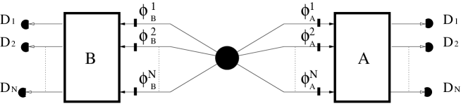
FIG. 1.: The experiment of Alice and Bob with entangled qu$N$its. Each of their measuring apparata consist of a set of $N$ phase shifters (PS) just in front of an $2N$ port Bell multiport, and $N$ photon detectors $D_{k},D_{l}$ (perfect, in the gedanken situation described here) which register photons in the output ports of the device. The phase shifters serve the role of the devices which set the free macroscopic, classical parameters which can be controlled by the experimenters. The source produces a beam entangled two particle state.

Each set of local phase shifts constitutes the interferometric realizations of the ”knobs” at the disposal of the observer controlling the local measuring apparatus which incorporates also the Bell multiport and $N$ detectors. In this way the local observable is defined. Its eigenvalues refer simply to registration at one of the $N$ detectors behind the multiport. The quantum prediction for the joint probability $P^{QM}_{F_{N}}(k,l)$ to detect a photon at the $k$-th output of the multiport A and another one at the $l$-th output of the multiport B calculated for the state (1) is given by:

$$P^{QM}_{F_{N}}{(k,l;\phi^{1}_{A},...\phi^{N}_{A},\phi^{1}_{B},...\phi^{N}_{B})}={1-F_{N}\over N}\left|\sum^{N}_{m=1}\exp{[i(\phi^{m}_{A}+\phi^{m}_{B})]}{\bf U}^{N}_{mk}{\bf U}^{N}_{ml}\right|^{2}+{F_{N}\over N^{2}}$$ (3)

$$={1-F_{N}\over N^{3}}\left(N+2\sum^{N}_{m>n}\cos{({\bf\Phi}^{m}_{kl}-{\bf\Phi}^{n}_{kl})}\right)+{F_{N}\over N^{2}},$$ (4)

where ${\bf\Phi}^{m}_{kl}\equiv\phi^{m}_{A}+\phi^{m}_{B}+[m(k+l-2)]\frac{2\pi}{N}$. The counts at a single detector, of course, do not depend upon the local phase settings: $P^{QM}_{F_{N}}{(k)}=P^{QM}{(l)}_{F_{N}}={1}/{N}.$

The essential result of [3] is that qu$N$its violate local realism more strongly than qubits in the following sense: the required minimal admixture of pure noise to the maximally entangled state, such that a local realistic description of the quantum predictions becomes possible, increases with $N$. This result has been obtained via numerical methods of linear optimisation. Here we give a brief account of the method sending the reader for a more detailed description to [3].

It is well known (see, e. g. [11], [14]) that the hypothesis of local hidden variables is equivalent to the existence of a (non-negative) joint probability distribution involving all four observables ($A_{1},A_{2},B_{1},B_{2}$) from which it should be possible to obtain all the quantum predictions as marginals. Let us denote this hypothetical joint distribution by $P^{HV}(k_{1},k_{2},l_{1},l_{2})$, where $k_{1}$ and $k_{2}$ represent the outcome values for Alice’s measurement of observables $A_{1}$ and $A_{2}$, and $l_{1}$ and $l_{2}$ represents the outcome values for Bob’s measurement of observables $B_{1}$ and $B_{2}$. In quantum mechanics one cannot even define such a distribution, since it involves mutually incompatible measurements. A given set of quantum predictions, here $P^{QM}_{F_{N}}(k_{i},l_{j}|A_{i},B_{j})$, is reproducible by $P^{HV}(k_{1},k_{2},l_{1},l_{2})$, if and only if

$$P^{QM}_{F_{N}}(k_{i},l_{j}|A_{i},B_{j})=\sum_{k_{i+1}}\sum_{l_{j+1}}P^{HV}(k_{1},k_{2},l_{1},l_{2}),$$ (5)

where $k_{i+1}$ and $l_{j+1}$ are understood as modulo $2$. The Bell Theorem, within this context, says that there are quantum predictions, which for $F_{N}$ below a certain threshold cannot be modelled by (5), i.e. there exists a critical $F_{N}^{tr}$ below which one cannot have any local realistic model. The $4N^{2}$ linear equations (5) imposed on $N^{4}$ local hidden probabilities $P^{HV}(k_{1},k_{2},l_{1},l_{2})$ form the full set of necessary and sufficient conditions for the existence of local and realistic description of the experiment. This is a typical linear optimisation problem with $N^{4}+1$ non-negative unknowns, $P^{HV}(k_{1},k_{2},l_{1},l_{2})$ and $F_{N}$, and $4N^{2}$ linear conditions (5).

In the previous work [3] an involved computer algorithm [12] was used to

• (i) solve the linear optimization problem for finding a minimal threshold $F_{N}^{tr}$ for which, under specific chosen settings, (5) is satisfied,

• (ii) find such settings for which (i) gives highest possible value $F_{N}^{tr}$ (the so called ”amoeba” procedure was used [13]).

Since the task (ii) makes the computation, for high $N$, highly time consuming (since for each set of settings (i) has to be solved), the results of [3] reach only $N=9$.

Here we avoid this problem by dropping the point (ii) altogether. We search for $F_{N}^{tr}$ for a specific single set of observables $A^{(N)}_{1},A^{(N)}_{2},B^{(N)}_{1},B^{(N)}_{2}$ for each $N$. We have used the phase settings in the following form: $\vec{\phi}_{A_{1}}=(0,0,\dots,0),\vec{\phi}_{A_{2}}=(0,{\pi\over N},{2\pi\over N}\dots,{(N-1)\pi\over N})$ for Alice and $\vec{\phi}_{B_{1}}=(0,{\pi\over 2N},{2\pi\over 2N},\dots,{(N-1)\pi\over 2N}),\vec{\phi}_{B_{2}}=-\vec{\phi}_{B_{1}}$ for Bob. For $N=2$ $\phi_{A_{1}}^{2}=0,\phi_{A_{2}}^{2}={\pi\over 2}$, $\phi_{B_{1}}^{2}={\pi\over 4},\phi_{B_{2}}^{2}=-{\pi\over 4}$. These are the standard phases for the maximal violations of local realism in a two qubit experiment (the first phase in each ”phase vector” is irrelevant). For $N=3$, $\vec{\phi}_{A_{1}}=(0,0,0)$, $\vec{\phi}_{A_{2}}=(0,{\pi\over 3},{2\pi\over 3})$ and $\vec{\phi}_{B_{1}}=(0,{\pi\over 6},{\pi\over 3})$, $\vec{\phi}_{B_{2}}=(0,-{\pi\over 6},-{\pi\over 3})$ give maximal violation of local realism (a result of [3] discussed in [15]). For $N\geq 4$ the phases were guessed. However, for up to $N=9$ these phases have given exactly the same results as that obtained with the second stage of optimisation in [3]. Of course, we do not know if they are really optimal for $N\geq 10$ because there is no data for comparison. Nevertheless, the violation of local realism obtained for these phases still grows with $N$ as it is depicted in FIG2. and the growth has the same character as for $N\leq 9$.

FIG. 2.: Dependence of the critical noise admixture to the maximally entangled state (2) on the dimension of the Hilbert space of a single subsystem. For larger noise then shown here local realistic description exists. The increase of the value is interpreted as an objective measure of the increasing with $N$ non-classicality of pairs of entangled qu$N$its.

Another interesting question that may be raised here concerns the critical quantum efficiency of detectors below which there exists a local and realistic description of the system. It was showed [17] that for $N=2$ the critical efficiency equals $2\sqrt{2}-2(\approx 0.828)$. Taking into account that violation of local realism grows with $N$ one may expect that for higher dimensions of Hilbert space the critical efficiency is lower than for two qubits. This problem has not been investigated in our previous work. Here we show that the presented method can be just as well applied to study this.

To this end it is necessary to modify the conditions (5) so as to take into account the probabilities of non detection events, which are characterised by the quantum efficiency of detectors $\eta$ ($0\leq\eta\leq 1$) (for simplicity we assume that the efficiencies of all detectors are the same). This can be achieved as follows. To a local non-detection event we ascribe the additional value that differs from the values ascribed to the firings of detectors, say $0$. In this case there are more local hidden probabilities and more linear constraints imposed on them for now the indices enumerating possible events extend from $0$ to $N$ (before the range was $1,\dots N$).

For non-ideal detectors, each endowed with identical inefficiency, the quantum probabilities $P^{QM}_{F_{N},\eta}(k_{i},l_{j}|A_{i},B_{j})$ of coincidences between detector $k_{i}$ at Alice’s side and detector $l_{j}$ at Bob’s side ($k_{i},l_{j}\neq 0$) while measuring observables $A_{i},B_{j}$ are equal to the corresponding probabilities with ideal detectors ($\eta=1$) multiplied by $\eta^{2}$, i.e., $P^{QM}_{F_{N},\eta}(k_{i},l_{j}|A_{i},B_{j})=\eta^{2}P^{QM}_{F_{N}}(k_{i},l_{j}|A_{i},B_{j})$. The quantum probabilities $P^{QM}_{F_{N},\eta}(0,l_{j}|A_{i},B_{j})$ and $P^{QM}_{F_{N},\eta}(k_{i},0|A_{i},B_{j})$ ($l_{i}\neq 0,k_{i}\neq 0$) of events when one detector fails to fire at one of the sides of the experiment equals ${1\over N}\eta(1-\eta)$ whereas the probability of the event when both detectors fail to fire $P^{QM}_{F_{N},\eta}(0,0|A_{i},B_{j})$ is $(1-\eta)^{2}$. Replacing left hand sides of (5) by appropriate quantum probabilities, i.e. $P^{HV}(k_{i},l_{j}|A_{i},B_{j})=P^{QM}_{\eta,F_{N}}(k_{i},l_{j}|A_{i},B_{j})$, one again obtains a linear optimisation problem with respect to $F_{N}$, in which there are now $(N+1)^{4}$ local hidden probabilities and $4(N+1)^{2}$ linear constrains.

Due to the fact that $\eta$ enters into equations quadratically it is not possible to optimise it by means of linear programing methods. The simple way of solving this difficulty is the following. One decreases the value of $\eta$ (in our case by one percent) starting from $\eta=1$ and keeping the local phases fixed until the program returns $F_{N}=1$, which signals that for this efficiency there is already a local and realistic description. Of course, the critical efficiency applies only to the case of the observables chosen here. Once different observables or perhaps some non-maximally entangled state (compare [16]) are chosen it may be lower. The results are depicted in FIG3. We see that critical efficiency decreases very slowly but continuously from the value obtained by Garg and Mermin [17] for two qubits ($N=2$).

FIG. 3.: Dependence of critical quantum efficiency of detectors $\eta_{N}^{cr}$ versus the dimension of the Hilbert space $N$.

Acknowledgements

MZ and DK are supported by the University of Gdansk Grant No BW/5400-5-0032-0; DK is supported by Fundacja na Rzecz Nauki Polskiej. TD is affiliated to the Fund for Scientific Research (FWO), Flanders, as a post-doctoral fellow, and member of the research group FUND (V.U.B.). This paper was written in the framework of the Flemish-Polish Scientific Collaboration Program No. 007.

REFERENCES

- [1] A. Peres, Phys. Rev. A 46, 4413 (1992), N. Gisin and A. Peres, Phys. Lett. A 162, 15-17 (1992).
- [2] B. S. Tsirelson, Lett. Math. Phys. 4 93 (1980).
- [3] Dagomir Kaszlikowski, Piotr Gnacinski, Marek Żukowski, Wieslaw Miklaszewski and Anton Zeilinger, Phys. Rev. Lett. 85, 4418 (2000).
- [4] C. Mattle, M. Michler, H. Weinfurter, A. Zeilinger and M. Żukowski, Appl. Phys. B, 60, S111 (1995).
- [5] The number of Bell inequalities grows extremely rapidly together with the increasing dimension of Hilbert space [14], [6] and therefore their direct application becomes prohibitively difficult
- [6] Itamar Pitovsky and Carl Svozil, quant-ph/0011060.
- [7] A. Zeilinger, H.J. Bernstein, D.M. Greenberger, M.A. Horne, and M. Żukowski, in Quantum Control and Measurement, eds. H. Ezawa and Y. Murayama (Elsevier, 1993); A. Zeilinger, M. Żukowski, M.A. Horne, H.J. Bernstein and D.M. Greenberger, in Quantum Interferometry, eds. F. DeMartini, A. Zeilinger, (World Scientific, Singapore, 1994).
- [8] I.D. Ivanovic, J. Phys. A 14, 3241 (1981); W.K. Wooters, Found. Phys. 16, 391 (1986); J. Schwinger, Proc. Nat. Acad. Sc. 46, 570 (1960).
- [9] A.Peres, Quantum theory: Concepts and Methods (Kluwer, Dordrecht, 1993).
- [10] M. Żukowski, A. Zeilinger, and M. A. Horne, Phys. Rev. A 55, 2564 (1997).
- [11] A. Fine, J. Math. Phys. 23, 1306 (1982)
- [12] J. Gondzio, European Journal of Operational Research 85, 221 (1995); J. Gondzio, Computational Optimization and Applications 6, 137 (1996).
- [13] J. A. Nelder and R. Mead, Computer Journal 7, 308-313 (1965).
- [14] A. Peres, Found. Phys. 29, 589 (1999)
- [15] Dagomir Kaszlikowski, quant-ph/0008086.
- [16] P. H. Eberhard, Phys. Rev. A 47, R747 (1993).
- [17] A. Garg, N. D. Mermin, Phys. Rev. Lett. 49, 901 (1982).