Quantum Information Theory – an Invitation

R.F. Werner^‡

Institut für Mathematische Physik, TU Braunschweig

Mendelssohnstr. 3 / 38106 Braunschweig / Germany

October 30, 2000

This text is part of a volume entitled “Quantum information — an introduction to basic theoretical concepts and experiments”, to be published in Springer Tracts in Modern Physics. Authors will be G. Alber, T. Beth, M., P., and R. Horodecki. M. Rötteler, H. Weinfurter, R.F. Werner, and A. Zeilinger. Articles:

G. Alber From the foundations of quantum theory to quantum technology - an introduction R.F. Werner This article H. Weinfurter, A. Zeilinger Quantum communication Th. Beth, M. Rötteler Quantum algorithms: applicable    algebra und quantum physics M., P., and R. Horodecki Mixed-state entanglement    and quantum communication Joint index Joint list of references

References to “articles in this book” will be to these articles.

^‡Email: r.werner@tu-bs.de
Web: http://www.imaph.tu-bs.de/qi

Chapter 1 Introduction

Quantum Information and Quantum Computers have received a lot of public attention recently. Quantum Computers have been advertised as a kind of warp drive for computing, and indeed the promise of the algorithms by Shor and Grover is to perform computations which are extremely hard or even provably impossible on any merely “classical” computer. On the experimental side, perhaps the most remarkable feat of Quantum Information processing was the realization of “quantum teleportation”, which once again has science fiction overtones.

In some sense these miracles are an extension of the Strangeness of Quantum Mechanics – those unresolved questions in the foundations of quantum mechanics, which most physicists know about, but few try to tackle directly in their research. However, trying to build an explanation of Quantum Information on the foundations literature is more likely to mystify than to clarify. It would also give the wrong idea of how discussions in this new field are conducted. Because, just like physicists of widely differing convictions on foundational matters can usually agree quite easily on what the predictions of quantum mechanics are in a particular experimental setup, researchers in Quantum Information can agree on whether a device should work, no matter what they may think about the deeper meaning of the wave function. For example, one of the founders of the field is an outspoken proponent of the Many-Worlds interpretation of quantum mechanics (which I personally find useless and bizarre). But whatever the intuitions leading him to his discoveries about quantum computing may have been, these discoveries make sense in every other interpretation.

In this article I will give an account of the basic concepts of Quantum Information Theory, staying as much as possible in the area of general agreement. So in order to enter this new field, plain quantum mechanics is enough, and no new, perhaps obscure, views are needed. There is, of course, a characteristic shift in emphasis expressed by the word “information”, and we will have to explore the consequences of this shift.

The article is divided in two parts. The first (up to Section 5) is mostly in plain English, centered around the exploration of what can or cannot be done with quantum systems as information carriers. The second part, Section 6, then gives a description of the mathematical structures and some of the tools needed to develop the theory.

Chapter 2 What is Quantum Information?

Let us start with a preliminary definition:

Quantum Information is that kind of information, which is carried by quantum systems from the preparation device to the measuring apparatus in a quantum mechanical experiment.

So a “transmitter” of quantum information is nothing but a device preparing quantum particles, and a “receiver” is just a measuring device. Of course, this is not saying much. But even so, it is a strange statement from the point of view of classical information theory: in that theory one usually does not care about the physical carrier of information, or else one would also have to distinguish “electrodynamical information”, “printed information”, “magnetic information”, and many more. In fact, the success of (classical) information theory depends largely on abstracting from the physical carrier, and going instead for the general principles underlying any information exchange. So why should “quantum information” be any different?

A moment’s reflection makes clear why the abstraction from the physical carrier of information leads to a successful theory: the reason is that it is so easy to convert information between all those carriers. The conversion from bytes on a hard disk, to currents in a chip, to signals on a net cable, to radio waves via satellite, and maybe finally to an image on a computer screen in another continent all happen essentially without loss, and if there are losses, they are well understood, and it is known how to correct for them. Therefore the crucial question is: can “quantum information” in the above loose sense also be converted to those standard classical kinds of information, and back, without loss? Or else: are there fundamental limitations to such a translation, and is quantum information hence really a new kind of information?

This book would not have been written if the answer to the last question were not affirmative: quantum information is indeed a new kind. But to make this precise, let us see what would be required of a successful translation. Let us begin with the conversion of quantum information to classical information: a device for this conversion would take a quantum system and produce as its output some classical information. This is nothing but a complicated way of saying “measurement”. The reverse translation, from classical to quantum information, obviously involves some preparation of quantum systems. The classical input to such a device is used to control settings of this preparing device, and any dependence of the preparation process on classical information is admissible. There are two kinds of devices we can combine from these two elements. Let us first consider a device going from classical to quantum to classical information. This is a rather commonplace operation. For example, one can encode one classical bit on the polarization degree of freedom of a photon (clearly a quantum system), by choosing one of two orthogonal polarizations for the photon, depending on the value of the classical bit. The readout is done by a photomultiplier combined with a polarization filter in one of these directions. In principle, this allows a perfect transmission. In some sense every transmission of classical information is of this kind, because every physical system ultimately obeys the laws of quantum mechanics, even if we can often disregard this fact and treat it classically. Hence classical information can be translated into quantum (and back).

But what about the converse? This hypothetical (and in fact, impossible) process has come to be known as classical teleportation (see Figure 2.1). It would involve a measuring device M, operating on some input quantum systems. The measuring results are subsequently fed into a preparing device P, which produces the final output of the combined device. The task is to set things up such that the outputs of the combined device are indistinguishable from the quantum inputs.

Figure 2.1: Classical Teleportation. Here and in the following diagrams, a wavy arrow stands for quantum systems, and a straight one for the flow of classical information.

Of course, we have to say precisely, what “indistinguishable” should mean. Clearly, this cannot mean that “the same” system comes out at the other end. In the classical case this is not demanded either. What can only be meant in quantum mechanics is that no statistical test will see the difference. In other words, no matter what the preparation of the input systems is and no matter what observable we measure on the outputs of the teleportation device, we will always get the same probability distribution of results as if the inputs were directly measured. Note also that this criterion does not involve the states of individual systems, but only states as the distribution parameters of ensembles of identically prepared systems.

The impossibility of classical teleportation will be treated extensively in the following section, where it is related to a hierarchy of impossible machines. For a mathematical statement of this impossibility in the standard quantum formalism of quantum mechanics, see the remark after equation (6.5). For the moment, however, let us take it for granted, and see what all this says about the new concept of quantum information.

First of all, we are concerned here with problems of transmission, not with content or meaning. This is exactly the same as in classical information theory. There, too, it is often not easy to avoid confusion with a different concept of “information” used in everyday language, namely the kind available at an information desk. Information Theory does not care whether a TV channel is used for “misinformation”, but can say everything about what it takes to secure the technical quality of the final images. Hence the quantitative measures of “information” all relate to storage and transmission capacity, to the possibilities of compression and error correction and so on. In the same vein, quantum information theory will not tell us what the meaning of a “quantum message” is, and this is probably meaningless anyway, because a “read” message is classical almost by definition. But quantum information theory has precise notions of the resources needed to transmit such information faithfully.

Secondly, transmission of quantum information is not at all an exotic concept in the context of modern physics. It can be paraphrased in various, perhaps more familiar ways, for example as “transmission of intact quantum states”, as “coherent transmission of quantum systems” or as transmission “preserving all interference possibilities” of the system. Nevertheless the information metaphor is useful, not only because it suggests new applications, but also because it leads one to ask new questions, and leads to quantitative notions where previously there was only a qualitative understanding. And possibly this is even a way to see in a sharper light the old conundrums of the foundations of quantum mechanics.

Chapter 3 Impossible Machines

The usefulness of considering impossible machines is well-known from thermodynamics: the second fundamental law of thermodynamics is often stated as the impossibility of a perpetual motion machine. The theorem on the impossibility of classical teleportation is likewise a fundamental law of quantum mechanics, and a lot can be learned from analyzing it. Typically, the impossible machines of quantum theory are perfectly possible in classical physics, so their impossibility does not follow superficially from their description, but rather carries a connotation of paradox.

We will discuss a range of impossible tasks consisting of

• Teleportation

• Copying (“Cloning”)

• Joint Measurement

• Bell’s Telephone

As we will see, Teleportation is the most powerful of these, in the sense that if we had a teleportation device, we could build a Quantum Copier, from which we could in turn construct Joint Measurements, and, finally a device known as Bell’s Telephone, by which we could set up superluminal communication. Hence, if we uphold the principle of Causality, which forbids the weakest machine in this hierarchy, we are certain that teleportation is likewise impossible. In this section we will follow this line of reasoning to prove the impossibility of Teleportation. Of course, there are other, more direct ways of proving it from the structure of quantum mechanics. However, these usually require more of the quantum formalism and give less insight into the differences between classical and quantum information.

3.1 The Quantum Copier

This is the machine referred to in the famous paper of Wootters and Zurek, entitled “A single quantum cannot be cloned” [4]. By definition, a copier would be a device taking one quantum system as input and turning out two systems of the same type. The condition for calling this a (faithful) copier is that we won’t be able to distinguish the systems coming from either output from the input systems by any statistical test, i.e., by the probabilities measured by any observable, and on any preparation of initial states. Hence the device has to operate on arbitrary “unknown” states. It is clear that a copier in the ordinary sense, e.g., a mail relay distributing email to several recipients, indeed satisfies this condition in the domain of classical information. Note that we are not so unreasonable as to demand what the title quoted above suggests, namely that we could test this device on single events, or even assume some ontological “identity” of input and output: the criterion for faithful copying is flatly statistical, and can be verified by a straightforward collection of statistical tests.

Given a teleportation device, building a copier is quite easy (see Figure 3.1). All we have to do is to remember that the classical information obtained in the intermediate stage of the teleportation process can be copied perfectly. Hence we can apply the measuring device of the teleportation line to the input systems, copy the results, and simply run the reconstructing preparation on each of these copies.

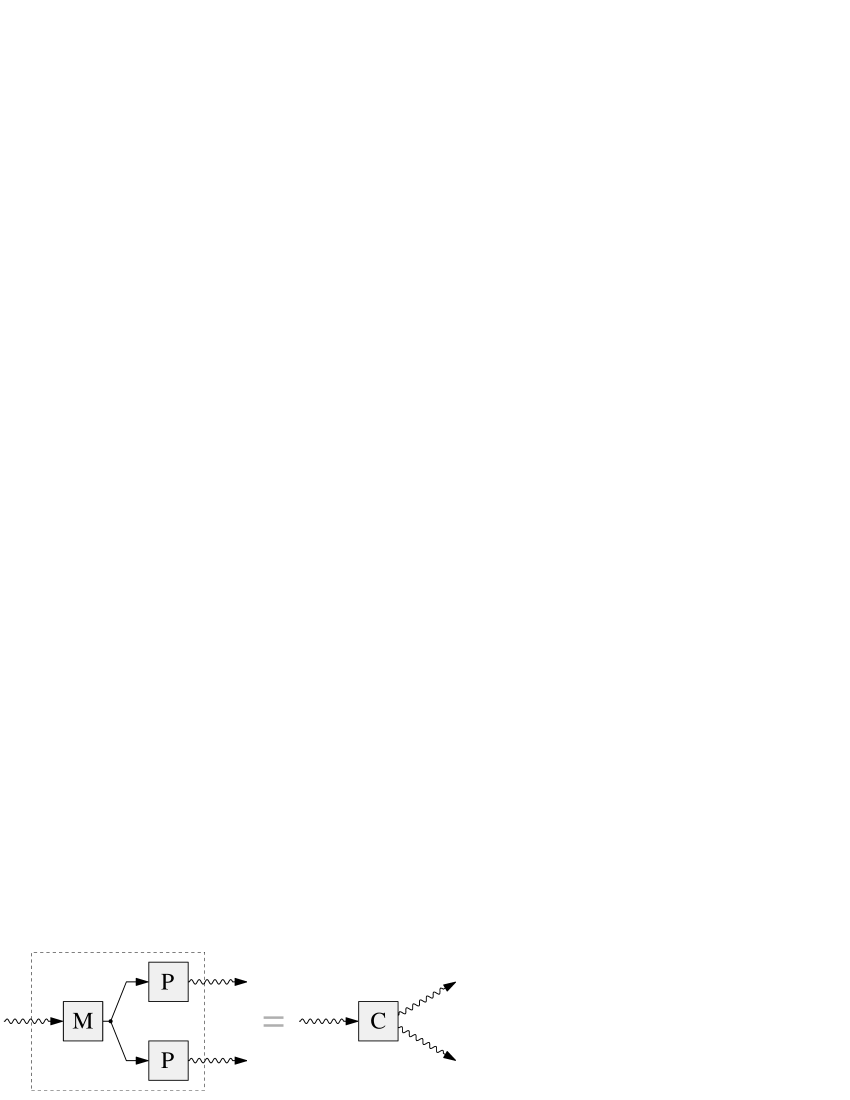
Figure 3.1: Making a copier from a “classical teleportation” line

3.2 The Joint Measurement

This is the task of combining two separate measuring devices into a single device, or the “simultaneous measurement” of two quantum observables $A$ and $B$. Thus a joint measuring device “$A\&B$” is a device giving a pair $(a,b)$ of classical outputs each time it is operated, such that $a$ is a possible output of $A$, and $b$ is a possible output of $B$. We require that the statistics of the $a$ outcomes alone is the same as for device $A$, and similarly for $B$. Note that once again our criterion is statistical, and can be tested without recourse to counterfactual conditionals such as “the result which would have resulted if $B$ rather than $A$ had been measured on this particular quantum particle”.

Many quantum observables are not jointly measurable in this sense. The most famous examples, position and momentum, different components of angular momentum, and positions of a free particle at different times, are probably contained in every quantum mechanics course. Hence the impossibility of joint measurements is nothing but a precise statement of an aspect of “complementarity”.

Nevertheless, a joint measurement device for any of these could readily constructed given a functioning quantum copier (see Figure 3.2): one would simply run the copier C on the quantum system, and then apply the two given measuring devices, A and B, to the copies. It is easy to see that the definition of the copier then guarantees that the statistics of $a$ and $b$ separately come out right. In other words, a copier can be seen as a universal joint measuring device.

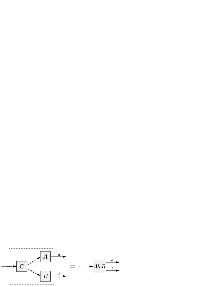
Figure 3.2: Getting joint measurements from a copier

3.3 Bell’s Telephone

This is not named after a certain phone company, but after John S. Bell, who never proposed it in this form, but might have. It refers to the project of installing superluminal communication using only correlations of the type tested by Bell’s inequalities. Without going into details for the moment, the basic setup would consist of a source producing pairs of particles, and sending one member of the pair to each of the two communicating parties, conventionally named “Alice” and “Bob”. Each of them has a collection of different measuring devices to choose from, and the idea is for Alice to do something which creates a noticeable change in the probabilities measured by Bob. Clearly, this is a paradoxical task, because no particle or other physical carrier of information actually goes from Alice to Bob. Therefore, if only the particles move sufficiently far apart, this device would transmit superluminally.

It is maybe useful to point out here a common confusion concerning such superluminal effects, which sometimes even afflicts otherwise reliable professional writers. The mistake is usually spotted easily by a device I call the “Ping Pong Ball Test”. It goes like this:

Take an author’s explanation of Bell’s inequalities, and substitute “ping pong balls” for every quantum particle. Then if whatever the author is selling as paradoxical, remains true, he/she hasn’t understood a thing.

Here is an example: imagine a box containing a ping pong ball, which can be separated into two parts, without looking at the ball. One part is shipped to Tokyo or Alpha Centauri, without looking inside. Then if I open the other box I know instantly, i.e., “at superluminal speed” whether the ball is at the distant location or not. Of course, that is true, but hardly paradoxical, and totally useless for sending a message either way. To repeat: there is nothing paradoxical in statistical correlations per se between distant systems with a common past, even if the correlation is perfect.

If Alice wants to send a message to Bob, correlations between any two measuring devices are useless, because they cannot even be detected without comparing the results, which requires exactly the communication the Telephone was intended for. Only if something Alice does has an effect on measuring results at Bob’s end we can speak of communication. The only thing Alice can do in the standard setup is to choose a measuring device, and Bell’s Telephone can be said to work if these choices have an influence on the probabilities measured by Bob (who has no access to Alice’s measuring results). If there is no physical system traveling from Alice to Bob, however, this will be impossible.

To be sure, this can hardly be counted as an impossible machine of quantum mechanics, since the argument has nothing to do with quantum theory. What makes it fit into the hierarchy described here is the following: if we assume that Bob has a joint measuring device for two yes/no measurements, and Bell’s inequality is violated, we can design a strategy for Alice to send signals to Bob with better than chance results. Hence the joint measurement of suitable observables can be a device sufficiently strong to achieve a task forbidden by Causality, and is hence impossible in general. This is the last construction in the hierarchy of impossible machines mentioned at the beginning of this section.

The proof of this step amounts to yet another derivation of Bell’s inequalities, but since it emphasizes the communication aspect it fits well into our context, and we will at least sketch it. This step will be rather more technical than the rest of this section, but does not require any quantum theory. The argument can be skipped without loss to later sections.

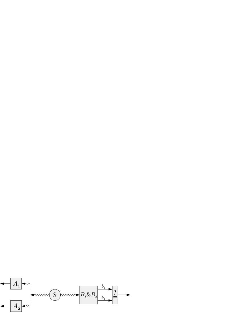
Figure 3.3: Building Bell’s Telephone from a joint measurement

So let us assume that Alice and Bob each have at their disposal two measuring devices, say $A_{1},A_{2}$ and $B_{1},B_{2}$, respectively. Each of these can either give the result $+1$ or $-1$. We will denote by ${\mathbb{P}}(a,b\mid A_{i},B_{j})$ the probability for Alice to get $a$, and Bob to get $b$, in a correlation experiment in which Alice used measuring device $A_{i}$ and Bob uses $B_{j}$. By

$$C(A_{i},B_{j})=\sum_{a,b}ab\ {\mathbb{P}}(a,b\mid A_{i},B_{j})$$

we will denote the correlation coefficient, which lies between $-1$ and $+1$. The combination

$$\beta=C(A_{1},B_{1})+C(A_{1},B_{2})+C(A_{2},B_{1})-C(A_{2},B_{2})$$ (3.1)

carries special significance, as we will see below. Because the inequality “$\beta\leq 2$” is known as the Bell inequality, we will call $\beta$ the Bell correlation for this choice of four observables. It is a quantity directly accessible to experiment. Note that usually Bob cannot tell from his data which apparatus ($A_{1}$ or $A_{2}$) Alice chose. This is reflected by the equation

$$\sum_{a}{\mathbb{P}}(a,b\mid A_{1},B_{j})=\sum_{a}{\mathbb{P}}(a,b\mid A_{2},B_{j})\equiv{\mathbb{P}}(b\mid B_{j})\;,$$

and borne out by all known experimental data. Now suppose Bob has a joint measuring device for his $B_{1}$ and $B_{2}$, which we will denote by $B_{1}\&B_{2}$, which produces pair outcomes $(b_{1},b_{2})$ (see Figure 3.3). We can then determine the probabilities $p_{i}(a_{i},b_{1},b_{2})={\mathbb{P}}(a_{i},(b_{1},b_{2})\mid A_{i},B_{1}\&B_{2})$. The condition that this is really a joint measurement is expressed by the equations

$$\sum_{b_{1}}p_{i}(a_{i},b_{1},b_{2}) = {\mathbb{P}}(a_{i},b_{2}\mid A_{i},B_{2})\quad\hbox{and }$$ (3.2)

$$\sum_{b_{2}}p_{i}(a_{i},b_{1},b_{2}) = {\mathbb{P}}(a_{i},b_{1}\mid A_{i},B_{1})\;,$$ (3.3)

each for $i=1,2$. The basic rule for the information transmission is the following:

Alice encodes the bit she wants to send by either choosing apparatus $A_{1}$ or apparatus $A_{2}$. Then Bob looks at his readout and interprets it as “$A_{1}$”, whenever the two displays coincide ($b_{1}=b_{2}$) and as “$A_{2}$”, if they are different.

We can then estimate the probability $p_{\rm ok}$ for Bob to be right, assuming that the choices $A_{1}$ and $A_{2}$ are made with the same frequency. Assume first that Alice chooses $A_{1}$. Then Bob is right with probability

$$\sum_{a_{1},b_{1},b_{2}}\left|\frac{b_{1}+b_{2}}{2}\right|\ |a_{1}|\ p_{1}(a_{1},b_{1},b_{2})\;,$$

where the first factor takes into account the condition $b_{1}=b_{2}$, and the second is introduced for later convenience. Combining this with the second term of this kind for Alice’s choice $A_{2}$, and taking into account the probability $1/2$ for these choices we get the overall probability $p_{\rm ok}$ for Bob to be correct as

$$p_{\rm ok} = \frac{1}{2}\sum_{a_{1},b_{1},b_{2}}\left|\frac{b_{1}+b_{2}}{2}\right|\ |a_{1}|\ p_{1}(a_{1},b_{1},b_{2})$$ (3.4)

$$\qquad+\frac{1}{2}\sum_{a_{2},b_{1},b_{2}}\left|\frac{b_{1}-b_{2}}{2}\right|\ |a_{2}|\ p_{2}(a_{2},b_{1},b_{2})$$

$$\geq \frac{1}{4}\sum_{a_{1},b_{1},b_{2}}(b_{1}+b_{2})a_{1}\;p_{1}(a_{1},b_{1},b_{2})$$

$$\qquad+\frac{1}{4}\sum_{a_{2},b_{1},b_{2}}(b_{1}-b_{2})a_{1}\;p_{2}(a_{2},b_{1},b_{2})$$

$$= \frac{1}{4}\Bigl{(}C(A_{1},B_{1})+C(A_{1},B_{2})+C(A_{2},B_{1})-C(A_{2},B_{2})\Bigr{)}$$

$$= \frac{\beta}{4}\;.$$

Bob is right with better than chance, if $p_{\rm ok}>1/2$, which by this computation can be guaranteed as soon as $\beta>2$, i.e., as soon as the classical Bell inequality (in Clauser-Horne-Shimony-Holt form [6]) is violated. But this is indeed the case in the experiments conducted to determine $\beta$ (e.g., [11]), which give roughly $\beta\approx 2\sqrt{2}\approx 2.8$. If we believe these experiments, the only conclusion is that the joint measurability of the $B_{1}$ and $B_{2}$ used in the experiment would be sufficient to make Bell’s Telephone work, which was our claim.

3.4 Entanglement, mixed state analyzers, and correlation resolvers

Violations of Bell’s inequalities can also be seen to prove the existence of a new class of correlations between quantum systems, known as entanglement. This concept is as fundamental to the field of quantum information theory as the idea of quantum information itself. So rather than organizing this introduction as an answer to the the question “why quantum information is different from classical information”, we could have followed the line “why entanglement is different from classical correlation”. There are impossible machines in this line of approach, too, and we will now describe briefly how they fit in.

Consider a correlation experiment of the kind used in Bell’s inequalities (see Section 3.3). If Bob looks at his particles, and makes measurements on them without any communication from Alice, he will find that their statistics are described by a certain mixed state. It must be mixed, because if he now listens to Alice and sorts his particles according to Alice’s measuring results, he will get two subensembles, which are in general different. In the usual ideal 2-qubit situation, in which one gets the maximal violation of Bell’s inequalities, these subensembles are described by pure states.

This is very satisfying for people who see the occurrence of mixed states in quantum mechanics merely as a result of ignorance, as opposed to the deeper kind of randomness encoded in pure states. This view usually comes with an individual state interpretation of quantum mechanics, by which each individual system can be assigned a pure state (a single vector in Hilbert space), and a general preparing procedure is not just given by its density matrix, but by a specific probability distribution of pure states. Let us call a mixed state analyzer a hypothetical device, which can see the difference, i.e., a measuring device whose output after many measurements on a given ensemble is not just a collection of expectations of quantum observables, but the distribution of pure states in the ensemble. In the case of a correlation experiment, where Bob sees a mixed state only because he is ignorant about Alice’s results, this machine would find for him the decomposition of his mixed state into two pure states.

The problem is, of course, that Alice has several choices of measuring devices, and that the decomposition of Bob’s mixed state depends, accordingly, on Alice’s choice. Hence she could signal to Bob, and we would have another instance of Bell’s Telephone. There would be a way out if Joint Measurements were available (to Alice in this case): then we could say that the two decompositions were just the first step in an even finer decomposition, a further reduction of ignorance, which would be brought to light if Alice would apply her joint measurement. Presumably the mixed state analyzer would then yield this finer decomposition, because the operation of this device would not depend on how closely Alice cares to look at her particles.

But just as two quantum observables are often not jointly measurable, two decompositions of mixed states often have no common refinement (Actually, in the formalism of quantum theory these are two variants of the same theorem). In particular, the two decompositions belonging to Alice’s choices in an experiment demonstrating a violation of Bell’s inequalities have no common refinement, and any mixed state analyzer could be used for superluminal communication in this situation.

Another device, which is suggested by the individual state interpretation arises from a naive extrapolation of this view to the parts of a composite system: if every single system can be assigned a pure state, a composite system could be assigned a pair of pure states, one for each subsystem. A correlated state should therefore be given by a probability distribution of such pairs. A device, which represents an arbitrary state of a composite system as a mixture of uncorrelated pure product states might be called a correlation resolver. It could be built given a classical teleportation line: when one applies the teleportation to one of the subsystems, and conditions on the classical measurement results of the intermediate stage, one gets precisely a representation of an arbitrary state in this form. But it is easy to see that any state which can be so analyzed automatically satisfies all Bell-type inequalities, and hence once again the experimental violations of Bell’s inequalities show that such a correlation resolver cannot exist. Hence we have here a second line of reasoning for showing the No-Teleportation Theorem: a teleportation device would allow classical correlation resolution, which is shown to be impossible by the Bell experiments.

The distinction of resolvable states and their complement is one of the starting points of entanglement theory, where the “resolvable” states are called “separable”, or “classically correlated”, and all others or simply “entangled”. For more detailed treatment and an up-to date overview, the reader is referred to the article by the Horodecki family in this volume.

Without going into philosophical discussions on the foundations of quantum mechanics, I should comment briefly on the individual state interpretation, which has suggested the two impossible machines discussed in this subsection. First, this view is not at all uncommon, and it is quite possible to read some passages from the Masters of the Copenhagen Interpretation as an endorsement of this view. Secondly, if we define a hidden variable theory as a theory in which individual systems are described by classical parameters, whose distribution is responsible for the randomness seen in quantum experiments, we have no choice but to call the individual state interpretation a hidden variable theory. The hidden variable in this theory is usually denoted by $\psi$. And sure enough, as we have just pointed out, it has all the difficulties with locality such a theory is known to have on general grounds. Thirdly, avoiding an individual state interpretation, and with it some of its misleading intuitions, is easy enough. In practice this is done anyhow, by concentrating on those aspects of the theory, which have some direct statistical meaning, not involving hypothetical, and usually impossible devices. This common ground is the statistical interpretation of quantum mechanics, in which states (pure or mixed) are the analogs of classical probability distributions, and are not seen as a property of the individual system, but of a specific way of preparing the systems.

Chapter 4 Possible Machines

4.1 Operations on multiple inputs

The No-Teleportation Theorem derived in the previous chapter says that there is no way to measure a quantum state in such a way that the measuring results suffice to reconstruct the state. At first sight this seems to deny that the notion of “quantum states” has an operational meaning at all. But there is no contradiction, and we will resolve the apparent conflict in this subsection, if only to sharpen the statement of the No-Teleportation Theorem.

Let us recall the operational definition of quantum states, according to the statistical interpretation of quantum mechanics. A state is the description of a way of preparing quantum systems, in all aspects relevant to computing expectation values. We might also say that it is the assignment of an expectation value to every observable of the system. So to the extent that expectation values can be measured, it is possible to determine the state by testing it on sufficiently many observables. What is crucial, however, is that even the determination of a single expectation value is a statistical measurement. Hence it requires a repetition of the experiment many times, using many systems prepared according to the same procedure. In contrast, the above description of teleportation demands that it works with a single quantum system as input, and that the measuring device does not accumulate results from several input systems. Expressed in the current jargon: teleportation is required to be a one-shot operation. Note that this does not contradict our statistical criteria for success of teleportation and other devices, which involve a statistics of independent “single shots”.

If we have available many identically prepared systems, many operations which are otherwise impossible, become easy. Let us begin with classical teleportation. Its multi-input analog is the state estimation problem: how can we design a measurement operating on samples of many (say, $N$) systems from the same preparing device, such that the measuring result in each case is a collection of classical parameters forming a hermitian matrix, which on average is close to the density matrix describing the initial preparation. This is symbolized in Figure 4.1 (with the box T omitted for the moment): the box P at the end would be a repreparation of systems according to the estimated density matrix. The overall output will then be a quantum system, which can be directly compared with the inputs in statistical experiments. It is clear that the state cannot be determined exactly from a sample with finite $N$, but the determination becomes arbitrarily good in the limit $N\to\infty$. Optimal estimation observables are known in the case when the inputs are guaranteed to be pure [7], but in the case of general mixed states there are no clear cut theorems yet, partly due to the fact that it is less clear what “figure of merit” best describes the quality of such an estimator.

Given a good estimator we can, of course, proceed to good cloning by just repeating the re-preparation P as often as desired. The surprise here [8] is that if only a fixed number $M$ of outputs is required, it is possible to get better clones by devices staying entirely in the quantum world than by going via classical estimation. Again, the problem of optimal cloning is fully understood for pure states [9], but work has only just begun to understand the mixed state case.

Another operation, which becomes accessible in this way is the Universal Not operation, assigning to each pure qubit state the unique pure state orthogonal to it. Like time reversal, this is just a special case an anti-unitarily implemented symmetry operation. In this case, the strategy using a classical estimation as an intermediate step can be shown to be optimal [10]. In this sense “Universal Not” is a harder task than “cloning”.

Figure 4.1: Classical Teleportation on multiple inputs, or state estimation

More generally, we can look at schemes as in Figure 4.1, with T representing any transformation of the density matrix data, whether or not this transformation corresponds to a physically realizable transformation of quantum states. A further interesting application is to the purification of states. In this problem it is assumed that the input states were once pure, but later corrupted in some noisy environment (the same for all inputs). The task is to reconstruct the original pure states. Usually, the the noise corresponds to an invertible linear transformation on the density matrices, but its inverse is not a possible operation, because it takes some density matrices to operators with negative eigenvalues. So the reversal of noise is not possible by a one-shot device, but is easy to a high accuracy when many equally prepared inputs are available. In the simplest case of a so-called depolarizing channel this problem is well understood [13], also in the version requiring many outputs as in the optimal cloning problem [14].

4.2 Quantum Cryptography

It may seem impossible to find applications of impossible machines. But that is not quite true: sometimes the impossibility of a certain task is precisely what is called for in an application. A case in point is cryptography: here one tries to make deciphering of a code impossible. So if we can design a code, whose breaking would require one of the machines in the previous section we could guarantee its security with the certainty of Natural Law. This is precisely what Quantum Cryptography sets out to do. Because only small quantum systems are involved it is one of the “easiest” applications of quantum information ideas, and was indeed the first to be realized experimentally. For a detailed description we refer to the article by Weinfurter and Zeilinger. Here we just describe in what sense it is the application of an impossible machine.

As always in cryptography, the basic situation is that two parties, Alice and Bob, say, want to communicate without giving an Evil Eavesdropper, conventionally named Eve, a chance to listen in. What classical eavesdroppers do is to tap the transmission line, make a copy of what they hear for later analysis, and otherwise let the signal pass undisturbed to the legitimate receiver (Bob). But if the signal is quantum, the No-Cloning Theorem tells us that faithful copying is impossible. So either Eve’s copy or Bob’s copy is corrupted. In the first case Eve won’t learn anything, and there was no eavesdropping anyway. In the second case Bob will know something may have gone wrong, and will tell Alice that they must discard that part of the secret key they were exchanging. Of course, intermediate situations are possible, and one has to show very carefully that there is an exact tradeoff between the amount of information Eve can get and the amount of perturbation she must inflict on the channel.

4.3 Entanglement assisted Teleportation

This is arguably the first major discovery in the field of quantum information. The No-Cloning and No-Teleportation Theorems, although not formulated in such terms, would hardly have come as a surprise to people working on foundations of quantum mechanics in the sixties, say. But entanglement assistance was really an unexpected turn. It was first seen by Bennett, Brassard, Crepeau, Jozsa, Peres, and Wootters [12], who also coined the term “teleportation”. It is gratifying to see, though hardly a surprise on the same scale, that this prediction of quantum mechanics has also been implemented experimentally. The experiments are another interesting story, which will no doubt be told much better in the article of Weinfurter and Zeilinger, who represent one team in which major breakthrough in this regard was achieved.

The teleportation scheme is shown in Figure 4.2. What makes it so surprising is that it combines two machines whose impossibility was discussed in the previous section: omitting the entanglement distribution (the lower half of Figure 4.2) we get the impossible process of classical teleportation. On the other hand, if we omit the classical channel, we get an attempt to transmit information on correlations alone, i.e., a version of Bell’s telephone.

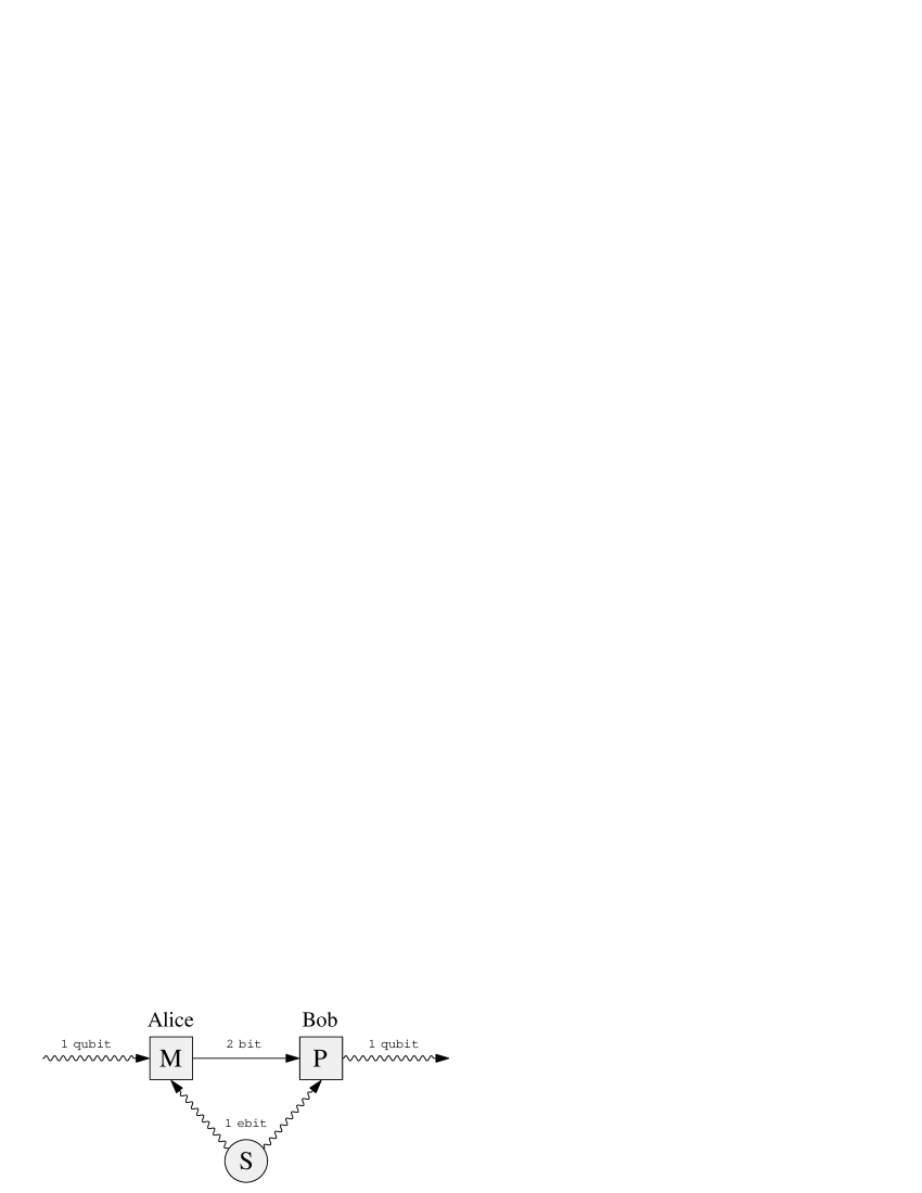
Figure 4.2: Entanglement assisted Teleportation

Since the time dimension is not represented in this diagram, let us consider the steps in due order. The first step is that Alice and Bob each receive one half of an entangled system. The source can be a third party or can be Bob’s lab. The last choice is maybe best for illustrative purposes, because it makes clear that no information is flowing from Alice to Bob at this stage. Alice is next given the quantum system whose state (unknown to her) she is to teleport. Alice then makes a measurement on the system combined out of the input and her half of the entangled system. She sends the results via a classical channel to Bob, who uses them to adjust the settings on his device, which then performs some unitary transformation on his half of the entangled system. The resulting system is the output, and if everything is chosen in the right way, these output systems are indeed statistically indistinguishable from the outputs. To see just how entangled state S, measurement M and repreparation P have to be chosen, requires the mathematical framework of quantum theory. In the standard example one teleports the state of one qubit, using up one maximally entangled two qubit system (jargon: “1 ebit”) and sending two classical bits from Alice to Bob. A general characterization of the teleportation schemes for qubits and higher dimensional systems is given below in Section 4.3.

4.4 Superdense Coding

It is easy to see, and in fact a commonplace occurrence that classical information can be transmitted on quantum channels. For example, one bit of classical information can be coded in every 2 level system, like, e.g., the polarization degree of freedom of a photon. It is not entirely trivial to prove, but hardly surprising that one cannot do better than “1 bit per qubit”. Can we beat this bound using the idea of entanglement assistance? It turns out that one can. In fact one can double the amount of classical information carried by a quantum channel (“2 bits per qubit”). Remarkably, the setups for doing this are closely related to teleportation schemes, and in the simplest cases Alice and Bob just have to swap their equipment for entanglement assisted teleportation. This is explained in detail in Section 4.3.

4.5 Quantum Computation

Again, we will be very brief on this subject, although it is certainly central to the field. After all, it is partly the promise of a fantastic new class of computers, which has boosted the interest in quantum information in recent years. But since in this book computation is covered in the article by Beth, we will only make a few remarks, connecting it to the theme of possible versus impossible machines.

So can Quantum Computers perform otherwise impossible tasks? Not really, because in principle we can solve the dynamical equations of quantum mechanics on a classical computer, and simulate all the results. Hence classical unsolvable problems like the Halting Problem for Turing Machines, or the Word Problem in group theory cannot be solved on quantum computers either. But this argument only shows the possibility of emulating all quantum computations on a classical computer, and omits the fact that the efficiency of this procedure may be terrible. The great promise of Quantum Computation lies therefore in the reduction of running time, in the case of Shor’s factorization algorithm [33] from exponential to polynomial time. This reduction is comparable to replacing the task of counting all the way up to a 137 digit number by just having to write it. No matter what the constants are in the growth laws for the computing time (and they will probably not be very favorable for the quantum contestant), the polynomial time is going to win if we are really interested in factoring very large numbers.

A word of caution is necessary here concerning the impossible/possible distinction. While it is true that no polynomial time classical factoring algorithm is known, and this is what counts from a practical point of view, there is no proof that no such algorithm exists. This is a typical state of affairs in complexity theory, because the non-existence of an algorithm is a statement about the rather unwieldy set of all Turing machine programs. A proof by inspecting all of them is obviously out, so it would have to be based on some principle of “conservation of difficulties”, which rarely exists for real life problems. One problem in which this is possible is identifying which (unique) element of a large list has a certain property (“needle in a haystack”). In this case the obvious strategy of inspecting every element in turn can be shown to be the optimal classical one, and has a running time proportional to the length $N$ of the list. But Grover’s quantum algorithm [1] does it in the order of $\sqrt{N}$ steps, an amazing gain even if it is not exponential. Hence there are problems for which quantum computers are provably faster than any classical computer.

So what makes it work? This is not so easy to answer, even after working through Shor’s algorithm and verifying the claim of exponential speedup. Massive entanglement is used in the algorithm, so this is certainly one important element. Then there is a technique known as quantum parallelism, in which a quantum computation is run on a coherent superposition of all possible classical inputs, and in a sense, all values of a function are computed simultaneously. A catchy paraphrase attributed to D. Deutsch is to call this a computation in the parallel worlds of the many-worlds interpretation.

But perhaps the best way to find out what powers quantum computation is to to turn it around and to really try the classical emulation. The practical difficulty which then becomes apparent immediately is that Hilbert space dimensions grow extremely fast. For $N$ qubits (two-level systems) one has to operate in a Hilbert space of $2^{N}$ dimensions. The corresponding space of density matrices has $2^{2N}$ dimensions. For classical bits one has instead a configuration space of $2^{N}$ discrete points, and the analogue of the density matrices, the probability densities live in a merely $2^{N}$ dimensional space. Brute force simulations of the whole system therefore tend to grind to a halt already on fairly small systems. Feynman was the first to turn this around: maybe only a quantum system can be used to simulate a quantum system, and maybe, while we are at it, we can go beyond simulation and do some interesting computations as well. So putting it positively: in a quantum system we have exponentially more dimensions to work with: there is lots of room in Hilbert space. The added complexity of quantum vs. classical correlations, i.e., the phenomenon of entanglement, is also a consequence of this.

But it is not so easy to use those extra dimensions. For example, for transmission of classical information an $N$-qubit system is no better than a classical $N$-bit system. Only the entanglement assistance of superdense coding brings out the additional dimensions. Similarly, quantum computers do not speed up every computation, but are only good at specific tasks where the extra dimensions can be brought into play.

4.6 Error correction

Again we will only make a few remarks related to the possible/impossible theme, and refer the reader to T. Beth’s article in this volume for a deeper discussion. First of all, error correction is absolutely crucial for the implementation of quantum computers. Very early in the development the suspicion was raised that exponential speedup was only possible, if all component parts of the computer were realized with exponentially high (hence practically unattainable) precision.

In a classical computer the solution to this problem is digitization: every bit is realized by a bistable circuit, and any deviation from the two wanted states is restored by the circuit at the expense of some energy and with some heat generation. This works separately for every bit, so in a sense every bit has its own heat bath. But this strategy will not work for quantum computers: to begin with there is now a continuum of pure states which would have to be stabilized for every qubit, and secondly, one heat bath per qubit would quickly destroy entanglement, and hence make the quantum computation impossible. There are many indications that entanglement is indeed more easily destroyed by thermal noise and other sources of errors, summarily referred to as decoherence. For example, a Gaussian channel (this is a special type of infinite dimensional channel) has infinite capacity for classical information, no matter how much noise we add. But its quantum capacity drops to zero, if we add more classical noise than specified by the Heisenberg uncertainty relations [16].

A standard technique for stabilizing classical information is redundancy: just send a classical bit three times, and decide at the end by majority vote which bit to take. It is easy to see that this reduces the probability of error from order $\varepsilon$ to order $\varepsilon^{2}$. But quantum mechanically this procedure is forbidden by the No-Cloning Theorem: We simply cannot make three copies to start the process.

Fortunately quantum error correction is possible in spite of all these doubts [2]. It also works by distributing the quantum information over several parallel channels, but does this in a much more subtle way than copying. Using five parallel channels one can get a similar reduction of errors from order $\varepsilon$ to order $\varepsilon^{2}$ [3]. Much more has been done, but many open problems remain, for which I refer once again to the article by Beth.

Chapter 5 A Preview of the Quantum Theory of Information

Before we go on in the next section to turn some of the heuristic descriptions of the previous sections into rigorous mathematical statements, I will try to give a flavor of the theory to be constructed, and of its motivations and current state of development.

Theoretical physics contributes to the field of Quantum Information Processing in two distinct though interrelated ways. On the one hand, it is necessary to build theoretical models of the systems which are being set up experimentally as candidates for quantum devices. Of course, any such system will have very many degrees of freedom, of which only very few are singled out as the “qubits” on which the quantum computation is performed. Hence it is necessary to analyze to what degree and on what time scales it is justified to treat the qubit degrees of freedom separately, and with what errors the desired quantum operation can be realized in the given system. These questions are crucial for the realizations of all quantum devices, and require specialized in-depth knowledge of the appropriate theory, e.g., quantum optics, solid state theory, or quantum chemistry (in the case of NMR quantum computing). However, these problems are not what we want to look at in this article.

We are concerned here with another kind of theoretical work, which could be called the Abstract Quantum Theory of Information. Recall the arguments in Section 2, where the possibility of translating between different carriers of (classical) information was taken as the justification for looking at an abstracted version, the classical Theory of Information, as founded by Shannon. While it is true that quantum information cannot be translated into this framework, and is hence a new kind of information, translation is often possible (at least in principle) between different carriers of quantum information. Therefore, we can make a similar abstraction in the quantum case. To this abstracted theory all qubits are the same, whether they are realized as polarization of photons, nuclear spins, excited states of ions in a trap, modes of a cavity electromagnetic field, or whatever other realization may be feasible. A large amount of work is currently devoted to this abstract branch of quantum information theory, so I will list some of the reasons for this effort.

• Abstract quantum theoretical reasoning is how it all started. In the early papers of Feynman and Deutsch, and the papers by Bennett and co-workers, it is the structure of quantum theory itself, which opens up all those new possibilities. No hint from experiment and no particular theoretical difficulty in the description of concrete systems prompted this development. Since the technical realizations are lagging behind so much, the field will probably remain “theory driven” for some time to come.

• If we want to transfer ideas from the Classical Theory of Information to the Quantum Theory, we will always get abstract statements. This works quite well for importing good questions. Unfortunately, however, the answers are most of the time not transferred so easily.

• The reason for this difficulty with importing classical results is that some of the standard probabilistic techniques, such as conditioning, do not work in quantum theory, or work only sporadically. This is the same problem that the Statistical Mechanics of quantum many-particle systems is facing in comparison to its classical sister. The cure can only be the development of new, genuinely quantum techniques. Preferably these should work in the widest (hence most abstract) possible setting.

• One of the fascinating aspects of quantum information is that features of quantum mechanics, which were formerly seen only as paradoxical or counter-intuitive are now turned into an asset: these are precisely the features one is trying to utilize now. But this means that naive intuitive reasoning tends to come to wrong results. Until we know much more about Quantum Information we will need rigorous guiding from a solid conceptual and mathematical foundation of the theory.

• When we take as a selling point for, say Quantum Cryptography, that secrets are protected “with the security of Natural Law”, the argument is only as convincing as the proof reducing this claim to first principles. Clearly this requires abstract reasoning, because it must be independent of the physical implementation of the device the eavesdropper uses. It must also be completely rigorous in the mathematical sense.

• Because it does not care about the physical realization of its “qubits”, the Abstract Quantum Theory of Information is applicable to a wide range of seemingly very different system. Consider, for example some abstract quantum gate like the “controlled not” (C-NOT). From the abstract theory we can hope to get relevant quality criteria such as the minimal fidelity with which this has to be implemented for some algorithm to work. So systems of quite different type can be checked according to the same set of criteria, and a direct competition becomes possible (and interesting) between different branches of experimental physics.

So what will be the basic concepts and features of the emerging Quantum Theory of Information? The information theoretical perspective typically generates questions like

How can a given task of quantum information processing be performed optimally with the given resources?

We have already seen a few typical tasks of quantum information processing in the previous section and, of course, there are more. Typical resources for cryptography, quantum teleportation, and dense coding are entangled states, quantum channels and classical channels. In error correction and computing tasks, resources are the size of quantum memory, and the number of quantum operations. Hence all these notions take on a quantitative meaning.

For example, in entanglement assisted teleportation the entangled pairs are used up (one maximally entangled qubit pair is needed for every qubit teleported). If we try to run this with less than maximally entangled states, we may still ask, how many pairs from a given preparation device are needed per qubit to teleport a message of many qubits, say, with error less than $\varepsilon$. This quantity is clearly a measure of entanglement. But other tasks may lead to different quantitative measures of entanglement. Very often it is possible to find inequalities between different measures of entanglement, and establishing these is again a task of quantum information theory.

The direct definition of the entanglement measure based on teleportation, or the quantum information capacity of a channel, and many similar quantities require an optimization with respect to all codings and decodings of asymptotically long quantum messages, which is extremely hard to evaluate. In the classical case, however, there is a simple formula for the capacity of a noisy channel, called Shannon’s Coding Theorem, which allows us to compute the capacity directly from the transition probabilities of a channel. Finding quantum analogs of the Coding Theorem (and similar formulas for entanglement resources) is still one of the great challenges in quantum information theory.

Chapter 6 Elements of Quantum Information Theory

It is probably too early to write a definitive account of Quantum Information Theory – there are simply too many open questions. But the basic concepts are clear enough, and it will be the task of the remainder of this article to explain them, and use these sharp definitions to state some of the interesting open problems in the field. In the limited space available this cannot be done in textbook-style, with many examples and full proofs (or even full references) of all the things used on the way. So I will try to emphasize the main lines, and to set up the basic definitions using as few primitive concepts as possible. For example, the capacities of a channel for either classical or quantum information will be defined on exactly the same pattern. This will make it easier to establish the relations between these concepts.

The following pages begin with material which every physicist knows from quantum mechanics courses, although maybe not in this form. We need to go over it, though, in order to establish notation.

6.1 Systems and States

The systems occurring in the theory can be either quantum or classical, or can be hybrids composed of a classical and a quantum part. Therefore, we need a mathematical framework covering all these cases. A good choice is to characterize each type of systems by its algebra of observables. In this article all observable algebras will be taken to be finite dimensional for simplicity. Extensions to infinite dimension are mostly straightforward, though, and in fact a strength of the algebraic approach to quantum theory is that it deals not just with infinite dimensional algebras, but also with systems of infinitely many degrees of freedom as in quantum field theory [34, 35] and statistical mechanics [17].

The first main type of systems are purely classical systems, whose observable algebra is commutative, and can hence be considered as a space of complex valued functions on a set $X$. Our standing finiteness assumption requires that $X$ is a finite set, and the observable algebra ${\cal A}$ will be ${\cal C}(X)$, the space of all functions $f:X\to{\mathbb{C}}$. A single classical bit corresponds to the choice $X=\{0,1\}$. On the other hand, a purely quantum system is determined by the choice ${\cal A}={\cal B}({\cal H})$, the algebra of all bounded linear operators on the Hilbert space ${\cal H}$. The finiteness assumption requires that ${\cal H}$ has finite dimension $d$, so ${\cal A}$ is just the space ${\cal M}_{d}$ of complex $d\times d$-matrices. A qubit is given by ${\cal A}={\cal M}_{2}$.

The basic statistical interpretation of the observable algebra is the same in the quantum and classical case, and hinges on the cone of positive elements in the algebra. Here $Y$ is called positive (in symbols $Y\geq 0$) if it can be written in the form $Y=X^{*}X$. Then $Y\in{\cal M}_{d}$ is positive, exactly if it is given by a positive semidefinite matrix, and $f\in{\cal C}(X)$ is positive iff $f(x)\geq 0$ for all $x$. In any observable algebra ${\cal A}$, we will denote by ${\rm 1\mkern-5.4muI}\in{\cal A}$ the identity element.

A state $\Phi$ on ${\cal A}$ is a positive normalized linear functionals on ${\cal A}$. That is, $\Phi:{\cal A}\to{\mathbb{C}}$ is linear, with $\Phi(X^{*}X)\geq 0$ and $\Phi({\rm 1\mkern-5.4muI})=1$. Each state describes a way of preparing systems in all the details, which are relevant for subsequent statistical measurements on the systems. The measurements are described by assigning to each outcome of a device an effect $F\in{\cal A}$, i.e., an element with $0\leq F\leq{\rm 1\mkern-5.4muI}$. The prediction of the theory for the probability of that outcome, measured on systems prepared according to the state $\rho$ is then $\rho(F)$.

For explicit computations we will often need to expand states and elements of ${\cal A}$ in a basis. The standard basis in ${\cal C}(X)$ consists of the functions $e_{x},x\in X$, such that $e_{x}(y)=1$ for $x=y$ and zero otherwise. Similarly, if $\phi_{\mu}\in{\cal H}$ is an orthonormal basis of the Hilbert space of a quantum system, we denote by $e_{\mu\nu}=|e_{\mu}\rangle\langle e_{\nu}|\in{\cal B}({\cal H})$ the corresponding “matrix units”. Then a state $p$ on the classical algebra ${\cal C}(X)$ is characterized by the numbers $p_{x}\equiv p(e_{x})$, which form a probability distribution on $X$, i.e., $p(x)\geq 0$ and $\sum_{x}p(x)=1$. Similarly, a quantum state $\rho$ on ${\cal B}({\cal H})$ is given by the numbers $\rho_{\mu\nu}\equiv\rho(e_{\nu\mu})$, which form the so-called density matrix. If we interpret them as the expansion coefficients of an operator $\widehat{\rho}=\sum_{\mu\nu}\rho_{\mu\nu}e_{\mu\nu}$, the density operator of $\rho$, we can also write $\rho(A)={\mathop{\rm tr}\nolimits}(\widehat{\rho}A)$.

A state is called pure, if it is extremal in the convex set of all states, i.e., if it cannot be written as a convex combination $\lambda\rho^{\prime}+(1-\lambda)\rho^{\prime\prime}$ of other states. These are the states, which contain as little randomness as possible. In the classical case, the only pure states are those concentrated on a single point $z\in X$, i.e., $p_{z}=1$, or $p(f)=f(z)$. The pure states in the quantum case are determined by “wave vectors” $\psi\in{\cal H}$ such that $\rho(A)=\langle\psi,A\psi\rangle$, resp. $\widehat{\rho}=|\psi\rangle\langle\psi|$. Thus in the simplest case of a classical bit there are just two extreme points, whereas in the case of a qubit the extreme points form a sphere in three dimensions which are given by the expectations of the three Pauli matrices:

$$\widehat{\rho} = \frac{1}{2}\left(\begin{array}[]{cc}1+x_{3}&x_{1}-ix_{2}\\ x_{1}+ix_{2}&1-x_{3}\end{array}\right)=\frac{1}{2}({\rm 1\mkern-5.4muI}+\vec{\sigma}\cdot\vec{x})$$ (6.3)

$$x_{k} = \rho(\sigma_{k})$$

Then positivity requires $|\vec{x}|^{2}\leq 1$, with equality when $\rho$ is pure. This is shown in Figure 6.1.

Figure 6.1: State spaces as convex sets left: one classical bit; right: one quantum bit (qubit)

Thus in addition to north pole $|+\rangle$ and south pole $|-\rangle$, which roughly correspond to the extremal states of the classical bit we have their coherent superpositions corresponding to the wave vectors $\alpha|+\rangle+\beta|-\rangle$, with $\alpha,\beta\in{\mathbb{C}}$, and $|\alpha|^{2}+|\beta|^{2}=1$. This additional freedom becomes even more dramatic in higher dimensional systems, and is crucial for the possibility of entanglement.

Entanglement is a property of states on composite systems, so we must introduce the notion of composition of systems. We will define this in a way which applies to classical and quantum systems alike. If ${\cal A}$ and ${\cal B}$ are the observable algebras of the subsystems, the observable algebra of the composition is defined to be the tensor product ${\cal A}\otimes{\cal B}$. In the finite dimensional case, which is our main concern, this is defined as the space of linear combinations of elements written as $A\otimes B$ with $A\in{\cal A}$ and $B\in{\cal B}$, such that $A\otimes B$ is linear in $A$ and linear in $B$. The algebraic operations are defined by $(A\otimes B)^{*}=A^{*}\otimes B^{*}$, and $(A_{1}\otimes B_{1})(A_{2}\otimes B_{2})=(A_{1}A_{2})\otimes(B_{1}B_{2})$. Thus ${\rm 1\mkern-5.4muI}={\rm 1\mkern-5.4muI}_{\cal A}\otimes{\rm 1\mkern-5.4muI}_{\cal B}$. Since positivity is defined in terms of star-operation (adjoint) and product, these definitions also determine the states and effects of the composite system.

Let us explore how this unifies the more common definitions in the classical and quantum case. For two classical factors ${\cal C}(X)\otimes{\cal C}(Y)$ a basis is formed by the elements $e_{x}\otimes e_{y}$, so the general element is expanded as

$$f=\sum_{x,y}f(x,y)e_{x}\otimes e_{y}\;,$$

so that each element can be identified with a function on the cartesian product $X\times Y$. Hence ${\cal C}(X)\otimes{\cal C}(Y)\cong{\cal C}(X\times Y)$. Similarly, in the purely quantum case we can expand in matrix units, and get quantities with four indices: $(A\otimes{B})_{\mu\nu,\mu^{\prime}\nu^{\prime}}=A_{\mu\mu^{\prime}}B_{\nu\nu^{\prime}}$. In a basis-free way, i.e., when $A,B$ are considered as operators on Hilbert spaces ${\cal H}_{A},{\cal H}_{B}$, this is defined by the equation

$$(A\otimes B)(\phi\otimes\psi)=(A\phi)\otimes(B\psi)\;,$$

where $\phi\in{\cal H}_{A}$ and $\psi\in{\cal H}_{B}$, and the tensor product of Hilbert spaces is formed in the usual way. Hence ${\cal B}({\cal H}_{A})\otimes{\cal B}({\cal H}_{B})\cong{\cal B}({\cal H}_{A}\otimes{\cal H}_{B})$.

But the definition of composition by tensor product of observable algebras also determines how a quantum-classical hybrid must be described. Such systems occur frequently in Quantum Information Theory, whenever a combination of classical and quantum information is given. We will approach hybrids in two equivalent ways, which are also useful more generally. Suppose we only know that the first subsystem is classical without assumptions on the nature of the second, i.e., we want to characterize tensor products of the form ${\cal C}(X)\otimes{\cal B})$. Then every element can be expanded in the form $B=\sum_{x}e_{x}\otimes B_{x}$, where now $B_{x}\in{\cal B}$. Clearly, the elements $B_{x}$ determine $B$, and hence we can identify the tensor product with the space (sometimes denoted by ${\cal C}(X;{\cal B})$) of ${\cal B}$-valued functions on $X$ with pointwise algebraic operations. Similarly, assume we only know that ${\cal B}={\cal M}_{d}$ is the algebra of $d\times d$-matrices. Then expanding in matrix units we find that $A=\sum_{\mu\nu}A_{\mu\nu}\otimes e_{\mu\nu}$ with $A_{\mu\nu}\in{\cal A}$. That is, we can identify ${\cal A}\otimes{\cal M}_{d}$ with the space (sometimes denoted by ${\cal M}_{d}({\cal A})$) of $d\times d$-matrices with entries from ${\cal A}$. By using the relation $e_{\mu\nu}e_{\alpha\beta}=\delta_{\nu\alpha}e_{\mu\beta}$ one readily verifies that the product in ${\cal A}\otimes{\cal M}_{d}$ indeed corresponds to the usual matrix multiplication in ${\cal M}_{d}({\cal A})$, with due care given to the order of factors in products with elements from ${\cal A}$, if ${\cal A}$ happens to be non-commutative. The adjoint is given by $(A^{*})_{\mu\nu}=(A_{\nu\mu})^{*}$. Hence a hybrid algebra ${\cal C}(X)\otimes{\cal M}_{d}$ can be viewed either as the algebra of ${\cal C}(X)$-valued $d\times d$-matrices, or as the space of ${\cal M}_{d}$-valued functions on $X$.

The physical interpretation of a composite system ${\cal A}\otimes{\cal B}$ in terms of states and effects is straightforward. When $F\in{\cal A}$ and $G\in{\cal B}$ are effects, so is $F\otimes G$, and this is interpreted as the joint measurement of $F$ on the first and $G$ on the second subsystem, where the “yes” outcome is taken as “both effects give yes”. In particular, $F\otimes{\rm 1\mkern-5.4muI}_{\cal B}$ corresponds to measuring $F$ on the first system, completely ignoring the second. Thus, for any state $\rho$ on ${\cal A}\otimes{\cal B}$ we define the restriction $\rho_{\cal A}$ of $\rho$ to ${\cal A}$ by $\rho_{\cal A}(A)=\rho(A\otimes{\rm 1\mkern-5.4muI}_{\cal B})$. In the classical case the probability density for $\rho_{A}$ is obtained by integrating out the ${\cal B}$-variables. In the quantum case it corresponds to the partial trace of density matrices with respect to ${\cal H}_{\cal B}$. In general, it is not possible to reconstruct the state $\rho$ from the restrictions $\rho_{A}$ and $\rho_{B}$, which is another way of saying that $\rho$ also describes correlations between the systems. However, given $\rho_{A}$ and $\rho_{B}$, there is always a state with these restrictions, namely the tensor product $\rho_{A}\otimes\rho_{B}$, which corresponds to an independent preparation of the subsystems.

A fundamental difference between quantum and classical correlations lies in the nature of pure states of composite systems. Classically this is easy: a pure state on the composite systems ${\cal C}(X)\otimes{\cal C}(Y)\cong{\cal C}(X\times Y)$ is just a point $(x,y)\in X\times Y$. Obviously, the restrictions of this state are the pure states concentrated on $x$ and $y$, respectively. More generally, whenever one of the algebras in ${\cal A}\otimes{\cal B}$ is commutative, every pure state will restrict to pure states on the subsystems. Not so in the purely quantum case. Here the pure states are given by unit vectors $\Phi$ in the tensor product ${\cal H}_{A}\otimes{\cal H}_{B}$, and unless $\Phi$ happens to be of the special form $\phi_{A}\otimes\phi_{B}$ (and not a linear combination of such vectors), the state will not be a product, and the restrictions will not be pure. The following standard form of vectors in a tensor product, known as the Schmidt decomposition, is used in entanglement theory every day, and twice on Sundays.

Lemma 1

(1) (“Schmidt Decomposition”) Let $\Phi\in{\cal H}_{A}\otimes{\cal H}_{B}$ be a unit vector, and let $\widehat{\rho}_{A}$ denote the density operator of its restriction to the first factor. Then if $\widehat{\rho}_{A}=\sum_{\mu}\lambda_{\mu}|e_{\mu}\rangle\langle e_{\mu}|$ (with $\lambda_{\mu}>0$) is the spectral resolution, we can find an orthonormal system $e_{\mu}^{\prime}\in{\cal H}_{B}$ such that

$$\Phi=\sum_{\mu}\sqrt{\lambda_{\mu}}\ e_{\mu}\otimes e^{\prime}_{\mu}\;.$$

(2) (“Purification”) An arbitrary quantum state $\rho$ on ${\cal H}$ can be extended to a pure state on a larger system with Hilbert space ${\cal H}\otimes{\cal H}_{B}$. Moreover, the restricted density matrix $\widehat{\rho}_{B}$ can be chosen to have no zero eigenvalues, and with this additional condition the space ${\cal H}_{B}$ and the extended pure state are unique up to a unitary transformation.

Proof.  (1) We may expand $\Phi$ as $\Phi=\sum_{\mu}e_{\mu}\otimes\psi_{\mu}$, with suitable vectors $\Psi_{\mu}\in{\cal H}_{B}$. The reduced density matrix is determined by

$${\mathop{\rm tr}\nolimits}(\widehat{\rho}_{A}F)=\langle\Phi,(A\otimes{\rm 1\mkern-5.4muI})\Phi\rangle=\sum_{\mu\nu}\langle e_{\mu},Ae_{\nu}\rangle\langle\psi_{\mu},\psi_{\nu}\rangle=\sum_{\mu}\lambda_{\mu}\ \langle e_{\mu},Ae_{\mu}\rangle\;.$$

Since $A$ is arbitrary (e.g., $A=|e_{\alpha}\rangle\langle e_{\beta}|$), we may compare coefficients and get $\langle\psi_{\mu},\psi_{\nu}\rangle=\lambda_{\mu}\delta_{\mu\nu}$. Hence $e_{\mu}^{\prime}=\lambda^{-1/2}\psi_{\mu}$ is the desired orthonormal system.

(2) Existence of the purification is evident by defining $\Phi$ as above, with the orthonormal system $e^{\prime}_{\mu}$ chosen in an arbitrary way. Then $\widehat{\rho}_{B}=\sum_{\mu}\lambda_{\mu}|e^{\prime}_{\mu}\rangle\langle e^{\prime}_{\mu}|$, and the above computation shows that choosing the basis $e_{\mu}$ is the only freedom in this construction. But any two bases are linked by a unitary transformation.

A non-product pure state is a basic example of an entangled state in the sense of the following definition:

Definition 2

A state $\rho$ on ${\cal A}\otimes{\cal B}$ is called separable (or “classically correlated”) if it can be written as

$$\rho=\sum_{\mu}\lambda_{\mu}\ \rho^{A}_{\mu}\otimes\rho^{B}_{\mu}\;,$$

with states $\rho^{A}_{\mu}$, $\rho^{B}_{\mu}$ on ${\cal A}$ and ${\cal B}$, respectively, and weights $\lambda_{\mu}>0$. Otherwise, $\rho$ is called entangled.

Thus a classically correlated state may well contain non-trivial correlations. In fact, if either ${\cal A}$ or ${\cal B}$ is classical, every state is classically correlated. What the definition expresses is only that we may generate these correlations by a purely classical mechanism: a classical random generator, which produces the result “$\mu$” with probability $\lambda_{\mu}$, together with two preparing devices operating independently but receiving instructions from the random generator: $\rho^{A}_{\mu}$ is the state produced by the ${\cal A}$-device if it gets the input “$\mu$” from the random generator, and similarly for ${\cal B}$. Then the overall state prepared by this setup is $\rho$, and clearly the source of all correlations in this state lies in the classical random generator.

For an extensive treatment of these concepts the reader is now referred to the contribution by the Horodecki family in this volume. We will turn instead to the second fundamental type of objects in quantum information theory, the channels.

6.2 Channels

Any processing step of quantum information is represented by a “channel”. This covers a great variety of operations, from preparations to time evolutions, measurements, and measurements with general state changes. Both input or output of a channel may be an arbitrary combination of classical and quantum information. The combination of different kinds of inputs or outputs causes no special problems of formulation: it simply means that the observable algebras of input and output system of a channel must be chosen as suitable tensor products.

The basic idea of the mathematical description each channel is to characterize $T$ in terms of the way it modifies subsequent measurements. Suppose the channel converts systems with algebra ${\cal A}$ into systems with algebra ${\cal B}$. Then by applying first the channel, and then a yes/no measurement $F$ on the ${\cal B}$-type output system, we have effectively measured an effect on the ${\cal A}$-type system, which will be denoted by $T(F)$. Hence a channel is completely specified by a map $T:{\cal B}\to{\cal A}$, and we will say, for simplicity, that this map is the channel. There is, of course an alternative way of viewing a channel, namely as a map taking input states to output states, i.e., states on ${\cal A}$ into states on ${\cal B}$, which we we will denote by $T_{*}$. We will say that $T$ describes the channel in the Heisenberg picture, whereas $T_{*}$ describes the same channel in the Schrödinger picture. They are connected by the equation

$$\left(T_{*}(\rho)\right)(F)=\rho(T(F))\;$$ (6.4)

where $\rho$ is an arbitrary state on ${\cal A}$, and $F\in{\cal B}$ is also arbitrary. The notation on the left hand side is sometimes a bit clumsy, therefore we will often write $T_{*}(\rho)=\rho\circ T$, where “$\circ$” denotes composition of maps, in this case from ${\cal B}$ to ${\cal A}$ to ${\mathbb{C}}$. A composition of channels will then also be written as $S\circ T$. This has the advantage that things are written from left to right in the order in which they happen: first the preparation then some channels, and finally the yes/no measurement $F$. As a further simplification, we will often follow the convention of dropping the parentheses of the arguments of linear operators (e.g., $T(A)\equiv TA$) and dropping the $\circ$-symbols, but re-introducing any of these elements for punctuation whenever they help to make expressions unambiguous, or just more readable.

For many questions in Quantum Information Theory it is crucial to have a precise notion of the set of possible channels between two types of systems: clearly, the distinction between “possible” and “impossible” machines in Section 3 is of this kind, but also the search for the “optimal device” performing a certain task. There are two different approaches for defining the set of maps $T:{\cal B}\to{\cal A}$ which should qualify as channels, and luckily they agree. The first approach is axiomatic: one just lists the properties of $T$ which are forced on us by the statistical interpretation of the theory. The second approach is constructive: one lists operations which can actually be performed according to the conventional wisdom of quantum mechanics and defines the admissible channels as those, which can be assembled from these building blocks. The equivalence between these approaches is one of the fundamental Theorems in this field, known as the Stinespring Dilation Theorem. We will state it after describing both approaches, and giving a formal definition of “channels”.

Note that the left hand side of (6.4) is linear in $F$, which reflects the fact that a mixture of effects (“use effect $F_{1}$ in 42% of the cases and $F_{2}$ in the remaining cases”) directly becomes the mixture of the corresponding probabilities. Therefore, the right hand side also has to be linear in $F$, i.e., $T:{\cal B}\to{\cal A}$ must be a linear operator by the statistical interpretation of the theory. Obviously, it also has to take positive operators $F$ into a positive $T(F)$, (“$T$ is positive”) and the trivial measurement remains trivial: $T{\rm 1\mkern-5.4muI}_{\cal B}={\rm 1\mkern-5.4muI}_{\cal A}$ (“$T$ is unit preserving, or unital”). This is equivalent to $T_{*}$ being likewise a positive linear operator with the normalization condition ${\mathop{\rm tr}\nolimits}T_{*}(\rho)={\mathop{\rm tr}\nolimits}\rho$. Finally, we would like to have an operation of “running two channels in parallel”, i.e., we would like to define $T\otimes S:{\cal A}_{1}\otimes{\cal B}_{1}\to{\cal A}_{2}\otimes{\cal B}_{2}$ for arbitrary channels $T:{\cal A}_{1}\to{\cal A}_{2}$ and $S:{\cal B}_{1}\to{\cal B}_{2}$. Since the identity ${\rm id}_{n}$ on an $n$-level quantum system ${\cal M}_{n}$ is one of the channels we want to consider, we must demand that $T\otimes{\rm id}_{n}$ also takes positive elements to positive elements. This “complete positivity” of $T$ is a non-trivial requirement for maps between quantum systems. If ${\cal A}$ or ${\cal B}$ is classical, any positive linear map from ${\cal A}$ to ${\cal B}$ is automatically completely positive. For arbitrary completely positive maps the product $T\otimes S$ is defined and again completely positive, so just requiring tensorability with the “innocent bystander” ${\rm id}_{n}$ suffices to make all parallel channels well-defined.

Definition 3

A channel converting systems with observable algebra ${\cal A}$ to systems with observable algebra ${\cal B}$ is a completely positive, unit preserving linear operator $T:{\cal B}\to{\cal A}$.

In the “constructive” approach one allows only maps, which can be built from the basic operations of (1) tensoring with a second system in a specified state, (2) unitary transformation, and (3) reduction to a subsystem. Let us describe these, and some other basic channels more formally, if only to show the richness of this concept. We leave the verification of the channel properties, including complete positivity, to the reader.

• Expansion
  Expands ${\cal A}$-system by a ${\cal B}$-system in the state $\rho^{\prime}$, say. Thus $T_{*}(\rho)=\rho\otimes\rho^{\prime}$, or by (6.4), $T:{\cal A}\otimes{\cal B}\to{\cal A}$ with $T(A\otimes B)=\rho^{\prime}(B)A$.

• Restriction
  In the Heisenberg picture the operation of discarding system ${\cal B}$ from the composite system ${\cal A}\otimes{\cal B}$ is $T:{\cal A}\to{\cal A}\otimes{\cal B}$, with $T(A)=A\otimes{\rm 1\mkern-5.4muI}_{\cal B}$. As noted before, this corresponds to taking partial traces if ${\cal B}$ is quantum, and to an integration over $Y$, if ${\cal B}={\cal C}(Y)$ is classical.

• Symmetry
  By definition, the symmetries of a quantum system with observable algebra ${\cal A}$ are the invertible channels, i.e., channels $T:{\cal A}\to{\cal A}$ such that there is a channel $S$ with $ST=TS={\rm id}_{\cal A}$. It turns out that these are precisely the automorphisms of ${\cal A}$, i.e., invertible linear maps $T:{\cal A}\to{\cal A}$ such that $T(AB)=T(A)T(B)$, and $T(A^{*})=T(A)^{*}$. For a pure quantum system the symmetries are precisely the unitarily implemented maps, i.e., the maps of the form $T(A)=UAU^{*}$, with $U$ a unitary element of ${\cal A}$. To readers familiar with Wigner’s Theorem (e.g., Corollary 3.3. in [22]) another class of maps is conspicuously absent here, namely positive maps of the form $T(A)=\Theta A^{*}\Theta^{*}$ with $\Theta$ anti-unitary. It is well known that due to the positivity of energy a time-reversal symmetry can only be implemented by such an anti-unitary transformation. But since such symmetries are not completely positive, they can only be global symmetries, and can never occur as symmetires affecting only a subsystem of the world.

• Observable
  A measurement is simply a channel with classical output algebra, say ${\cal B}={\cal C}(X)$. Obviously, $T:{\cal B}\to{\cal A}$ is uniquely determined by the collection of operators $F_{x}:=T(e_{x})$ via $Tf=\sum_{x}f(x)F_{x}$. The channel property of $T$ is equivalent to

  $$F_{x}\in{\cal A}\;,\quad F_{x}\geq 0\;,\quad\sum_{x}F_{x}={\rm 1\mkern-5.4muI}_{\cal A}\;.$$

  Either the “resolution of the identity” $\{F_{x}\}$ or the channel $T$ will be called an observable. This differs in two ways from the usual textbook definitions of this term: firstly, the outputs $x\in X$ need not be real numbers, and secondly the operators $F_{x}$, whose expectations are the probabilities for obtaining output $x$, need not be projection operators. This is sometimes expressed by calling $T$ a generalized observable, or a POVM, for positive operator valued measure. This is to distinguish them form the old style “non-generalized” observables, which are called PVM’s, projection values measures, because $F_{x}^{2}=F_{x}$.

• Separable Channel
  A classical teleportation scheme is the composition of an observable and a preparation depending on a classical input, i.e., it is of the form

  $$T(A)=\sum_{x}F_{x}\otimes\rho_{x}(A)\;,$$ (6.5)

  where the $F_{x}$ form an observable, and $\rho_{x}$ is the reconstructed state when the measuring result is $x$. Equivalently, we can say that $T=RS$ where ‘input of $S$’=‘output of $R$’ is a classical system with observable algebra ${\cal C}(X)$. The impossibility of classical teleportation in this language is the statement that no separable channel can be equal to the identity.

• Instrument
  An observable describes only the statistics of the measuring results, but contains no information about the state of the system after the measurement. If we want such a more detailed description, we have to count the quantum system after the measurement as one of the outputs. Thus we get a composite output algebra ${\cal C}(X)\otimes{\cal B}$, where $X$ is the set of classical outcomes of a measurement, and ${\cal B}$ describes the output systems, which can be of a different type in general form the input systems with observable algebra ${\cal A}$. The term “instrument” for such devices was coined by Davies [22]. As in the case of observables, it is convenient to expand in the basis $\{e_{x}\}$ of the classical algebra. Thus $T:{\cal C}(X)\otimes{\cal B}\to{\cal A}$ can be considered as a collection of maps $T_{x}:{\cal B}\to{\cal A}$, such that $T(f\otimes B)=\sum_{x}f(x)T_{x}(B)$. The conditions for $T_{x}$ are

  $$T_{x}:{\cal B}\to{\cal A}\quad\hbox{completely positive, and}\quad\sum_{x}T_{x}({\rm 1\mkern-5.4muI})={\rm 1\mkern-5.4muI}\;.$$

  Note that an instrument has two kind of “marginals”: we can ignore the ${\cal B}$-output, which leads to the observable $F_{x}=T_{x}({\rm 1\mkern-5.4muI}_{\cal B})$, or we can ignore the measuring results, which gives the overall state change $\overline{T}=\sum_{x}T_{x}:{\cal B}\to{\cal A}$.

• Von Neumann Measurement
  A special instrument is a von Neumann measurement, associated with a family of orthogonal projections, i.e., $p_{x}\in{\cal A}$ with $p_{x}^{*}p_{y}=\delta_{xy}p_{x}$, and $\sum_{x}p_{x}={\rm 1\mkern-5.4muI}$. These define an instrument $T:{\cal C}(X)\otimes{\cal A}\to{\cal A}$ via $T_{x}(A)=p_{x}Ap_{x}$. What von Neumann actually proposed [18] was the version of this with one-dimensional projections $p_{x}$, so the general case is sometimes called an incomplete von Neumann measurement, or a Lüders measurement. The characteristic properties of such measurements is their repeatability: since $T_{x}T_{y}=0$ for $x\neq y$, repeating the measurement a second time (or any number of times) will always give the same output. For this reason the “projection postulate” demanding that any decent measurement should be of this form dominated the theory of quantum measuring processes for a long time.

• Classical Input
  Classical in formation may occur as the input of a device just as well as in the output. Again this leads to a family of maps $T_{x}:{\cal B}\to{\cal A}$ such that $T:{\cal B}\to{\cal C}(X)\otimes{\cal A}$, with $T(B)=\sum_{x}e_{x}\otimes T_{x}(B)$. The conditions on $\{T_{x}\}$ are

  $$T_{x}:{\cal B}\to{\cal A}\quad\hbox{completely positive, and}\quad T_{x}({\rm 1\mkern-5.4muI})={\rm 1\mkern-5.4muI}\;.$$

  Note that this looks very similar to the conditions for instruments, but the normalization is different. An interesting special case is a “preparator”, for which ${\cal A}={\mathbb{C}}$ is trivial. This prepares ${\cal B}$-states depending in an arbitrary way on the classical input $x$.

• Kraus Form
  Consider quantum systems with Hilbert spaces ${\cal H}_{A}$ and ${\cal H}_{B}$, and let $K:{\cal H}_{A}\to{\cal H}_{B}$ be a bounded operator. Then the map $T_{K}(B)=K^{*}BK$ from ${\cal B}({\cal H}_{B})$ to ${\cal B}({\cal H}_{A})$ is positive. Moreover, $T_{K}\otimes{\rm id}_{n}$ can be written in the same form with $K$ replaced by $K\otimes{\rm 1\mkern-5.4muI}_{n}$. Hence $T_{K}$ is completely positive. It follows that maps of the form

  $$T(B)=\sum_{x}K_{x}^{*}BK_{x}\;,\quad\hbox{with\ }\sum_{x}K_{x}^{*}K_{x}={\rm 1\mkern-5.4muI}$$ (6.6)

  are channels. It will be a consequence of the Stinespring Theorem that any channel ${\cal B}({\cal H}_{B})$ to ${\cal B}({\cal H}_{A})$ can be written in this form, which we call the Kraus form following current usage. This refers to the book [19], which is a still to be recommended early account of the notion of complete positivity in physics.

• Ancilla Form
  As announced above, every channel, defined abstractly as a completely positive normalized map can be constructed in terms of simpler ones. A frequently used decomposition is shown in Figure 6.2: The input system is coupled to an auxilliary system A, conventionally called the “ancilla” (maid-servant). Then a unitary transformation is carried out, e.g., by letting the system evolve according to a tailor-made interaction Hamiltonian, and finally the ancilla (or, more generally, a suitable subsystem) is discarded.

Figure 6.2: Representing an arbitrary channel as unitary transformation on a system extended by an ancilla.

The claim that every channel can be represented in the last two forms is a direct consequence of the fundamental structure theorem for completely positive maps, due to Stinespring [30]. We state it here in a version adapted to pure quantum systems, containing no classical components.

Theorem 4

(Stinespring Theorem) Let $T:{\cal M}_{n}\to{\cal M}_{m}$ be a completely positive linear map. Then there is a number $\ell$, and an operator $V:{\mathbb{C}}^{m}\to{\mathbb{C}}^{n}\otimes{\mathbb{C}}^{\ell}$ such that

$$T(X)=V^{*}(X\otimes{\rm 1\mkern-5.4muI}_{\ell})V\;,$$ (6.7)

and the vectors of the form $(X\otimes{\rm 1\mkern-5.4muI}_{\ell})V\phi$ with $X\in{\cal M}_{n}$ and $\phi\in{\mathbb{C}}^{m}$ span ${\mathbb{C}}^{n}\otimes{\mathbb{C}}^{\ell}$. This decomposition is unique up to a unitary transformation of ${\mathbb{C}}^{\ell}$.

The ancilla form of a channel $T$ is obtained by tensoring the Hilbert spaces ${\mathbb{C}}^{m}$ and ${\mathbb{C}}^{n}\otimes{\mathbb{C}}^{\ell}$ with suitable tensor factors ${\mathbb{C}}^{a}$ and ${\mathbb{C}}^{b}$, so that $ma=n\ell b$. One picks pure states in $\psi_{a}\in{\mathbb{C}}^{a}$ and $\psi_{b}\in{\mathbb{C}}^{b}$ and looks for a unitary extension of the map $\widetilde{V}\phi\otimes\psi_{a}=(V\phi)\otimes\psi_{b}$. There are many ways to do this, and this is a weakness of the ancilla approach in practical computations: one is always forced to specify an initial state $\psi_{a}$ of the ancilla, and many matrix elements of the unitary interaction, which in the end drop out of all results. As the uniqueness clause in the Stinespring Theorem shows, it is the isometry $V$ which neatly captures the relevant part of the ancilla picture.

In order to get the Kraus form of a general positive map $T$ from its Stinespring representation choose vectors $\phi_{x}\in{\mathbb{C}}^{\ell}$ such that

$$\sum_{x}|\chi_{x}\rangle\langle\chi_{x}|={\rm 1\mkern-5.4muI}\;,$$ (6.8)

and define Kraus operators $K_{x}$ for $T$ by $\langle\phi,K_{x}\psi\rangle=\langle\phi\otimes\chi_{x},V\psi\rangle$ (we leave the straightforward verification of (6.6) to the reader). Of course, we can take the $\chi_{x}$ as an orthonormal basis of ${\mathbb{C}}^{\ell}$, but overcomplete systems of vectors do just as well.

It turns out that all Kraus decompositions of a given completely positive operator are obtained in the way just described. This follows from the following theorem, which solves the more general problem of finding all decompositions of a given completely positive operator into completely positive summands. In terms of channels this problem has the following interpretation: For an instrument $\{T_{x}\}$ the sum $\overline{T}=\sum_{x}T_{x}$ describes the overall state change, when the measuring results are ignored. So the reverse question is to find all measurements which are consistent with a given overall state change (perturbation) of the system, or in physical terms all delayed choice measurements consistent with a given interaction between system and environment. By analogy with results for states on abelian algebras (probability measures) and states on C*-algebras we call it a Radon-Nikodym Theorem. For a proof see [36].

Theorem 5

(Radon-Nikodym Theorem) Let $T_{x}:{\cal M}_{n}\to{\cal M}_{m}$, $x\in X$ be a family of completely positive maps, and let $V:{\mathbb{C}}^{m}\to{\mathbb{C}}^{n}\otimes{\mathbb{C}}^{\ell}$ be the Stinespring operator of $\overline{T}=\sum_{x}T_{x}$. Then there are uniquely determined positive operators $F_{x}\in{\cal M}_{\ell}$ with $\sum_{x}F_{x}={\rm 1\mkern-5.4muI}$ such that

$$T_{x}(X)=V^{*}(X\otimes F_{x})V\quad.$$

A simple but important special case is the case $\ell=1$: Then since ${\mathbb{C}}^{n}\otimes{\mathbb{C}}\equiv{\mathbb{C}}^{n}$ we can just omit the tensor factor ${\mathbb{C}}^{\ell}$. The Stinespring form is then exactly that of a single term in the Kraus form with Kraus operator $K=V$. The Radon Nikodym part of the Theorem then says that the only decompositions of $\overline{T}$ into completely positive summands are decompositions into positive multiples of $\overline{T}$. Such maps are also called “pure”. Since the identity, and more generally symmetries are of this type we get the following Corollary:

Corollary 6

(“No information without perturbation”)
Let $T:{\cal C}(X)\otimes{\cal M}_{n}\to{\cal M}_{n}$ be an instrument with unitary global state change $\overline{T}(A)=T(1\otimes A)=U^{*}AU$. Then there is a probability distribution $p_{x}$ such that $T_{x}=p_{x}\overline{T}$, and the probability $\rho(T_{x}({\rm 1\mkern-5.4muI}))\equiv p_{x}$ for obtaining measuring result $x$ is independent of the input state $\rho$.

6.3 Duality between Channels and Bipartite States

There are many connections between the properties of states on bipartite systems and channels. For example, if Alice has locally created a state, and wants to send one half to Bob, the property of the channel available for that transmission are crucial for the kind of distributed entangled state they can be create in this way. For example, if the channel is separable, the state will also be separable.

Mathematically, the kind of relationship we will describe here is very reminiscent of the relationship between bilinear forms and linear operators: an operator from an $n$-dimensional vector space to an $m$-dimensional vector space is parametrized by an $n\times m$-matrix, just like a bilinear form with arguments from an $n$-dimensional and an $m$-dimensional space. It is therefore hardly surprising that the matrix elements of density operator on a tensor product can be reorganized and reinterpreted as the matrix elements of an operator between operator spaces. What is perhaps not so obvious, however, is that the positivity conditions for states and for channels exactly match up in this correspondence. This is the content of the following Lemma, graphically represented in Figure 6.3.

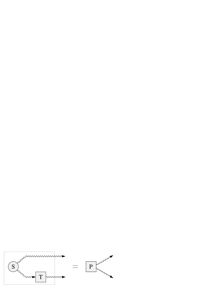
Figure 6.3: The duality scheme of Lemma 7: an arbitrary preparation P is uniquely represented as preparation S of a pure state and the application of a channel $T$ to half of the system.

Lemma 7

Let $\rho$ be a density operator on ${\cal H}\otimes{\cal K}$. Then there is a Hilbert space ${\cal H}^{\prime}$, a pure state $\sigma$ on ${\cal H}\otimes{\cal H}^{\prime}$, and a channel $T:{\cal B}({\cal K})\to{\cal B}({\cal H}^{\prime})$ such that

$$\rho=\sigma\circ({\rm id}_{\cal H}\otimes T)\;.$$ (6.9)

Moreover, the restriction of $\sigma$ to ${\cal H}^{\prime}$ can be chosen to be non-singular, and in this case the decomposition is unique in the sense that any other decomposition $\rho=\sigma^{\prime}\circ({\rm id}_{\cal H}\otimes T^{\prime})$ is of the form $\sigma^{\prime}=\sigma\circ R$ and $T^{\prime}=R^{-1}T$ with a unitarily implemented channel $R$.

It is clear that $\sigma$ must be the purification of $\rho$, restricted to the first factor. Thus we may set $\sigma=|\Psi\rangle\langle\Psi|$, with $\Psi=\sum_{k}\sqrt{r_{k}}\;e_{k}\otimes e^{\prime}_{k}$, where $r_{k}>0$ are the non-zero eigenvalues of the restriction of $\rho$ to the first system, and $e^{\prime}_{k}$ is a basis of ${\cal H}^{\prime}$. Note that the $e_{k}^{\prime}$ are indeed unique up to a unitary transformation, so we only have to show that for one choice of $e_{k}^{\prime}$ we get a unique $T$. From the equation $\rho=\sigma\circ({\rm id}_{\cal H}\otimes T)$ we can then read off the matrix elements of $T$:

$$\langle e^{\prime}_{k},\;T(|e_{\mu}\rangle\langle e_{\nu}|)\;e^{\prime}_{\ell}\rangle=r_{k}^{-1/2}r_{\ell}^{-1/2}\rho\bigl{(}|e_{k}\otimes e_{\mu}\rangle\langle e_{\ell}\otimes e_{\nu}|\;.$$ (6.10)

We have to show that $T$ as defined by this equation is completely positive whenever $\rho$ is positive. For fixed coefficients $r_{k}$ the map $\rho\mapsto T$ is obviously linear. Hence it suffices to prove complete positivity for $\rho=|\varphi\rangle\langle\varphi|$. But in that case $T=V^{*}AV$ with $\langle e_{\nu},\;Ve_{\ell}^{\prime}\rangle=r_{\ell}^{-1/2}\langle e_{\ell}\otimes e_{\nu},\varphi\rangle$, so $T$ is indeed completely positive. Normalization $T({\rm 1\mkern-5.4muI})={\rm 1\mkern-5.4muI}$ follows from the choice of $r_{k}$, and the Lemma is proved.

The main use of this Lemma is to translate results about entangled states to results about channels and conversely. For this it is necessary to have a translation table of properties. Some entries are easy: for example, $\rho$ is a product state iff $T$ is depolarizing in the sense that $T(A)={\mathop{\rm tr}\nolimits}(\rho_{2}A)$ for some density operator $\rho_{2}$, and $\rho$ is separable in the sense of Definition 2 iff $T$ is separable (see equation (6.5)).

6.4 Channel Capacity

In the definition of channel capacity we will have to use a criterion for the approximation of one channel by another. Since channels are maps between normed spaces, one obvious choice would be using the standard norm

$$\|S-T\|:=\sup\bigl{\{}\|S(A)-T(A)\|\;\mid\;\|A\|\leq 1\bigr{\}}\;.$$ (6.11)

However, as in the case of positivity there is a problem with this definition, when one considers tensor products: the norms $\|T\otimes{\rm id}_{n}\|$, with ${\rm id}_{n}$ the identity on ${\cal M}_{n}$, may increase with $n$. This introduces complications when one has to make estimates for parallel channels. Therefore we stabilize the norm with respect to tensoring with “innocent bystanders”, and introduce, for any linear map $T$ between C*-algebras

$$\|T\|_{\rm cb}:=\sup_{n}\|T\otimes{\rm id}_{n}\|\;,$$ (6.12)

called the norm of complete boundedness, or “cb-norm” for short. This name derives from the observation that on infinite dimensional C*-algebras the above supremum may be infinite even though each term in the supremum is finite. By definition, a completely bounded map is one with $\|T\|_{\rm cb}<\infty$. On a finite dimensional C*-algebra, every linear map is completely bounded: for maps into ${\cal M}_{d}$ we have $\|T\|_{\rm cb}\leq d\|T\|$. (As a general reference for these matters I recommend the book [20]). One might conclude from this that the whole distinction between these norms is irrelevant. However, since we will need estimates for large tensor products, every factor increasing with dimension can make a decisive difference. This is the reason for employing the cb-norm in the definition of channel capacity. It will turn out, however, that in the most important cases one has only to estimate differences to the identity, and $\|T-{\rm id}\|$ and $\|T-{\rm id}\|_{\rm cb}$ can be estimated in terms of each other with dimension-independent bounds.

The basis of the notion of channel capacity is the comparison between the given channel $T:{\cal A}_{2}\to{\cal A}_{1}$ and an “ideal” channel $S:{\cal B}_{1}\to{\cal B}_{2}$. The comparison is affected by suitable encoding and decoding transformations $E:{\cal A}_{1}\to{\cal B}_{1}$ and $D:{\cal B}_{2}\to{\cal A}_{2}$ so that the composed operator $ETD:{\cal B}_{2}\to{\cal B}_{1}$ is a map which can be compared directly with the ideal channel $S$. Of course, we are only interested in the comparison in the case of optimal encoding and decoding, i.e., in the quantity

$$\Delta(S,T)=\inf_{E,D}\|S-ETD\|_{\rm cb}\;,$$ (6.13)

where the infimum is over all channels (i.e., all unit preserving completely positive maps) $E$ and $D$ with appropriate domain and range. Since these data are at least implicitly given together with $S$ and $T$, there is no need to specify them in the notation. $S$ should be thought of as representing one word of the kind of message to be sent, whereas $T$ represents one invocation of the channel. Channel capacity is defined as the number of $S$-words per invocation of the channel $T$, which can be faithfully transmitted with suitable encoding and decoding for long messages. Here “messages of length $n$” are represented by the tensor power $S^{\otimes n}$, and “$m$ invocations of the channel $T$” are represented by the tensor power $T^{\otimes m}$.

Definition 8

Let $S$ and $T$ be channels. Then a number $c\geq 0$ is called an “achievable rate for $T$ with respect to $S$”, if for any sequences $n_{\alpha},m_{\alpha}$ of integers with $m_{\alpha}\to\infty$ and $\limsup_{\alpha}(n_{\alpha}/m_{\alpha})<c$ we have

$$\lim_{\alpha}\Delta\bigl{(}S^{\otimes n_{\alpha}},T^{\otimes m_{\alpha}}\bigr{)}=0\quad.$$

The supremum of all achievable rates is called the capacity of $T$ with respect to $S$, and is denoted by $C(S,T)$.

Note that by definition $0$ is an achievable rate (no integer sequences with asymptotically negative ratio exist), hence $C(S,T)\geq 0$. If all $c\geq 0$ are achievable, then of course we write $C(S,T)=\infty$. It may seem cumbersome to check all pairs of integer sequences with given upper ratio when testing $c$. However, due to some monotonicity of $\Delta$ it suffices to check only one sequence, provided it is not too sparse: if there is any pair of sequences $n_{\alpha},m_{\alpha}$ satisfying the conditions in the definition (including $\Delta\to 0$) plus the extra requirement that $(m_{\alpha}/m_{\alpha+1})\to 1$, then $c$ is achievable.

The ideal channel for systems with observable algebra ${\cal A}$ is by definition the identity map ${\rm id}_{\cal A}$ on ${\cal A}$. For typographical convenience we will abbreviate “${\rm id}_{\cal A}$” to “${\cal A}$”, whenever it appears as an argument of $\Delta$ or $C$. Using this notation, we will now summarize the capacities of ideal quantum and classical channels. Of course, these are basic data for the whole theory.

$$C({\cal M}_{k},{\cal C}_{n}) = 0\;,\quad\hbox{for $k\geq 2$}$$ (6.14)

$$C({\cal C}_{k},{\cal C}_{n}) = C({\cal M}_{k},{\cal M}_{n})=C({\cal M}_{k},{\cal C}_{n})=\frac{\log n}{\log k}\;.$$ (6.15)

Here the first equation is the capacity version of the No-Teleportation Theorem: It is impossible to transport any quantum information on a classical channel. The second line shows that for capacity purposes the ${\cal M}_{n}$ is indeed best compared with ${\cal C}_{n}$. In classical information theory one uses the 1 bit system ${\cal C}_{2}$ as the ideal reference channel. Similarly, we use the 1 qubit channel as the reference standard for quantum information , i.e., we define the classical capacity $C_{c}(T)$, and the quantum capacity $C_{q}(T)$, of an arbitrary channel by

$$C_{c}(T) = C({\cal C}_{2},T)$$ (6.16)

$$C_{q}(T) = C({\cal M}_{2},T)\;.$$ (6.17)

Combining the results (6.15) with the “triangle inequality”, or two step coding inequality

$$C(T_{1},T_{3})\geq C(T_{1},T_{2})C(T_{2},T_{3})$$ (6.18)

we see that this is really only a choice of units, i.e., for arbitrary channels $T$ we get $C({\cal M}_{n},T)=\frac{\log 2}{\log n}C({\cal M}_{2},T)$, and a similar equation for classical capacities. Note that the term “qubit” refers to the reference system ${\cal M}_{2}$, but it is not advisable to use it as a special unit for quantum information (rather than just “bit”): this would be like distinguishing the units “vertical meter” and “horizontal meter”, and create problems in every equation in which the two capacities are directly compared. The simplest relation of this kind is

$$C_{q}(T)\leq C_{c}(T)\;,$$ (6.19)

which follows by combining (6.18) with (6.15). Note that both definitions apply to arbitrary channels $T$, whether input and/or output are classical or quantum or hybrids. In order for a channel to have positive quantum capacity, it is necessary that both the input and the output are quantum systems. This is shown combining (6.14) with the bottleneck inequality

$$C(S,T_{1}T_{2})\leq\min\bigl{\{}C(S,T_{1}),C(S,T_{2})\bigr{\}}\;.$$ (6.20)

Another application of the bottleneck inequality is to separable channels. These are by definition the channels with a purely classical intermediate stage, i.e., $T=SR$ with ‘output of $S$’= ‘input of $R$’ a classical system. For such channels $C_{q}(T)=0$.

An important operation on channels is running two channels in parallel, represented mathematically by the tensor product. The relevant inequality is

$$C(S,T_{1}\otimes T_{2})\geq C(S,T_{1})+C(S,T_{2})$$ (6.21)

For the standard ideal channels, and when all systems involved are classical, we even have equality. However, it is one of the big open problems to decide under what general circumstances this is true.

Comparison with the classical definition

Since the definition of classical capacity $C_{c}(T)$ also applies to the purely classical situation, we have to verify that it is indeed equivalent to the standard definition in this case. To that end we have to evaluate the error quantity $\|T-{\rm id}\|_{\rm cb}$ for a classical to classical channel. As noted in a classical channel $T:{\cal C}(Y)\to{\cal C}(X)$ is given by a transition probability matrix $T(x\to y)$. Since the cb-norm coincides with the ordinary norm in the classical case, we get

$$\|{\rm id}-T\|_{\rm cb} = \|{{\rm id}-T}\|=\sup_{x,f}\Bigl{|}\sum_{y}\Bigl{(}\delta_{xy}-T(x\to y)\Bigr{)}f(y)\Bigr{|}$$

$$= 2\sup_{x}\bigl{(}1-T(x\to x)\bigr{)}\;$$

where the supremum is over all $f\in{\cal C}(Y)$ with $|f(y)|\leq 1$ and is attained where $f$ is just the sign of the parenthesis in the second line, and we used the normalization of transition probabilities. Hence, apart from an irrelevant factor two, $\|T-{\rm id}\|_{\rm cb}$ is just the maximal probability of error, i.e., the largest probability for sending $x$ and getting anything different. This is precisely the quantity, which is demanded to go to zero (after suitable coding and decoding) in Shannon’s classical definition of the channel capacity of discrete memoryless channels [5]. Hence the above definition agrees with the classical one.

When considering the classical capacity $C_{c}(T)$ of a quantum channel, it is natural to look at a coded channel $ETD$, as a channel in its own right. Since we consider transmission of classical information, this is a purely classical channel, and we can look at its classical capacity. Optimizing over coding and decoding, we get the quantity

$$C_{c,1}(T)=\sup_{ETD\ \rm classical}C_{c}(ETD)\;.$$ (6.22)

This is called the one-shot classical capacity, because it seems to involve only one invocation of the channel $T$. Of course, many uses of the channel are implicit in the capacity on the right hand side, but these are in some sense harmless. In fact, every coding and decoding scheme for comparing $(ETD)^{\otimes n}$ to an ideal classical channel is also a coding/decoding for $T^{\otimes n}$, but the codings/decodings arising in this way from coding $ETD$ are only those, in which the coded input states and measurements at the outputs are not entangled. If we allow entanglement over blocks of a large length $\ell$ we thus recover the full classical capacity:

$$C_{c,1}(T)\leq C_{c}(T)=\sup_{\ell}\ \frac{1}{\ell}\ C_{c,1}(T^{\otimes\ell})\;.$$ (6.23)

It is not clear, whether equality holds here. This is a fundamental question, which can be paraphrased as this: “Does entangled coding ever help for sending classical information over quantum channels?”. At the moment all partial results known to me seem to say that this is not the case.

Comparison with other error criteria

Coming now to the quantum capacity $C_{q}(T)$, we have relate our definition to more current ones. One version, first stated by Bennett is very similar to the one given above, but differs slightly in the error quantity, which is required to go to zero. Rather than $\|T-{\rm id}\|_{\rm cb}$, he considers the lowest fidelity of the channel, defined as

$${\cal F}(T)=\inf_{\psi}\langle\psi,T\bigl{(}|\psi\rangle\langle\psi|\bigr{)}\psi\rangle\;,$$ (6.24)

where the supremum is over all unit vectors. Hence achievable rates are those for which ${\cal F}(ET^{\otimes n_{\alpha}}D)\to 1$, where $E,D$ map to a system of $m_{\alpha}$ qubits, and these integer sequences satisfy the same constraints as above. This is definition is equivalent to ours, because the error estimates are equivalent. In fact, if we introduce the off-diagonal fidelity

$${\cal F}_{\%}(T)=\sup_{\phi,\psi}\Re\!e\langle\phi,T\bigl{(}|\phi\rangle\langle\psi|\bigr{)}\psi\rangle$$ (6.25)

for any channel $T:{\cal M}_{d}\to{\cal M}_{d}$ with $d<\infty$, we have the following system of estimates:

$$\|T-{\rm id}\| \leq \|T-{\rm id}\|_{\rm cb}\leq 4\sqrt{1-{\cal F}_{\%}(T)}\leq 4\sqrt{\|T-{\rm id}\|}$$ (6.26)

$$\|T-{\rm id}\| \leq 4\sqrt{1-{\cal F}(T)}\leq 4\sqrt{1-{\cal F}_{\%}(T)}\;,$$ (6.27)

which will be proved elsewhere. The main point is, though that the dimension does not appear in these estimates, so if one such quantity goes to zero, all others do, and we can build an equivalent capacity definition on any one of them.

Yet another definition of quantum capacity has been given in terms of entropy quantities [32], and was also shown to be equivalent [31].

6.5 Coding Theorems

The definition of channel capacity looks simple enough, but computing it on the basis of this definition is in general a very hard task: it involves an optimization over all coding and decoding channels in systems of asymptotically many tensor factors. Hence it is crucial to get simpler expressions, which can be computed in a much more direct way from the matrix elements of the given channel. Such results are called coding theorems, after the first theorem of this type, established by Shannon.

In order to state it we need some entropy quantities. The von Neumann entropy of a state with density matrix $\rho$ is defined as

$$S(\rho)=-{\mathop{\rm tr}\nolimits}\bigl{(}\rho\log\rho\bigr{)}\;,$$ (6.28)

where the function of $\rho$ is evaluated in the functional calculus, and $0\log 0$ is defined to be zero. The logarithm will be chosen to be base 2, so the unit for entropies is “bit”. The relative entropy of a state $\rho$ with respect to another, $\sigma$, is defined by

$$S(\rho,\sigma)={\mathop{\rm tr}\nolimits}\bigl{(}\rho(\log\rho-\log\sigma)\bigr{)};$$ (6.29)

Both quantities are positive, and may be infinite on an infinite dimensional space. The von Neumann entropy is concave, whereas the relative entropy is convex jointly in both arguments. For more precise definitions, and many further results, I recommend the book of Petz and Ohya [21].

The strongest coding theorem for quantum channels known so far is the following expression for the one-shot classical capacity, proved by Holevo [23]

$$C_{c,1}(T)=\max\left[S\Bigl{(}\sum_{i}p_{i}T_{*}[\rho_{i}]\Bigr{)}-\sum_{i}p_{i}S(T_{*}[\rho_{i}])\right]$$ (6.30)

Whether or not this is equal to the classical capacity depends on whether the conjectured equality in equation (6.23) holds or not. In any case, it is known to hold for channels with classical input, so Holevo’s coding theorem is a genuine extension of Shannon’s.

For the quantum capacity no coding theorem has been proved yet. However, there is a fairly good candidate for the right hand side, related to a quantity called “coherent information” [24]. The formula is written most compactly by relating it to an entanglement quantity via Lemma 7. For any bipartite state $\rho$ with restriction $\rho^{B}$ to the second factor, let

$$E_{S}(\rho)=S(\rho^{B})-S(\rho)\;.$$ (6.31)

This is an entanglement measure of sorts, because it is large when $S(\rho)$ is small, e.g., when $\rho$ is pure, and $\rho^{B}$ is very mixed, e.g., when $\rho$ is maximally entangled. It can be negative, though (see [25] for a discussion). Then we set

$$C_{S,1}(T)=\sup_{\sigma}\;E_{S}(\sigma\circ({\rm id}\otimes T))\;,$$ (6.32)

where the supremum is over all bipartite pure states $\sigma$. Note that any measure of entanglement can be turned into a capacity-like expression by this procedure. Since this quantity is known not to be additive [26], the candidate for the right hand side of the quantum coding theorem is

$$C_{S}(T)=\sup_{\ell}\ \frac{1}{\ell}\ C_{S,1}(T^{\otimes\ell})\;,$$ (6.33)

in analogy to (6.23). So far there are some good heuristic arguments [27, 28] in that direction, but a full proof remains one of the main challenges in the field.

An interesting upper bound on $C_{q}(T)$ can be written in terms of the transpose operation $\Theta$ on the output system [16]: one has

$$C_{q}(T)\leq\log_{2}\|\Theta T\|_{\rm cb}\;.$$ (6.34)

Hence if $\Theta T$ happens to be completely positive (as for any channel with an intermediate classical state) this map is a channel, hence has cb-norm $1$, and $C_{q}(T)=0$. This criterion can also be used to show that whenever there is sufficiently high noise in a channel, it will have quantum capacity zero.

6.6 Teleportation and Dense Coding Schemes

In this section we will show that entanglement assisted teleportation and dense coding as described in Sections 4.3 and 4.4 really work.

Rather than going through the now standard derivations in the basic qubit examples, we will use the structure assembled so far to reverse the question, i.e., we try to find the most general setup in which teleportation and dense coding work without errors. This will some give additional insights, and possibly some welcome flexibility when it comes to realizing these processes for larger than qubit systems. The task as stated is somewhat beyond the scope of this paper, mainly because there are so many ways to waste resources, which do not necessarily have a compact characterization. So in order to get a readable result, we only look at the “tight case” [29], in which resources are used in a sense optimally. By this we mean that all Hilbert spaces involved have the same finite but arbitrary dimension $d$ (so we can take them all equal to ${\cal H}={\mathbb{C}}^{d}$), and the classical channel distinguishes exactly $|X|=d^{2}$ signals.

For both teleportation and dense coding the beginning of each transmission is to distribute the parts of an entangled state $\omega$ between sender Alice and receiver Bob. Only then Alice is given the message she is supposed to send, which is a quantum state in the case of teleportation and a classical value in case of dense coding. She codes this in a suitable way, and Bob reconstructs the original message by evaluating Alice’s signal jointly with his entangled subsystem.

For dense coding, assume that $x\in X$ is the message given to Alice. She encodes it by transforming her entangled system by a channel $T_{x}$, and sending the resulting quantum system to Bob, who measures an observable $F$ jointly on Alice’s particle and his. The probability for getting $y$ as a result is then ${\mathop{\rm tr}\nolimits}\bigl{(}\omega(T_{x}\otimes{\rm id})(F_{y})\bigr{)}$, where the “$\otimes{\rm id}$” expresses the fact that no transformation is done to Bob’s particle while Alice applies $T_{x}$ to hers. If everything works correctly, this expression has to be $1$ for $x=y$, and $0$ otherwise:

$${\mathop{\rm tr}\nolimits}\bigl{(}\omega(T_{x}\otimes{\rm id})(F_{y})\bigr{)}=\delta_{xy}\;.$$ (6.35)

Let us take a similar look at teleportation. Here three quantum systems are involved: the entangled pair in state $\omega$, and the input system given to Alice, in state $\rho$. Thus the overall initial state is $\rho\otimes\omega$. Alice measures an observable $F$ on the first two factors, obtaining a result $x$ sent to Bob. Bob applies a transformation $T_{x}$ to his particle, and makes a final measurement of an observable $A$ of his choice. Thus the probability for Alice measuring $x$ and for Bob getting a result “yes” on $A$, is ${\mathop{\rm tr}\nolimits}(\rho\otimes\omega)(F_{x}\otimes T_{x}(A))$. Note that the tensor symbols in this equation refer to different splittings of the system ($1\otimes 23$ and $12\otimes 3$, respectively). Teleportation is successful, if the overall probability for getting $A$, computed by summing over all possibilities $x$, is the same as for an ideal channel, i.e.,

$$\sum_{x\in X}{\mathop{\rm tr}\nolimits}(\rho\otimes\omega)(F_{x}\otimes T_{x}(A))={\mathop{\rm tr}\nolimits}(\rho A)\;.$$ (6.36)

Surprisingly, in the tight case one gets exactly the same conditions on $\omega,T_{x},F_{x}$ for teleportation and dense coding, i.e., a dense coding scheme can be turned into a teleportation scheme simply by letting Bob and Alice swap their equipment. However, this symmetry depends crucially on the tightness condition, because teleportation schemes with $|X|>d^{2}$ signals are trivial to get, but $|X|>d^{2}$ is impossible for dense coding. Conversely, dense coding through a $d^{\prime}>d$ dimensional channel is trivial to get, while teleportation of states with $d^{\prime}>d$ dimensions (with the same $X$) is impossible.

Let us now give a heuristic sketch of the arguments leading to the necessary and sufficient conditions on for equations (6.36) and (6.35) to hold. For full proofs we refer to [29]. A crucial ingredient for the analysis of the teleportation equation is the “No measurement without perturbation” principle from Lemma 6: the left hand side of (6.36) is indeed such a decomposition, so each term must be equal to $\lambda_{x}{\mathop{\rm tr}\nolimits}(\rho A)$ for all $\rho,A$. But we can carry this even further: suppose we decompose $\omega,F_{x}$, or $T_{x}$ into a sum of (completely) positive terms. Then each term in the resulting sum must also be proportional to ${\mathop{\rm tr}\nolimits}(\rho A)$. Hence any components of $\omega,T_{x}$ and $F_{x}$ satisfy a teleportation equation as well (up to normalization). Similarly, the vanishing of the dense coding equation for $x\neq y$ carries over to every positive summand in $\omega,T_{x}$, or $F_{x}$. Hence it is plausible that we must first analyze the case where all $\omega,F_{x},T_{x}$ are “pure”, i.e., have no non-trivial decompositions as sums of (completely) positive terms:

$$\omega = |\Omega\rangle\langle\Omega|$$ (6.37)

$$F_{x} = |\Phi_{x}\rangle\langle\Phi_{x}|$$ (6.38)

$$T_{x}(A) = U_{x}^{*}AU_{x}\;.$$ (6.39)

The further analysis will show that in the pure case any two of these elements determine the third via the teleportation or the dense coding equation, so that in fact all components of $\omega$ (resp. $T_{x}$ or $F_{x}$) have to be proportional. Hence each of these has to be pure in the first place. For the present discussion, let us just assume purity in the form (6.37,…,6.39) from now on. Note that normalization requires that each $U_{x}$ is unitary.

The second normalization condition, $\sum_{x}|\Phi_{x}\rangle\langle\Phi_{x}|=\sum_{x}F_{x}={\rm 1\mkern-5.4muI}$ has an interesting consequence in conjunction with the tightness condition: the vectors $\Phi_{x}$ live in a $d^{2}$-dimensional space, and there are exactly $d^{2}$ of them. This implies that they are orthogonal: Since each vector $\Phi_{x}$ satisfies $\|\Phi_{x}\|\leq 1$, and $d={\mathop{\rm tr}\nolimits}({\rm 1\mkern-5.4muI})=\sum_{x}\|\Phi_{x}\|^{2}$, we must have $\|\Phi_{x}\|=1$ for all $x$. Hence in the sum $1=\sum_{x}\langle\Phi_{y},F_{x}\Phi_{y}\rangle$ the term $y=x$ is equal to $1$, and hence the others must be be zero.

Now consider the term with index $x$ in the teleportation equation and set $\rho=|\phi^{\prime}\rangle\langle\phi|$ and $A=|\psi\rangle\langle\psi^{\prime}|$. Then the trace splits into two scalar products, in which the variables ${\phi},{\phi^{\prime}},{\psi},{\psi^{\prime}}$ can be chosen independently, which leads to an equation of the form

$$\langle\phi\otimes\Omega,\Phi_{x}\otimes(U_{x}^{*}\psi)\rangle=\lambda_{x}\langle\phi,\psi\rangle\;,$$ (6.40)

for all $\phi,\psi$, and coefficients which must satisfy $\sum_{x}|\lambda_{x}|^{2}=1$. Note how in this equation a scalar product between the vectors in the first and third tensor factor is generated. This type of equation, which is clearly the core of the teleportation process may be solved in general:

Lemma 9

Let ${\cal H},{\cal K}$ be finite dimensional Hilbert spaces, and let $\Omega_{1}\in{\cal K}\otimes{\cal H}$ and $\Omega_{2}\in{\cal H}\otimes{\cal K}$ be unit vectors such that, for all $\phi,\psi\in{\cal H}$,

$$\langle\phi\otimes\Omega_{1},\Omega_{2}\otimes\psi\rangle=\lambda\langle\phi,\psi\rangle\;.$$ (6.41)

Then $|\lambda|\leq 1/\dim{\cal H}$ with equality iff $\Omega_{1}$ and $\Omega_{2}$ are maximally entangled and equal up to the exchange of the tensor factors ${\cal H}$ and ${\cal K}$.

For the proof consider the Schmidt decomposition $\Omega_{1}=\sum_{k}\sqrt{w_{k}}f_{k}\otimes e_{k}$, and insert $\phi=e_{n}$, $\psi=e_{m}$ into equation (6.41) to find the matrix elements of $\Omega_{2}$:

$$\langle e_{n}\otimes f_{m},\Omega_{2}\rangle=\lambda\;w_{m}^{-1/2}\ \delta_{nm}\;.$$

Clearly, $\|\Omega_{2}\|^{2}=|\lambda|^{2}\sum_{m}w_{m}^{-1}$. This sum takes its smallest value under the constraint $\sum_{m}w_{m}=\|\Omega_{1}\|^{2}=1$ only at the point where all $w_{m}$ are equal. This proves the Lemma.

We apply it to $\Omega_{1}=({\rm 1\mkern-5.4muI}\otimes U_{x})\Omega$, and $\Omega=\Phi_{x}$. Then $\sum_{x}|\lambda_{x}|^{2}\leq d^{2}d^{-2}=1$, with equality only if all the vectors involved are maximally entangled and pairwise equal up to an exchange of factors:

$$\Phi_{x}=(U_{x}\otimes{\rm 1\mkern-5.4muI})\Omega\;,$$ (6.42)

where we take $\Omega=d^{-1/2}\sum_{k}e_{k}\otimes e_{k}$ by an appropriate choice of bases. If $\Omega$ is maximally entangled, equation (6.42) sets up a one-to-one correspondence between unitary operators $U_{x}$ or the vectors $\Phi_{x}$ as independent elements in the construction. The $\Phi_{x}$ have to be an orthonormal basis of maximally entangled vectors, and there are no further constraints. In terms of the $U_{x}$ the orthogonality of the $\Phi_{x}$ translates in the orthogonality with respect to the Hilbert-Schmidt scalar product:

$${\mathop{\rm tr}\nolimits}(U_{x}^{*}U_{y})=d\;\delta_{xy}\;.$$ (6.43)

Again, there are no further constraints, so any collection of $d^{2}$ unitaries satisfying these equations leads to a teleportation scheme.

For dense coding case we get the same result, although along other routes. Equation (6.42) follows easily by writing the teleportation equation as $|\langle\Omega,(U_{x}^{*}\otimes{\rm 1\mkern-5.4muI})\Phi_{x}\rangle|^{2}=\delta_{xy}$. The problem is to show that $\Omega$ has to be maximally entangled. Using the reduced density operator $\omega_{1}$ of $\omega$, this becomes

$${\mathop{\rm tr}\nolimits}(\omega_{1}U_{x}^{*}U_{y})=\langle\Omega,(U_{x}^{*}U_{y}\otimes{\rm 1\mkern-5.4muI})\Omega\rangle=\langle\Phi_{x},\Phi_{y}\rangle=\delta_{xy}\;.$$ (6.44)

We claim that this equation, for a positive operator $\omega_{1}$, and $d^{2}$ unitaries $U_{x}$, implies that $\omega_{1}=d^{-1}{\rm 1\mkern-5.4muI}$. To see this, expand the operator $A=|\phi\rangle\langle e_{k}|\omega_{1}^{-1}$ in the basis $U_{x}$ according to the formula $A=\sum_{x}U_{x}{\mathop{\rm tr}\nolimits}(U_{x}^{*}A\omega_{1})$:

$$\sum_{x}\langle e_{k},U_{x}^{*}\phi\rangle\ U_{x}=|\phi\rangle\langle e_{k}|\omega_{1}^{-1}\;.$$

Taking the matrix element $\langle\phi|\cdot|e_{k}\rangle$ of this equation, and summing over $k$, we find

$$\sum_{x,k}\langle e_{k},U_{x}^{*}\phi\rangle\ \langle\phi,U_{x}e_{k}\rangle=\sum_{x}{\mathop{\rm tr}\nolimits}(U_{x}^{*}|\phi\rangle\langle\phi|U_{x})=d^{2}\|\phi\|^{2}=\|\phi\|^{2}\;{\mathop{\rm tr}\nolimits}(\omega_{1}^{-1})\;.$$

Hence ${\mathop{\rm tr}\nolimits}(\omega_{1}^{-1})=d^{2}=\sum_{k}r_{k}^{-1}$, where $r_{k}$ are the eigenvalues of $\omega_{1}$. Using again that the smallest value of this sum under the constraint $\sum_{k}r_{k}=1$ is attained only for constant $r_{k}$, we find $\omega_{1}=d^{-1}{\rm 1\mkern-5.4muI}$, and $\Omega$ is indeed maximally entangled.

To summarize, we have the following Theorem (again, for a detailed proof see [29]):

Theorem 10

Given either a teleportation scheme or a dense coding scheme, which is tight in the sense that all Hilbert spaces are $d$-dimensional, and $|X|=d^{2}$ classical signals are distinguished. Then

• $\omega=|\Omega\rangle\langle\Omega|$ is pure and maximally entangled,

• $F_{x}=|\Phi_{x}\rangle\langle\Phi_{x}|$, where the $\Phi_{x}$ form an orthonormal basis of maximally entangled vectors,

• $T_{x}(A)=U_{x}^{*}AU_{x}$, where the $U_{x}$ are unitary and orthonormal in the sense that ${\mathop{\rm tr}\nolimits}(U_{x}^{*}U_{y})=d\;\delta_{xy}$, and

• these objects are connected by the equation $\Phi_{x}=(U_{x}\otimes{\rm 1\mkern-5.4muI})\Omega$.

Given either the $\Phi_{x}$ or the $U_{x}$ with the appropriate orthogonality properties, and a maximally entangled vector $\Omega$, the above conditions determine a dense coding and a teleportation scheme.

In particular, we have shown that a teleportation scheme becomes a dense coding scheme, and conversely, when Alice and Bob swap their equipment. However, this is only true in the tight case: for a larger quantum channel dense coding becomes easier but teleporting becomes more demanding. Similarly, teleportation becomes easier with more allowed classical information exchange, whereas dense coding of more than $d^{2}$ signals is impossible.

In order to construct a scheme, it is best to start from the equation ${\mathop{\rm tr}\nolimits}(U_{x}^{*}U_{y})=d\;\delta_{xy}$, i.e., to look for orthonormal bases in the space of operators consisting of unitaries. For $d=2$ the solution is essentially unique: $U_{1},\ldots,U_{4}$ are the identity and the three Pauli matrices, which leads to the standard examples of. Group theory helps to construct examples of such bases for any dimension $d$, but this construction by no means exhausts the possibilities. A fairly general construction is given in [29]. It requires two combinatorial structures known from classical design theory [37]: a Latin square of order $d$, i.e., a matrix in which each row and column is a permutation of $(1,...,d)$, and $d$ Hadamard matrices, i.e., unitary $d\times d$-matrices, in which each entry has modulus $d^{-1/2}$. For neither Latin squares nor Hadamard matrices an exhaustive construction exists, so these are rich fields for hunting and gathering new examples, or even infinite families of examples. Certainly this connection suggests that a full classification or exhaustive construction of teleportation and dense coding schemes cannot be expected. However, it may still be a good project to look for schemes with additional desirable features.

Bibliography

- [1] L. Grover: “Quantum mechanics helps in searching for a needle in a haystack,”, Phys. Rev. Lett. 79 (1997) 325 (quant-ph/9706033).
- [2] A.R. Calderbank and P.W. Shor: “Good Quantum Error-Correcting Codes Exist”, Phys. Rev. A 54 (1996) 1098-1106 (quant-ph/9512032)
- [3] R. Laflamme, C. Miquel, J.P. Paz, and W.H. Zurek: “Perfect Quantum Error Correcting Code”, Phys.Rev.Lett. 77 (1996) 198-201 (quant-ph/9602019)
- [4] W.K. Wootters, W.H. Zurek: “A single quantum cannot be cloned”, Nature 299 (1982) 802–803
- [5] C.E. Shannon: “A mathematical theory of communication”, Bell System Technical Journal 27 (1948) 379-423 and 623-656
- [6] J.F. Clauser and A. Shimony: “Bell’s theorem: Experimental tests and implications”, Rep. Prog. Phys., 41 (1978) 1881-1927.
- [7] R. Derka, V. Bužek, A.K. Ekert “Universal algorithm for optimal estimation of quantum states from finite ensembles”, Phys.Rev.Lett. 80 (1998)1571 (quant-ph/9707028)
- [8] N. Gisin, S. Massar: “Optimal quantum cloning machines”, Phys.Rev.Lett. 79 (1997) 2153–2156 (quant-ph/9705046)
- [9] M. Keyl, R.F. Werner: “Optimal cloning of pure states, judging single clones” J.Math.Phys.40 (1999) 3283-3299 (quant-ph/9807010)
- [10] V. Bužek, M. Hillery, and R.F. Werner: “Optimal manipulations with qubits: universal NOT gate” Phys.Rev. A 60 (1999) R2626-R2629 (quant-ph/9901053)
- [11] A. Aspect, P. Grangier and G. Roger: “Experimental tests of realistic local theories via Bell’s Theorem”, Phys.Rev.Lett 47 (1981) 460–463
- [12] C.H. Bennett, G. Brassard, C. Crepeau , R. Jozsa, A. Peres, and W.K. Wootters, “Teleporting an unknown quantum state via dual classical and Einstein-Podolsky-Rosen channels” Phys.Rev.Lett. 70 (1993) 1895–1899
- [13] J.I. Cirac, A.K. Ekert and C. Macchiavello: “Optimal purification of single qubits”, Phys. Rev. Lett. 82 (1999) 4344-4347 (quant-ph/9812075).
- [14] M. Keyl, R.F. Werner: “The rate of optimal purification procedures”, quant-ph/9910124, to appear in Ann. Henri Poincaré
- [15] C.H. Bennett, S.J. Wiesner, “Communication via one- and two-particle operators on Einstein-Podolsky-Rosen states”, Phys.Rev.Lett. 69(1992)2881–2884
- [16] A.S. Holevo and R.F.Werner: “Evaluating capacities of Bosonic Gaussian channels”, quant-ph/9912067, to appear in Phys.Rev. A
- [17] O. Bratteli and D. W. Robinson: Operator algebras and quantum statistical mechanics, vol. I (Springer 1979)
- [18] J. von Neumann: Mathematical foundations of quantum mechanics, (Princeton UP 1955)
- [19] K. Kraus: States, effects, and operations, Lecture Notes in Physics, Vol. 190, (Springer-Verlag, Berlin 1983)
- [20] V.I. Paulsen, Completely bounded maps and dilations, Longman Scientific and Technical 1986
- [21] M. Ohya and D. Petz: Quantum entropy and its use, (Springer 1993)
- [22] E.B. Davies, Quantum theory of open systems, (Academic Press, 1976)
- [23] A.S. Holevo, “Coding theorems for Quantum Channels,” Tamagawa University Research Review, No.4, 1998. (quant-ph/9809023).
- [24] H. Barnum, M.A. Nielsen, and B. Schumacher: “Information transmission through noisy quantum channels,” Phys. Rev. A A57 (1998) 4153-4175 (quant-ph/9702049).
- [25] N.J. Cerf, C. Adami: “Negative entropy and information in quantum mechanics,” Phys. Rev. Lett. 79 (1997) 5194 (quant-ph/9512022).
- [26] D.P. DiVincenzo, P.W. Shor, J.A. Smolin, “Quantum-channel capacity of very noisy channels,” Phys. Rev. A, 57, (1998) 830-839 (quant-ph/9706061).
- [27] S. Lloyd: “The capacity of the noisy quantum channel,” Phys. Rev. A, 56 (1997) 1613.
- [28] M. Horodecki, P. Horodecki, R. Horodecki: “Unified approach to quantum capacities: towards quantum noisy coding theorem,” Phys. Rev. Lett. 85, 433 (2000) (quant-ph/0003040)
- [29] R.F. Werner: “All Teleportation and Dense Coding Schemes”, quant-ph/0003070
- [30] W.F. Stinespring: “Positive functions on C*-algebras”, Proc.Amer.Math.Soc. 6 (1955) 211–216
- [31] H. Barnum, E. Knill, and M.A. Nielsen: “On quantum fidelities and channel capacities”, IEEE Transactions on Information Theory 46, 1317-1329, 2000. (quant-ph/9809010)
- [32] B.W. Schumacher: “Sending entanglement through noisy quantum channels”, Phys.Rev. A 54 (1996) 2614
- [33] P. Shor: “Polynomial-time algorithms for prime factorization and discrete logarithms on a quantum computer,” SIAM J. Computing 26 (1997) 1484 (quant-ph/9508027).
- [34] S.J. Summers and R.F. Werner: “Maximal violation of Bell’s inequality is generic in quantum field theory”, Commun. Math. Phys. 110 (1987) 247-259
- [35] H. Halvorson and R. Clifton: “Generic Bell correlation between arbitrary local algebras in quantum field theory”, J.Math.Phys. 41 (2000) 1711-1717
- [36] W. Arveson: “Subalgebras of C*-algebras”, Acta math. 123 (1969) 141 - 224
- [37] T. Beth, D. Jungnickel, H. Lenz: Design Theory, 2nd edition, Encyclopedia of Mathematics and Its Applications , Vols. 69 and 78, (Cambridge Univ Press 2000)