New Tests of Macroscopic Local Realism using Continuous Variable Measurements

Abstract

We show that quantum mechanics predicts an Einstein-Podolsky-Rosen paradox (EPR), and also a contradiction with local hidden variable theories, for photon number measurements which have limited resolving power, to the point of imposing an uncertainty in the photon number result which is macroscopic in absolute terms. We show how this can be interpreted as a failure of a new, very strong premise, called macroscopic local realism. We link this premise to the Schrodinger-cat paradox. Our proposed experiments ensure all fields incident on each measurement apparatus are macroscopic. We show that an alternative measurement scheme corresponds to balanced homodyne detection of quadrature phase amplitudes. The implication is that where either EPR correlations or failure of local realism is predicted for quadrature phase amplitude measurements, one can potentially perform a modified experiment which would lead to conclusions about the much stronger premise of macroscopic local realism.

I Introduction

In 1935 Einstein, Podolsky and Rosen [1] (EPR) formulated an argument, now experimentally realised [2], in an attempt to show that quantum mechanics is an incomplete theory. The EPR argument is based on the premise of local realism. Bell [3] in 1966 showed that the premise of local realism (local hidden variable theories) was incompatible quantum mechanics. “Local realism” has now been essentially disproved by experiments [4] based on Bell’s theorem or those of Greenberger, Horne and Zeilinger (GHZ) [3].

To date the EPR and Bell theorems and experimental efforts primarily focus on measurements intrinsically microscopic, in that one requires to clearly distinguish between results (eigenvalues of the appropriate quantum operator) which are microscopically distinct. (An exception to this is the work of Peres [18].) Previous results [5] have indicated failure of local realism for macroscopic systems, but the violations are still apparently only indicated where measurements must resolve microscopically different results, such as adjacent photon number or spin values. It is not clear whether one is testing a premise different to that tested in the microscopic experiments.

We propose a strategy for testing local realism at a macroscopic level, in the sense emphasised by Schrodinger [6, 7] in his famous “cat” paradox and also by Leggett and Garg [8], where one considers macroscopically distinct outcomes. We define in section 2 the premise of “macroscopic local realism” [9], in such a way that it relates to the Schrodinger-cat example of macroscopically distinct states.

In section 3 we present an EPR argument based on the validity of “macroscopic local realism”, which has not yet been questioned. We suggest that modifications to an experiment already performed by Ou et al [2] would realise this macroscopic EPR argument and would leave no logical alternative except to deny the validity of macroscopic local realism or else to accept the incompleteness of quantum mechanics, in the sense proposed by EPR.

In section 4 we present a quantum state which allows a violation of a Bell-inequality even where all uncertainties in measurements are macroscopic, and show how this implies a predicted failure of macroscopic local realism.

II Definition of Macroscopic Local Realism

In 1935 Einstein, Podolsky and Rosen [1] defined “local realism”. “Realism” implies that if one can predict with certainty the result of a measurement of a physical quantity at $A$, without disturbing the system $A$, then the results of the measurement were predetermined. One has an “element of reality” corresponding to this physical quantity. The element of reality is a variable which assumes one of a set of values which are the predicted results of the measurement. This value gives the result of the measurement, should it be performed. Locality states that events at $A$ cannot, instantaneously, disturb a second system at $B$ spatially separated from $A$. Taken together “local realism” implies that, if one can predict the result of a measurement of a physical quantity at $A$, by making a simultaneous measurement at $B$, then the result of the measurement at $A$ is described by an element of reality.

EPR assumed quantum mechanics to be correct in predicting the existence of two spatially separated particles with correlated positions, and also correlated momenta. The key quantity in establishing the EPR argument is the precision (call the associated error $\Delta)$ to which the result of the potential position measurement at $A$ can be inferred by the measurement at $B$. This specifies an associated indeterminacy (error $\Delta)$ in the “element of reality” $x$. In the original EPR gedanken example, $\Delta$ is zero. “Local realism” establishes two “elements of reality”, $x$ and $p$ which simultaneously exist to give precisely the result of a potential position or momentum measurement, respectively. No description of this nature exists within quantum mechanics, since any quantum wavefunction gives an indeterminacy $\Delta x$ and $\Delta p$ in position and momentum respectively, in accordance with the uncertainty relation $\Delta x\Delta p\geq\hbar/2$. In this way, the EPR argument, based on the validity of “local realism”, allows one to conclude that quantum mechanics is incomplete.

Macroscopic local realism [9] is defined as a premise stating the following. If one can predict the result of a measurement at $A$ by performing a simultaneous measurement on a spatially separated system $B$, then the result of the measurement at $A$ is predetermined but described by an element of reality which has an indeterminacy in each of its possible values, so that only values macroscopically different to those predicted are excluded.

Macroscopic local realism is based on a “macroscopic locality”, which states that measurements at a location $B$ cannot instantaneously induce macroscopic changes (for example the dead to alive state of a cat, or a change between macroscopically different photon numbers) in a second system $A$ spatially separated from $B$. Macroscopic local realism also incorporates a “macroscopic realism”, since it implies elements of reality with (up to) a macroscopic indeterminacy. Suppose our “Schrodinger’s cat [6]” is correlated with a second spatially separated system, for example a gun used to kill the cat. The strength of macroscopic local realism is understood when one realises that its rejection in this example means we cannot think of the cat as being either dead or alive, even though we can predict the dead or alive result of “measuring” the cat, without disturbing the cat, by measurement on the correlated spatially-separated second system.

III An EPR Argument based on Macroscopic Local Realism

We consider a new EPR situation, depicted in Figure 1, where uncertainties in “elements of reality” become macroscopic. The $\hat{a}_{\pm}$ and $\hat{b}_{\pm}$ are boson operators for four fields, described by the quantum state $|\psi\rangle$. Fields $\hat{a}_{\pm}$ and $\hat{b}_{\pm}$ propagate towards the spatially separated locations $A$ and $B$ respectively. We measure simultaneously at $A$ and $B$ the Schwinger spin operators

$$\hat{S}_{\theta}^{A} = \hat{S}_{x}^{A}\cos{\theta}+\hat{S}_{y}^{A}\sin{\theta}$$ (1)

$$= (\hat{a}_{+}^{\dagger}\hat{a}_{-}\exp(-i\theta)+\hat{a}_{+}\hat{a}_{-}^{\dagger}\exp(i\theta))/2$$ (2)

and

$$\hat{S}_{\phi}^{B} = \hat{S}_{x}^{B}\cos{\phi}+\hat{S}_{y}^{B}\sin{\phi}$$ (3)

$$= (\hat{b}_{+}^{\dagger}\hat{b}_{-}\exp(-i\phi)+\hat{b}_{+}\hat{b}_{-}^{\dagger}\exp(i\phi))/2$$ (4)

respectively, where $\hat{S}_{x}^{A}=(\hat{a}_{+}^{\dagger}\hat{a}_{-}+\hat{a}_{-}^{\dagger}\hat{a}_{+})/2,\hat{S}_{y}^{A}=(\hat{a}_{+}^{\dagger}\hat{a}_{-}-\hat{a}_{-}^{\dagger}\hat{a}_{+})/2i$ and $\hat{S}_{z}^{A}=(\hat{a}_{+}^{\dagger}\hat{a}_{+}-\hat{a}_{-}^{\dagger}\hat{a}_{-})/2$, and similarly for the modes at $B$.

We propose to measure, at $A$, $\hat{S}_{x}^{A}$ or $\hat{S}_{y}^{A}$, by selecting $\theta=0$ or $\theta=\pi/2$. At $B$ the measurement is either $S_{x}^{B}$ or $S_{y}^{B}$. In Figure 1 the measurement at $A$ is performed by first mixing $\hat{a}_{\pm}$ using phase shifts and beam splitters to give two new fields $\hat{a}_{-}^{{}^{\prime}}=(\hat{a}_{-}-\hat{a}_{+})/\sqrt{2}$ and $\hat{a}_{+}^{{}^{\prime}}=i(\hat{a}_{-}+\hat{a}_{+})/\sqrt{2}$. Similarly $\hat{b}_{\pm}$ are mixed to give outputs $\hat{b}_{\pm}^{{}^{\prime}}$. The fields $a_{+},b_{+}$ are coherent states of large amplitude. The mixing is incorporated so that both fields, $\hat{a}_{\pm}^{{}^{\prime}}$ say at $A$, incident on the measuring apparatus are macroscopic. The final measurements are made with the transformations (using polarisers or beam splitters with variable transmission) $c_{+}=\hat{a}_{+}^{{}^{\prime}}\cos{\theta/2}+\hat{a}_{-}^{{}^{\prime}}\sin{\theta/2}$ and $c_{-}=\hat{a}_{+}^{{}^{\prime}}\sin{\theta/2}-\hat{a}_{-}^{{}^{\prime}}\cos{\theta/2}$, at $A$, and $d_{+}=\hat{b}_{+}^{{}^{\prime}}\cos{\phi/2}+\hat{b}_{-}^{{}^{\prime}}\sin{\phi/2}$ and $d_{-}=\hat{b}_{+}^{{}^{\prime}}\sin{\phi/2}-\hat{b}_{-}^{{}^{\prime}}\cos{\phi/2}$, at $B$, followed by photodetection to give $\hat{S}_{\theta}^{A}=(\hat{c}_{+}^{\dagger}\hat{c}_{+}-\hat{c}_{-}^{\dagger}\hat{c}_{-})/2$ and $\hat{S}_{\phi}^{B}=(\hat{d}_{+}^{\dagger}\hat{d}_{+}-\hat{d}_{-}^{\dagger}\hat{d}_{-})/2$. The measurement is one of photon number, and we define $\hat{n}_{\theta}^{A}=2\hat{S}_{\theta}^{A}=\hat{c}_{+}^{\dagger}\hat{c}_{+}-\hat{c}_{-}^{\dagger}\hat{c}_{-}$ and $\hat{n}_{\phi}=2\hat{S}_{\phi}^{B}=\hat{d}_{+}^{\dagger}\hat{d}_{+}-\hat{d}_{-}^{\dagger}\hat{d}_{-}$.

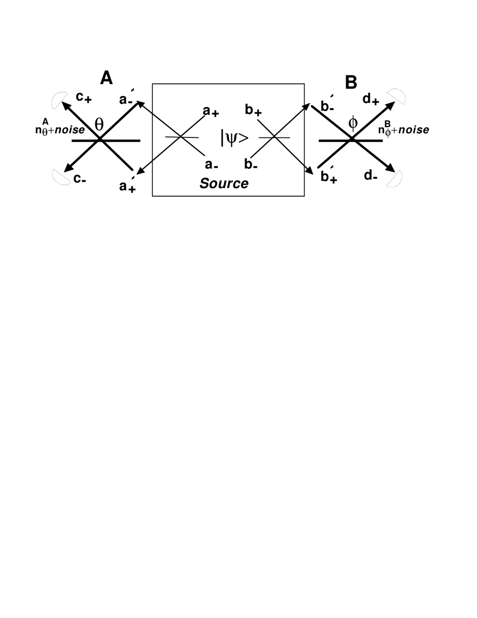
FIG. 1.: Schematic diagram of the experimental arrangement used to give the two different tests, described in sections 3 and 4, of macroscopic local realism. The $a_{+}$ and $b_{+}$ represent strong coherent states. For the macroscopic EPR experiment of section 3, the quantum state is chosen to ensure that the output fields $a_{-},b_{-}$ are EPR correlated with respect to quadrature phase amplitudes.

In Figure 2 we demonstrate how the measurement $\hat{S}_{\theta}^{A}$ can be performed using an alternative arrangement, by introducing a relative phase shift $\theta$ and mixing with a $50/50$ beam splitter to produce $\hat{c}_{\pm}^{{}^{\prime}}=\left(\hat{a}_{+}\pm\hat{a}_{-}\exp(-i\theta)\right)/\sqrt{2}$, followed by photodetection to give $\hat{S}_{\theta}^{A}=(\hat{c}_{+}^{{}^{\prime}\dagger}\hat{c}_{+}^{{}^{\prime}}-\hat{c}_{-}^{{}^{\prime}\dagger}\hat{c}_{-}^{{}^{\prime}})/2$. It is to be clarified below that this measurement scheme corresponds to homodyne measurement [10] (used  [2, 11] to detect subshot noise, or “squeezed”, radiation) of the quadrature phase amplitudes of $a_{-}$ and $b_{-}$.

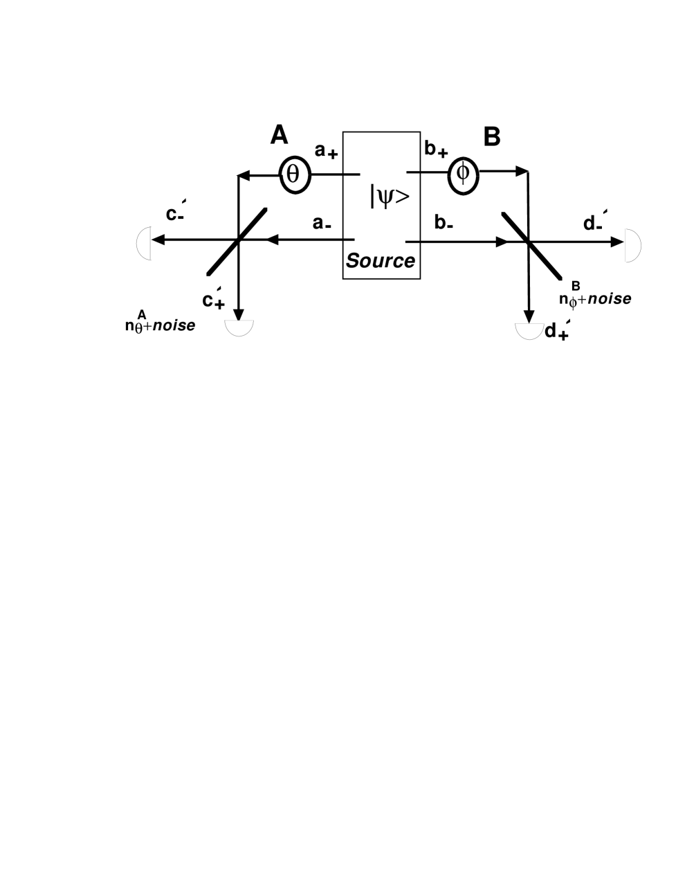
FIG. 2.: An alternative arrangement used to measure $n_{\theta}^{A}$ and $n_{\phi}^{B}$. Fields $a_{+},b_{+}$ are in coherent states of large amplitude $\alpha=\beta=E$. This measurement scheme corresponds to balanced homodyne detection of the quadrature phase amplitudes $\hat{X}_{\theta}^{A}$ and $\hat{X}_{\phi}^{B}$ (defined in section 4), the $a_{+},b_{+}$ being “local oscillator” fields.

For certain systems the results for $\hat{S}_{x}^{A}$ and $\hat{S}_{x}^{B}$, and also $\hat{S}_{y}^{A}$ and $\hat{S}_{y}^{B}$, are predicted by quantum mechanics to be correlated, so that elements of reality may be deduced for the physical quantities $S_{x}^{A}$ and $S_{y}^{A}$ respectively. We consider the relevant uncertainty relation for $\hat{S}_{x}^{A}$ and $\hat{S}_{y}^{A}$ [12].

$$\Delta\hat{S}_{x}^{A}\Delta\hat{S}_{y}^{A}\geq\left|\left\langle\hat{S}_{z}^{A}\right\rangle\right|/2=(\hat{a}_{+}^{\dagger}\hat{a}_{+}-\hat{a}_{-}^{\dagger}\hat{a}_{-})/4$$ (5)

Fields $\hat{a}_{+}$ and $\hat{b}_{+}$ are coherent states $|\alpha>$ and $|\beta>$ respectively with $\alpha=\beta=E$ real and large, so that $\hat{a}_{+}$ is replaced by c-number $E$ giving

$$\hat{S}_{x}^{A} = E\left(\hat{a}_{-}+\hat{a}_{-}^{\dagger}\right)/2=E\hat{X}_{0}^{A}/2$$ (6)

$$\hat{S}_{y}^{A} = E\left(\hat{a}_{-}-\hat{a}_{-}^{\dagger}\right)/2i=E\hat{X}_{\pi/2}^{A}/2$$ (7)

where $\hat{X}_{0}^{A}=\hat{a}_{-}+\hat{a}_{-}^{\dagger}$ and $\hat{X}_{\pi/2}^{A}=\left(\hat{a}_{-}-\hat{a}_{-}^{\dagger}\right)/i$ are quadrature phase amplitudes. We denote the indeterminacy in the “element of reality” $s_{x}^{A}$ by $\Delta_{x}$, and in the “element of reality” $s_{y}^{A}$ by $\Delta_{y}$. In order to exclude the possibility that the “elements of reality” cannot be described by a quantum wavefunction, it is sufficient to establish (here $\left\langle\hat{a}_{+}^{\dagger}\hat{a}_{+}\right\rangle>>\left\langle\hat{a}_{-}^{\dagger}\hat{a}_{-}\right\rangle$)

$$\Delta_{x}\Delta_{y}<\left|\left\langle\hat{S}_{z}^{A}\right\rangle\right|/2=E^{2}/4$$ (8)

The new feature of this EPR situation is the macroscopic nature of the minimum uncertainty product: $2\left|\left\langle\hat{S}_{z}^{A}\right\rangle\right|=E^{2}$ is a macroscopic (photon) number. The implication is that one need only use the premise of “macroscopic local realism”, rather than local realism in its entirety, to arrive at the conclusion that quantum mechanics is incomplete. With “macroscopic local realism”, one can only exclude the possibility of macroscopic changes to the system at $A$, as a result of measurements made at $B$. One can predict with some error ($\Delta_{1}$ and $\Delta_{2}$ say for the $x$ and $y$ spin components respectively) the result of the spin measurement at $A$. By macroscopic local realism, the spin is predetermined, but only to a precision which excludes values macroscopically different to those in the range predicted. The “element of reality” for the $x$ component of spin has a range of possible values, given by $\pm\Delta_{x}$ where $\Delta_{x}=\Delta_{1}+\delta$ and $\delta$ is microscopic or mesoscopic. The “element of reality” for the $y$ component has an indeterminacy $\pm\Delta_{y}$ where $\Delta_{y}=\Delta_{2}+\delta$. This can still be sufficient to imply the EPR criterion (5) since the uncertainty limit $E^{2}$ is a macroscopic number. We only require for example the differences $E/2-\Delta_{1}$ and $E/2-\Delta_{2}$ to be macroscopic numbers and we satisfy (5).

To meet the situation of a macroscopic EPR experiment, where macroscopic local realism is used in the EPR conclusions, one needs $\Delta_{1}\Delta_{2}<\left|\left\langle\hat{S}_{z}^{A}\right\rangle\right|/2=E^{2}/4$ satisfied, but where $2\left|\left\langle\hat{S}_{z}^{A}\right\rangle\right|=E^{2}$, and $2(E/2-\Delta_{1})$ and $2(E/2-\Delta_{2})$ are macroscopic photon numbers. From the point of view of performing an experiment which is convincingly macroscopic, the preference would be to satisfy these criteria where measurement errors, and therefore also $\Delta_{1}$ and $\Delta_{2}$, are also large (photon) numbers.

So far we have assumed the existence of the required correlations for the spin operators. Such correlated fields are predicted when $a_{-},b_{-}$ are fields with “EPR correlations” for quadrature phase amplitudes, and $a_{+},b_{+}$ are strong coherent fields. EPR correlations for quadrature phase amplitudes were defined in [12], and have received much interest as fields enabling quantum teleportation for continuous variables [13]. EPR fields may be generated by the parametric interaction $H=i\hbar\kappa\left(\hat{a}_{-}^{\dagger}\hat{b}_{-}^{\dagger}-\hat{a}_{-}\hat{b}_{-}\right)$, where here $\kappa$ represents the strength of nonlinear interaction. This two-mode squeezed light represents the logical choice for the quantum state $|\phi>$ in figure 1. (It is possible to generate the required EPR correlations from a single-mode squeezed state passed using a $50/50$ beam splitter [12, 13].)

Using the parametric example, we consider the quadrature phase amplitudes $\hat{X}_{0}^{A},\hat{X}_{\pi/2}^{A}$, and $\hat{X}_{0}^{B}$, $\hat{X}_{\pi/2}^{B}$ where $\hat{X}_{0}^{B}=b_{-}+b_{-}^{\dagger}$ and $\hat{X}_{\pi/2}^{B}=\left(\hat{b}_{-}-\hat{b}_{-}^{\dagger}\right)/i$. With vacuum inputs, the output solutions after a time $t$, for $\kappa t\rightarrow\infty$, satisfy $\hat{X}_{0}^{A}\left(t\right)=\hat{X}_{0}^{B}\left(t\right)$ and $\hat{X}_{\pi/2}^{A}\left(t\right)=-\hat{X}_{\pi/2}^{B}\left(t\right)$, indicating a maximum correlation^[13] between the results of measurements $\hat{X}_{0}^{A}\left(t\right)$ and $\hat{X}_{0}^{B}\left(t\right)$, and also $\hat{X}_{\pi/2}^{A}\left(t\right)$ and $\hat{X}_{\pi/2}^{B}\left(t\right).$ The $\hat{a}_{+},\hat{b}_{+}$ fields are coherent states $\left|\alpha\right\rangle$ and $\left|\beta\right\rangle$ of large intensity so that $\hat{S}_{x}^{A}=\alpha\hat{X}_{0}^{A}(t)/2$, $\hat{S}_{x}^{B}=\beta\hat{X}_{0}^{B}(t)/2$, $\hat{S}_{y}^{A}=\alpha\hat{X}_{\pi/2}^{A}(t)/2$ and $\hat{S}_{y}^{B}=\beta\hat{X}_{\pi/2}^{B}(t)/2$, and we have the required correlations. The reader is referred to articles [2, 12, 9] for information on the evaluation of $\Delta_{1}$ and $\Delta_{2}$.

The macroscopic EPR experiment performed with results in accordance with quantum mechanics would logically lead to the conclusion that: either macroscopic local realism is invalid; or that quantum mechanics is incomplete. EPR experiments have perhaps not yet been widely considered important in their own right, since previously they have been based on local realism, a premise dismissed by Bell inequality experiments. (Actually this is not quite correct, since detector inefficiencies have prevented a true violation of a Bell inequality. Proposed EPR quadrature experiments do not suffer this problem). In our macroscopic example this is not correct. The validity of macroscopic local realism has not been tested.

The macroscopic EPR experiment has been performed in a partly satisfactory way by Ou et al [2], with the arrangement of Figure 2. For a conclusive result the arrangement of Figure 1 is preferred. The experimental scheme of Ou et al suffers the disadvantage that fields $a_{-},b_{-}$ are microscopic. This is irrelevant in that the quantity measured, and to which the elements of reality relate, is not $\hat{X}_{\theta}^{A}$ but $\hat{S}_{\theta}^{A}$. Nevertheless, the microscopic nature of $\hat{a}_{-},\hat{b}_{-}$ incident on the measurement apparatus gives the impression of a microscopic experiment. The scheme of Figure 1 where both fields incident on the measurement apparatus are macroscopic is more transparent, making it clear that the “local oscillator” fields $a_{+},b_{+}$ form part of the system. It is also essential to ensure measurement events (the selection of $\theta$ or $\phi$) at $A$ and $B$ causally separated, as in delayed-choice Bell inequality experiments [4]. Since a wide variety of squeezing experiments have been performed, including squeezing in pulsed fields, an experimental realisation of the macroscopic EPR experiment would seem very feasible.

IV A Direct Test of Macroscopic Local Realism: Bell Inequalities based on Macroscopic Local Realism

We prove that for coarse measurements with macroscopic uncertainties, Bell inequalities can be derived using only the premise of macroscopic local realism [14]. Our proposed experiment is again depicted in Figure 1,, except that the quantum state $|\phi>$ will be chosen differently. The parametric interaction used as a source for EPR correlations in the Ou et al experiment is not directly siutable for this experiment, as in this case a positive Wigner function exists. This positive Wigner function can act as a local hidden variable theory to describe the quantum predictions [3], and thus prevent a violation of a Bell inequality as we derive here. With an appropriate choice of quantum state then, we measure simultaneously.

We measure simultaneously at $A$ and $B$ the Schwinger operators $\hat{S}_{\theta}^{A}$ and $\hat{S}_{\phi}^{B}$. The result for the photon number differences $\hat{n}_{\theta}^{A}$ and $\hat{n}_{\phi}^{B}$ is of the form $n+noise$, where $n$ is the result in the absence of the noise. We introduce a random noise function (gaussian distribution of standard deviation $\sigma$) at each of $A$ and $B$, and define probabilities such as $P^{A}(noise\geq x)$, that the $noise$ at $A$ is greater than or equal to the value $x$.

The results of measurements are classified as $+1$ if the photon number difference is positive or zero, and $-1$ otherwise. We determine the following probability distributions: $P_{+}^{A}(\theta)$ for obtaining $+$ at $A$; $P_{+}^{B}(\phi)$ for obtaining $+$ at $B$; and $P_{++}^{AB}(\theta,\phi)$ the joint probability of $+$ at both $A$ and $B$.

We define the probability $P_{ij}^{0,AB}(\theta,\phi)$ for obtaining results $i$ and $j$ respectively upon joint measurement of $\hat{n}_{\theta}^{A}$ at $A$, and $\hat{n}_{\phi}^{B}$ at $B$, in the absence of the applied noise $\sigma$. With noise present, measured probabilities become

$$P_{++}^{AB}(\theta,\phi)=\sum_{i,j=-\infty}^{\infty}P_{ij}^{0,AB}(\theta,\phi)P^{A}(noise\geq-i)P^{B}(noise\geq-j)$$ (9)

Local realism as defined by Einstein-Podolsky-Rosen, Bell and Clauser-Horne [1] implies the well known expression.

$$P_{ij}^{0,AB}(\theta,\phi)=\int\rho(\lambda)\quad p_{i}^{A}(\theta,\lambda)p_{j}^{B}(\phi,\lambda)\quad d\lambda$$ (10)

Local realism implies a set of elements of reality, or hidden variables $\lambda$ (with probability distribution $\rho(\lambda)$), not specified by quantum theory. For our experiment, a precise prediction of $\hat{n}_{\theta}^{A}$ is not possible given a measurement at $B$, for any choice $\phi$ at $B$. The elements of reality then do not take on definite values and local realism is only sufficient to imply a probability $p_{i}^{A}(\theta,\lambda)$ for the result $i$ of the measurement $\hat{n}_{\theta}^{A}$, for a given $\lambda$. The independence of $p_{i}^{A}(\theta,\lambda)$ on $\phi$ is based on the locality assumption.

With macroscopic local realism the locality condition is relaxed, but only up to the level of $M$ photons, where $M$ is not macroscopic, by maintaining that the measurement at $B$ cannot instantaneously change the result at $A$ by an amount exceeding $M$ photons. Where our predicted result at $A$ is $i^{{}^{\prime}}$ using local realism, macroscopic local realism allows the result to be $i=i^{{}^{\prime}}+m_{A}$ where $m_{A}$ can be any number not macroscopic. Importantly, while $i^{{}^{\prime}}$ is not dependent on the choice $\phi$ at $B$, the value $m_{A}$ which is not macroscopic can be. The macroscopic local realism assumption is that the conditional probability $p_{i}^{A}(\theta,\lambda)$ in equation (7) is expressible as the convolution:

$$p_{i}^{A}({\theta,\phi},\lambda)=\sum_{m_{A}=-M}^{+M}p_{m_{A}}^{A}(i^{{}^{\prime}},{\theta,\phi},\lambda)p_{i^{\prime}=i-m_{A}}^{A}(\theta,\lambda).$$ (11)

The original local probability $p_{i^{\prime}}^{A}(\theta,\lambda)$ can be convolved with a microscopic nonlocal probability function $p_{m_{A}}^{A}(i^{{}^{\prime}},{\theta,\phi},\lambda)$, the only restriction being that the nonlocal distribution does not provide macroscopic perturbations, so that the probability of getting a nonlocal change outside the range $m_{A}=-M,...,+M$ is zero. Equivalently we must have

$$\sum_{m_{A}=-M}^{M}p_{m_{A}}^{A}(i^{{}^{\prime}},{\theta,\phi},\lambda)=1.$$ (12)

We substitute the macroscopic locality assumption (8) into (7) to obtain the prediction for the measured probabilities (6). Recalling $i=i^{\prime}+m_{A}$, $j=j^{\prime}+m_{B}$ we change the $i$, $j$ summation to one over $i^{\prime}$, $j^{\prime}$ to get

$$P_{++}^{AB}(\theta,\phi) = \sum_{i^{\prime},j^{\prime}=-\infty}^{\infty}\int\rho(\lambda)p_{i^{\prime}}^{A}(\theta,\lambda)$$ (13)

$$\times \biggl{[}\sum_{m_{A}=-M}^{M}p_{m_{A}}^{A}(i^{{}^{\prime}},{\theta,\phi},\lambda)p_{j^{\prime}}^{B}(\phi,\lambda)P^{A}(noise\geq-(i^{\prime}+m_{A}))\biggr{]}\biggr{.}$$ (14)

$$\times \biggl{[}\sum_{m_{B}=-M}^{M}\biggl{.}p_{m_{B}}^{B}(j^{{}^{\prime}},{\phi,\theta},\lambda)P^{B}(noise\geq-(j^{\prime}+m_{B}))\biggr{]}d\lambda$$ (15)

We assume that the noise function $noise$ is slowly varying over the microscopic (or mesoscopic) range $-m_{A},..+m_{A}$ for which nonlocal perturbations are possible according to macroscopic local realism:

$$\sum_{m_{A}=-M}^{M}p_{m_{A}}^{A}(i^{{}^{\prime}},{\theta,\phi},\lambda)P^{A}(noise\geq-(i^{\prime}+m_{A}))$$ (16)

$$\approx P^{A}(noise\geq-i^{\prime})\sum_{m_{A}=-M}^{M}p_{m_{A}}^{A}(i^{{}^{\prime}},{\theta,\phi},\lambda).$$ (17)

This is only valid if $\sigma$ is macroscopic. Using (11), one simplifies to get the final form $P_{++}^{AB}(\theta,\phi)=\sum_{i^{\prime},j^{\prime}}\ \int\rho(\lambda)p_{i^{\prime}}^{A}(\theta,\lambda)p_{j^{\prime}}^{B}(\phi,\lambda)d\lambda\times P^{A}(noise\geq-i^{\prime})P^{B}(noise\geq-j^{\prime})$. This prediction of the hidden variable theory is now given in a (local) form like that of (7), from which Bell- Clauser-Horne inequalities [3] follow, for example:

$$S={{P_{++}^{AB}(\theta,\phi)-P_{++}^{AB}(\theta,\phi^{\prime})+P_{++}^{AB}(\theta^{\prime},\phi)+P_{++}^{AB}(\theta^{\prime},\phi^{\prime})}\over{P_{+}^{A}(\theta^{\prime})+P_{+}^{B}(\phi)}}\leq 1.$$ (18)

Violation of Bell inequalities (12) with macroscopic noise terms ($\sigma$ macroscopic) is evidence of a failure of macroscopic local realism. We propose a quantum state with this property ($I_{0}$ is a modified Bessel function, $r_{0}=1.1$).

$$|\psi\rangle=[I_{0}(2r_{0}^{2})]^{-1/2}|\alpha>_{a_{+}}|\beta>_{b_{+}}\left(\sum_{n=0}^{\infty}\frac{(r_{0}^{2})^{n}}{n!}|{n}>_{a_{-}}|{n}>_{b_{-}}\right).$$ (19)

$|\alpha>_{a_{+}}$ and $|\beta>_{b_{+}}$ are coherent states with $\alpha$, $\beta$ real and large. $|{n}>_{k}$ is a Fock state for field $k$. The fields $\hat{a}_{-}$ and $\hat{b}_{-}$ are microscopic and are generated in a pair-coherent state [15]. The quantum prediction for (13) is shown in Figure 3. Violations of the Bell inequality (12) in the absence of $noise$ are shown in curve (a). Violations are still possible (curve (b)) in the presence of increasingly larger absolute noise $\sigma$, simply by increasing $\alpha=\beta=E$. This violation of the Bell inequality (12) with macroscopic noise $\sigma$ implies the failure of macroscopic local realism.

FIG. 3.: (a) $S$ versus $\alpha=\beta$, for $\theta=0,\phi=-\pi/4,\theta^{\prime}=\pi/2,\phi^{\prime}=-3\pi/4$ for the quantum state (13) with no noise present. (b) Maximum noise $\sigma$ still giving a violation of the Bell inequality (12), versus $\alpha$.

The large $\alpha$,$\beta$ limit is crucial in determining whether the violation of macroscopic local realism will occur. We see from (1) and (2) that (letting $\alpha=\beta=E$) $\hat{S}_{\theta}^{A}=E\hat{X}_{\theta}^{A}/2$ and $\hat{S}_{\phi}^{B}=E\hat{X}_{\phi}^{B}/2$, where $\hat{X}_{\theta}^{A}=\hat{a}_{-}exp(-i\theta)+\hat{a}_{-}^{\dagger}exp(i\theta)$ and $\hat{X}_{\phi}^{B}=\hat{b}_{-}exp(-i\phi)+\hat{b}_{-}^{\dagger}exp(i\phi)$ are the quadrature phase amplitudes of fields $\hat{a}_{-}$ and $\hat{b}_{-}$. Violations of Bell inequalities for measurements $\hat{X}_{\theta}^{A}$, $\hat{X}_{\phi}^{B}$ on state (13) have recently been predicted [16], confirming Figure 3(a). It is always the case that such violations of a Bell inequality will vanish when gaussian noise of sufficiently large standard deviation $\sigma_{0}$ is added to the measurements $\hat{X}_{\theta}^{A},\hat{X}_{\phi}^{B}$. With $\alpha=E$ sufficiently large, this corresponds to a macroscopic noise value of $E\sigma_{0}$ in the photon number measurement $\hat{n}_{\theta}^{A}$. Therefore any state $|\psi\rangle$ which shows a failure of local realism for measurements $\hat{X}_{\theta}^{A}$ and $\hat{X}_{\phi}^{B}$ will also indicate a violation of macroscopic local realism, provided $\alpha$, $\beta$ are large. This is relevant since other such states have been recently predicted [17], such as an odd or even coherent state passed through a beam splitter and parametric interaction [16].

This Bell inequality test is logically more straightforward than the EPR test, and is stronger, potentially leading to the rejection of macroscopic local realism outright. Appropriate states however are likely to be difficult to prepare. Unlike the EPR test it becomes strictly necessary to ensure the measurement uncertainty in photon number is macroscopic in absolute terms, because of assumption (11).

REFERENCES

- [1] A. Einstein, B. Podolsky and N. Rosen, Phys. Rev. 47, 777 (1935).
- [2] Z. Y. Ou, S. F. Pereira, H. J. Kimble and K. C. Peng, Phys. Rev. Lett. 68, 3663 (1992). See also recent experiments of Yun Zhang, hai Wang, Xiaoying Li,Jietai Jing, Changde Xie and Kunchi Peng, Phys. Rev. A62,023813(2000); Ch. Silberhorn, P. K. Lam, G. Wasik, N. Korolkova and G. Leuchs, presented at Europe IQEC (2000).
- [3] J. S. Bell, Physics, 1, 195 (1965). J. F. Clauser and A. Shimony, Rep. Prog. Phys. 41, 1881 (1978). D. M. Greenberger, M. Horne and A. Zeilinger. In: Bell’s Theorem, Quantum Theory and Conceptions of the Universe, ed. by M.Kafatos (Kluwer, Dordrecht, The Netherlands 1989), p. 69.
- [4] A. Aspect, P. Grangier and G. Roger, Phys. Rev. Lett. 49, 91 (1982). A. Aspect, J. Dalibard and G. Roger, ibid. 49, 1804 (1982). W. Gregor, T. Jennewein and A. Zeilinger, Phys. Rev. Lett. 81, 5039 (1998).
- [5] N. D. Mermin, Phys. Rev. D 22, 356 (1980). P. D. Drummond, Phys. Rev. Lett. 50, 1407 (1983). A. Garg and N. D. Mermin, Phys. Rev. Lett. 49, 901 (1982). S. M. Roy and V. Singh, Phys. Rev. Lett. 67, 2761 (1991). A. Peres, Phys. Rev. A 46, 4413 (1992). M. D. Reid and W. J. Munro, Phys. Rev. Lett. 69, 997 (1992). G. S. Agarwal, Phys. Rev. A 47, 4608 (1993). D. Home and A. S. Majumdar, Phys. Rev. A 52, 4959 (1995). W. J. Munro and M. D. Reid, Phys. Rev. A 47, 4412 (1993). C. Gerry, Phys. Rev. A 54, 2529, (1996). N. D. Mermin, Phys. Rev. Lett. 65, 1838 (1990). B. J. Sanders, Phys. Rev. A45, 6811, (1992).
- [6] E. Schrödinger, Naturwissenschaften 23, 812 (1935).
- [7] C. Monroe, D. M. Meekhof, B. E. King and D. J. Wineland, Science, 272,1131 (1996). M. Brune, E. Hagley, J. Dreyer, X. Maitre, A. Maali, C. Wunderlich, J. M. Raimond and S. Haroche, Phys. Rev. Lett.77, 4887 (1996). M. W. Noel and C. R. Stroud, Phys. Rev. Lett.77,1913 (1996). J. R. Friedman, V. Patel, W. Chen, S. K. Tolpygo and J. E. Lukens, Nature406, 43-45 (2000).
- [8] A. J. Leggett and A. Garg, Phys. Rev. Lett. 54, 857 (1985).
- [9] M. D. Reid, Europhys. Lett. 36, 1 (1996). M. D. Reid, Quantum Semiclass. Opt.9,489 (1997). M. D. Reid and P. Deuar, Ann. Phys. 265, 52 (1998).
- [10] H. P. Yuen and V. W. S. Chan, Opt. Lett. 8, 177 (1983).
- [11] M. D. Levenson, R. M. Shelby, M. D. Reid and D. F. Walls, Phys. Rev. Lett. 57, 2473 (1986).
- [12] M. D. Reid, Phys. Rev. A 40, 913 (1989).
- [13] A. Furasawa, J. Sorensen, S. Braunstein, C. Fuchs, H. Kimble and E. Polzik, Science 282, 706 (1998). L. Vaidman, Phys. Rev. A49,1473 (1994). S. Braunstein and H. J. Kimble, Phys. Rev. Lett. 80, 869 (1998).
- [14] M. D. Reid, Phys. Rev. Lett.84, 2765 (2000); Phys. Rev. A. 62 022110 (2000).
- [15] G. S. Agarwal, Phys. Rev. Lett.57,827, (1986). M. D. Reid and L. Krippner, Phys. Rev. A47, 552 (1993).
- [16] A. Gilchrist, P. Deuar and M. D. Reid, Phys. Rev. Lett. 80, 3169 (1998); Phys. Rev. A60,4259 (1999).
- [17] B. Yurke, M. Hillery and D. Stoler, Phys. Rev. A 60, 3444 (1999). W. J. Munro and G. J. Milburn, Phys. Rev. Lett. 81, 4285 (1998). W. J. Munro, Phys. Rev. A59, 4197 (1999).
- [18] A. Peres, Found. Phys.22, 819 (1992).