Quantum Zeno effects with “pulsed” and “continuous” measurements

P. Facchi⁽¹⁾ and S. Pascazio^(2)
 
(1)Atominstitut der Österreichischen Universitäten, Stadionallee 2, A-1020, Wien, Austria
⁽²⁾Dipartimento di Fisica, Università di Bari
and Istituto Nazionale di Fisica Nucleare, Sezione di Bari
I-70126 Bari, Italy

Abstract

The dynamics of a quantum system undergoing measurements is investigated. Depending on the features of the interaction Hamiltonian, the decay can be slowed (quantum Zeno effect) or accelerated (inverse quantum Zeno effect), by changing the time interval between successive (pulsed) measurements or, alternatively, by varying the “strength” of the (continuous) measurement.

1 Introduction

Frequent measurement can slow the time evolution of a quantum system, hindering transitions to states different from the initial one [1, 2]. This phenomenon is commonly known as the quantum Zeno effect (QZE) and has been experimentally tested on oscillating systems, characterized by a finite Poincaré time [3, 4, 5]. However, new phenomena occur when one considers unstable systems, whose Poincaré time is infinite [6]: in particular, other regimes become possible, in which measurement accelerates the dynamical evolution, giving rise to an inverse quantum Zeno effect (IZE) [7, 8, 9, 10].

The study of Zeno effects for bona fide unstable systems is a more complicated problem, because it requires the use of quantum field theoretical techniques and in particular a thorough understanding of the Weisskopf-Wigner approximation [11] and the Fermi “golden” rule [12]: for an unstable system the form factors of the interaction play a fundamental role and determine the occurrence of a Zeno or an inverse Zeno regime, depending of the physical parameters describing the system. The occurrence of new regimes is relevant from an experimental perspective, in view of the recent observation of non-exponential decay (leakage through a confining potential) at short times [13]. The general features of the quantum mechanical evolution law at short and long times are summarized in [14, 15].

The usual approach to QZE and IZE makes use of “pulsed” observations of the quantum state. However, one obtains essentially the same effects by performing a “continuous” observation of the quantum state, e.g. by means of an intense field, that plays the role of external, “measuring” apparatus. Although this idea has been revived only recently [16, 17], it is contained, in embryo, in earlier papers [18].

We will analyze the transition from Zeno to inverse Zeno in the context outlined above, by considering several examples, and will then look at the temporal behavior of a three-level system (such as an atom or a molecule) shined by an intense laser field [10]: for physically sensible values of the intensity of the laser, the decay can be enhanced, giving rise to an inverse quantum Zeno effect.

2 Pulsed measurements

We first consider “pulsed” measurements, as in the seminal approaches ([19, 1, 2]). The complementary notion of “continuous measurement” will be discussed in Sec. 4.

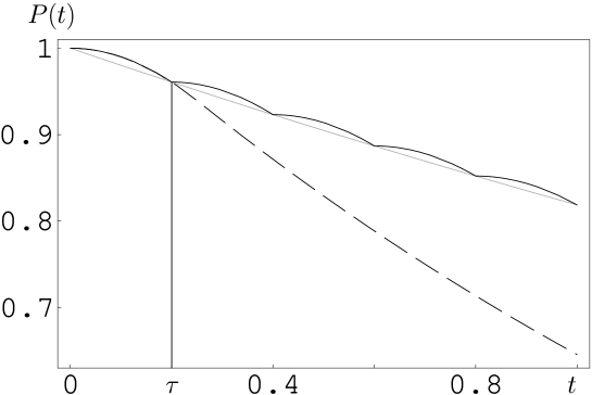
Figure 1: Quantum Zeno effect due to “pulsed” measurements. The dashed (full) line is the survival probability without (with) measurements. ($t$ in arbitrary units.)

Let $H$ be the total Hamiltonian of a quantum system. The survival amplitude and probability of the system in state $|\psi_{0}\rangle$ are

$${\cal A}(t) = \langle\psi_{0}|\psi_{t}\rangle=\langle\psi_{0}|e^{-iHt}|\psi_{0}\rangle, 2.1$$ ()

$$P(t) = |{\cal A}(t)|^{2}=|\langle\psi_{0}|e^{-iHt}|\psi_{0}\rangle|^{2}, 2.2$$ ()

respectively. An elementary expansion yields a quadratic behavior at short times

$$P(t)\sim 1-t^{2}/\tau_{\rm Z}^{2}\sim e^{-t^{2}/\tau_{\rm Z}^{2}},\qquad\tau_{\rm Z}^{-2}\equiv\langle\psi_{0}|H^{2}|\psi_{0}\rangle-\langle\psi_{0}|H|\psi_{0}\rangle^{2}. 2.3$$ ()

It is often claimed that $\tau_{\rm Z}$ (“Zeno time”) yields a quantitative estimate of the short-time behavior. This is misleading in many situations: $\tau_{\rm Z}$ is only the convexity of $P(t)$ in the origin. This is a central observation and will be corroborated by several examples. See [20] for an exhaustive discussion.

Figure 2: Short-time evolution of phase and probability.

Observe that if one divides the Hamiltonian into a free and an interaction part

$$H=H_{0}+H_{\rm I} 2.4$$ ()

and sets (for additional details and mathematical rigor, see [14, 20, 21])

$$H_{0}|{\psi_{0}}\rangle=E_{0}|{\psi_{0}}\rangle,\quad\langle{\psi_{0}}|H_{\rm I}|{\psi_{0}}\rangle=0, 2.5$$ ()

the Zeno time reads

$$\tau_{\rm Z}^{-2}=\langle\psi_{0}|H_{\rm I}^{2}|\psi_{0}\rangle 2.6$$ ()

and depends only on the off-diagonal part of the Hamiltonian.

In order to get QZE, we perform $N$ measurements at time intervals $\tau$, to check whether the system is still in its initial state. The survival probability after the measurements reads

$$P^{(N)}(t) = P(\tau)^{N}=P(t/N)^{N} 2.7$$ ()

$$\stackrel{{\scriptstyle N\;{\rm large}}}{{\longrightarrow}}\left[1-(t/N\tau_{\rm Z})^{2}\right]^{N}\sim\exp(-t^{2}/N\tau_{\rm Z}^{2})\stackrel{{\scriptstyle N\rightarrow\infty}}{{\longrightarrow}}1,$$

where $t=N\tau$ is the total duration of the experiment. The Zeno evolution is pictorially represented in Figure 1.

The QZE is a direct consequence of the Schrödinger equation that yields quadratic behavior of the survival probability at short times: in a short time $\delta\tau\sim 1/N$, the phase of the wave function evolves like $\mbox{O}(\delta\tau)$, while the probability changes by $\mbox{O}(\delta\tau^{2})$, so that

$$P^{(N)}(t)\sim\left[1-\mbox{O}(1/N^{2})\right]^{N}\stackrel{{\scriptstyle N\rightarrow\infty}}{{\longrightarrow}}1. 2.8$$ ()

This is sketched in Figure 2 and is a very general feature of the Schrödinger equation. As a matter of fact, many other fundamental physical equations share the same property.

3 A theorem: from quantum Zeno to inverse quantum Zeno

We rewrite ($2.7$) as

$$P^{(N)}(t)=P(\tau)^{N}=\exp(N\log P(\tau))=\exp(-\gamma_{\rm eff}(\tau)t), 3.1$$ ()

where we introduced an effective decay rate [22, 20]

$$\gamma_{\rm eff}(\tau)\equiv-\frac{1}{\tau}\log P(\tau)=-\frac{2}{\tau}\log|{\cal A}(\tau)|=-\frac{2}{\tau}\mbox{Re}[\log{\cal A}(\tau)]. 3.2$$ ()

For instance, for times $\tau$ such that the quadratic behavior ($2.3$) is valid with good approximation, one easily checks that

$$\gamma_{\rm eff}(\tau)\sim\tau/\tau_{\rm Z}^{2},\qquad(\tau\to 0) 3.3$$ ()

is a linear function of $\tau$. We now concentrate our attention on a truly unstable system, with “natural” decay rate $\gamma$, given by the Fermi “golden” rule [12]. We ask whether it is possible to find a finite time $\tau^{*}$ such that

$$\gamma_{\rm eff}(\tau^{*})=\gamma. 3.4$$ ()

If such a time exists, then by performing measurements at time intervals $\tau^{*}$ the system decays according to its “natural” lifetime, as if no measurements were performed. The related concept of “jump” time was considered in [23]. See also [14, 24].

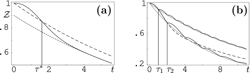
Figure 3: ${\cal Z}<1$. (a) Determination of $\tau^{*}$. (b) Quantum Zeno vs inverse quantum Zeno (“Heraclitus”) effect.

By Eqs. ($3.4$) and ($3.2$) one gets

$$P(\tau^{*})=e^{-\gamma\tau^{*}}, 3.5$$ ()

i.e., $\tau^{*}$ is the intersection between the curves $P(t)$ and $e^{-\gamma t}$. In the situation depicted in Figure 3(a) such a time $\tau^{*}$ exists: the full line is the survival probability and the dashed line the exponential $e^{-\gamma t}$ [the dotted line is the asymptotic exponential ${\cal Z}e^{-\gamma t}$, see ($3.6$) in the following]. The physical meaning of $\tau^{*}$ can be understood by looking at Figure 3(b), where the dashed line represents a typical behavior of the survival probability $P(t)$ when no measurement is performed: the short-time Zeno region is followed by an approximately exponential decay with a natural decay rate $\gamma$. When measurements are performed at time intervals $\tau$, we get the effective decay rate $\gamma_{\rm eff}(\tau)$. The full lines represent the survival probabilities and the dotted lines their exponential interpolations, according to ($3.1$). If $\tau=\tau_{1}<\tau^{*}$ one obtains QZE. Vice versa, if $\tau=\tau_{2}>\tau^{*}$, one obtains IZE. If $\tau=\tau^{*}$ one recovers the natural lifetime, according to ($3.4$): in this sense, $\tau^{*}$ can be viewed as a transition time from a quantum Zeno to an inverse quantum Zeno regime. Paraphrasing Misra and Sudarshan [2] we can say that $\tau^{*}$ determines the transition from Zeno (who argued that a sped arrow, if observed, does not move) to Heraclitus (who replied that everything flows).

Figure 4: ${\cal Z}>1$. The full line is the survival probability, the dashed line the renormalized exponential $e^{-\gamma t}$ and the dotted line the asymptotic exponential ${\cal Z}e^{-\gamma t}$. (a) If $P(t)$ and $e^{-\gamma t}$ do not intersect, a finite solution $\tau^{*}$ does not exist. (b) If $P(t)$ and $e^{-\gamma t}$ intersect, a finite solution $\tau^{*}$ exists. (In this case there are always at least two intersections.)

We stress that it is not always possible to determine $\tau^{*}$: Eq. ($3.4$) may have no finite solutions. Indeed, for sufficiently long times the survival probability of an unstable system reads with very good approximation

$$P(t)=|{\cal A}(t)|^{2}\simeq{\cal Z}e^{-\gamma t}, 3.6$$ ()

where ${\cal Z}$, the intersection of the asymptotic exponential with the $t=0$ axis, is the wave function renormalization and is given by the square modulus of the residue of the pole of the propagator [14, 20, 22].

A sufficient condition for the existence of a solution $\tau^{*}$ of Eq. ($3.4$) is that ${\cal Z}<1$. This is easily proved by graphical inspection. The case ${\cal Z}<1$ is shown in Figure 3(a): $P(t)$ and $e^{-\gamma t}$ must intersect, since according to ($3.6$), $P(t)\sim{\cal Z}e^{-\gamma t}$ for large $t$, and a finite solution $\tau^{*}$ can always be found. The other case, ${\cal Z}>1$, is shown in Figure 4: a solution may or may not exist, depending on the features of the model investigated. There are also situations (e.g., oscillatory systems, whose Poincaré time is finite) where $\gamma$ and ${\cal Z}$ cannot be defined [20]. The (existence of a) transition from Zeno to inverse Zeno is therefore a complex, model-dependent problem, that requires careful investigation. The theorem shown in this section gives a simple criterion for the occurrence of such a transition.

4 Continuous measurement

We now introduce some alternative descriptions of a measurement process and discuss the notion of continuous measurement. This is to be contrasted with the idea of pulsed measurements, discussed in Section 2 and hinging upon von Neumann’s projections [19].

Let us mimic the action of an external apparatus by the non Hermitian Hamiltonian

$$H_{\rm I}=\pmatrix{0&\Omega\cr\Omega&-i2V}=-iV{\bf 1}+\mbox{\boldmath$h$}\cdot\mbox{\boldmath$\sigma$},\qquad\mbox{\boldmath$h$}=(\Omega,0,iV)^{T}, 4.1$$ ()

that yields Rabi oscillations of frequency $\Omega$, but at the same time absorbs away the $|-\rangle=\left({0\atop 1}\right)$ component of the quantum state, performing in this way a “measurement.” Due to the non Hermitian features of this description, probabilities are not conserved: we are concentrating our attention only on the $|+\rangle=\left({1\atop 0}\right)$ component.

An elementary calculation yields the evolution operator

$$e^{-iH_{\rm I}t}=e^{-Vt}\left[\cosh(ht)-i\frac{\mbox{\boldmath$h$}\cdot\mbox{\boldmath$\sigma$}}{h}\sinh(ht)\right], 4.2$$ ()

where $h=\sqrt{V^{2}-\Omega^{2}}$ and we supposed $V>\Omega$. Let the system be initially prepared in state $|\psi_{0}\rangle=|+\rangle$: the survival amplitude reads

$${\cal A}(t) = \langle\psi_{0}|e^{-iH_{\rm I}t}|\psi_{0}\rangle 4.3$$ ()

$$= e^{-Vt}\left[\cosh(\sqrt{V^{2}-\Omega^{2}}t)+\frac{V}{\sqrt{V^{2}-\Omega^{2}}}\sinh(\sqrt{V^{2}-\Omega^{2}}t)\right].$$

The above results are exact and display some general aspects of the quantum Zeno dynamics. The survival probability $P(t)=|{\cal A}(t)|^{2}$ is shown in Figure 5 for $V=0.4,2,10\Omega$.

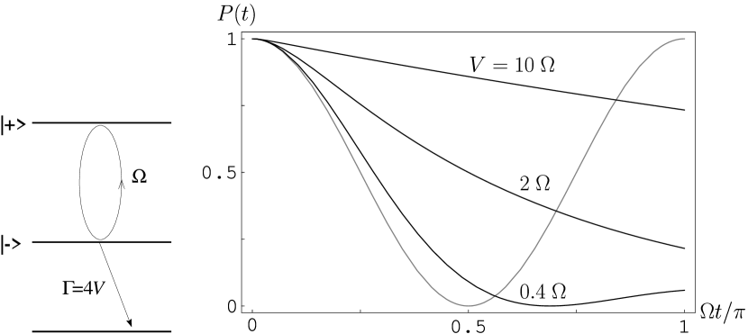
Figure 5: Survival probability for a system undergoing Rabi oscillations in presence of absorption ($V=0.4,2,10\Omega$). The gray line is the undisturbed evolution ($V=0$).

As expected, probability is (exponentially) absorbed away as $t\to\infty$. However, for large $V(\gg\Omega)$ the survival probability becomes

$$P(t)\sim\left(1+\frac{\Omega^{2}}{2V}\right)\exp\left(-\frac{\Omega^{2}}{V}t\right), 4.4$$ ()

and the effective decay rate $\gamma_{\rm eff}(V)=\Omega^{2}/V$ becomes smaller, eventually halting the “decay” of the initial state and yielding an interesting example of QZE: a larger $V$ entails a more “effective” measurement of the initial state. Notice that the expansion ($4.4$) becomes valid very quickly, on a time scale of order $V^{-1}$.

The non Hermitian Hamiltonian ($4.1$) “summarizes” the evolution engendered by a Hermitian Hamiltonian acting on a larger Hilbert space, if attention is restricted to the subspace spanned by $\{|{+}\rangle,|{-}\rangle\}$: indeed, let

$$H=\Omega(|{+}\rangle\langle{-}|+|{-}\rangle\langle{+}|)+\int d\omega\;\omega|{\omega}\rangle\langle{\omega}|+\sqrt{\frac{\Gamma}{2\pi}}\int d\omega\;(|{-}\rangle\langle{\omega}|+|{\omega}\rangle\langle{-}|), 4.5$$ ()

describing a two level system coupled to the photon field in the rotating-wave approximation. By writing the state of the system at time $t$ as

$$|{\psi_{t}}\rangle={\cal A}(t)|{+}\rangle+y(t)|{-}\rangle+\int d\omega\;z(\omega,t)|{\omega}\rangle, 4.6$$ ()

a straightforward manipulation yields

$$i\dot{\cal A}(t) = \Omega y(t),$$

$$i\dot{y}(t) = -i\frac{\Gamma}{2}y+\Omega{\cal A}(t). 4.7$$ ()

These are the same equations of motion obtained from the non Hermitian Hamiltonian

$$H=\Omega(|{+}\rangle\langle{-}|+|{-}\rangle\langle{+}|)-i\frac{\Gamma}{2}|{-}\rangle\langle{-}|. 4.8$$ ()

which is the same as ($4.1$) when one sets $\Gamma=4V$. QZE is obtained by increasing $\Gamma$ in ($4.5$)-($4.8$): a larger coupling to the environment (photons) leads to a more effective “continuous” observation on the system (quicker response of the environment), and as a consequence to a slower decay.

As one can see, the only effect of the continuum in ($4.5$) is the appearance of the imaginary frequency $-i\Gamma/2$. This is ascribable to the “flatness” of the continuum [there is no form factor or frequency cutoff in the last term of Eq. ($4.5$)], which yields a purely exponential (Markovian) decay of $y(t)$.

The process described in this section can be viewed as a “continuous” measurement performed on the initial state $|{+}\rangle$: state $|{-}\rangle$ is indeed continuously monitored with a response time $1/\Gamma$ and as soon as it becomes populated, it is detected within a time $1/\Gamma$. The “effectiveness” $\Gamma=4V$ of the observation can be compared to the frequency $\tau^{-1}=(t/N)^{-1}$ of measurements in the “pulsed” formulation. Indeed, for large values of $\Gamma$ one gets from Eq. ($4.4$)

$$\gamma_{\rm eff}(\Gamma)\sim\frac{4\Omega^{2}}{\Gamma}=\frac{4}{\tau_{\rm Z}^{2}\Gamma},\qquad(\Gamma\to\infty), 4.9$$ ()

which, compared with Eq. ($3.3$), yields an interesting relation between continuous and pulsed measurements

$$\Gamma\simeq 4/\tau=4N/t. 4.10$$ ()

In a Zeno context, the strength of the coupling can therefore be viewed as an inverse characteristic time. The effective lifetime $\gamma_{\rm eff}$ is then a function of the time interval $\tau$ between successive (pulsed) measurements or, alternatively, of the strength $\Gamma$ of the (continuous) measurement. This also leads to a novel definition of QZE (and IZE) [20]. The relation between “pulsed” and “continuous” measurements in the context of QZE was first emphasized by Schulman [17].

5 Continuous “Rabi” measurement

Let us now analyze a different situation, by coupling state $|-\rangle$ to another state $|M\rangle$, that will play the role of measuring apparatus. This will clarify that absorption and/or probability leakage to the environment (like those investigated in the previous section) are not fundamental requisites to obtain QZE.

The (Hermitian) Hamiltonian is

$$H_{\rm I}=\Omega(|+\rangle\langle-|+|-\rangle\langle+|)+K(|-\rangle\langle M|+|M\rangle\langle-|)=\pmatrix{0&\Omega&0\cr\Omega&0&K\cr 0&K&0}, 5.1$$ ()

where $K\in\mathbb{R}$ is the strength of the coupling to the new level $M$ and

$$\langle+|=(1,0,0),\quad\langle-|=(0,1,0),\quad\langle M|=(0,0,1). 5.2$$ ()

This is probably the simplest way to include an “external” apparatus in our description: as soon as the system is in $|-\rangle$ it undergoes Rabi oscillations to $|M\rangle$. Similar examples were considered by other authors [18]. We expect level $|M\rangle$ to perform better as a measuring apparatus when the strength $K$ of the coupling increases.

The initial state is $|\psi_{0}\rangle=|+\rangle$ and after a straightforward calculation one obtains the survival probability in state $|+\rangle$

$$P(t)=\frac{1}{(K^{2}+\Omega^{2})^{2}}\left[K^{2}+\Omega^{2}\cos(\sqrt{K^{2}+\Omega^{2}}t)\right]^{2}. 5.3$$ ()

This is shown in Figure 6 for $K=1,3,9\Omega$.

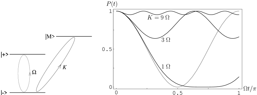
Figure 6: Survival probability for a continuous Rabi “measurement” with $K=1,3,9\Omega$: quantum Zeno effect.

We notice that for large $K$ the state of the system does not differ much from the initial state: as $K$ is increased, level $|M\rangle$ performs a better “observation” of the state of the system, hindering transitions from $|+\rangle$ to $|-\rangle$. This can be viewed as a QZE due to a “continuous,” yet Hermitian observation performed by level $|M\rangle$.

This simple example enables one to make an important observation. The Zeno time is easily computed and turns out to be much longer than the Poincaré time $T_{\rm P}$ (we are assuming $K\gg\Omega$)

$$\tau_{\rm Z}=\Omega^{-1}\gg T_{\rm P}=\mbox{O}(K^{-1}). 5.4$$ ()

As a matter of fact, $\tau_{\rm Z}$ yields only the convexity of the survival probability in the origin: in general, the short-time quadratic evolution of the system is much shorter. This contradicts many erroneous claims in the literature of the last few years.

One can also obtain a relation similar to ($4.10$):

$$K\simeq\frac{\sqrt{2N}}{t}: 5.5$$ ()

again, strong coupling is equivalent to frequent measurements [20].

A final comment is in order. All the situations analyzed in Sections 4 and 5 lead to QZE but never to IZE. The reason for this is profound and lies in the absence of the form factors of the interactions. The importance of form factors and the role they play in this context is discussed in [20, 22] and will be clarified in the following section.

6 Influence of form factors

Consider the Hamiltonian

$$H_{\rm decay}=H_{0}+H_{\rm I}=\omega_{\rm in}|{\rm in}\rangle\langle{{\rm in}}|+\sum_{n}\omega_{n}|{n}\rangle\langle{n}|+\sum_{n}\left(\phi_{n}|{n}\rangle\langle{{\rm in}}|+\phi^{*}_{n}|{{\rm in}}\rangle\langle{n}|\right), 6.1$$ ()

with $\langle{n}|n^{\prime}\rangle=\delta_{nn^{\prime}}$, $\langle{\rm in}|\rm in\rangle=1$ and $\langle{n}|{\rm in}\rangle=0$, describing an initial state $|{\rm in}\rangle$ coupled to many discrete states (we will eventually consider the continuum limit in order to get a decay process). The coupling is not “flat:” there is a form factor $\phi_{n}$. The state of the system at time $t$ is

$$|{\psi_{t}}\rangle={\cal A}(t)e^{-i\omega_{\rm in}t}|{\rm in}\rangle+\sum_{n}z_{n}(t)|{n}\rangle 6.2$$ ()

and the Schrödinger equation, with the initial condition $|{\psi_{0}}\rangle=|{\rm in}\rangle$, yields

$$\dot{\cal A}(t)=-\sum_{n}|\phi_{n}|^{2}\int_{0}^{t}ds\;\exp[-i(\omega_{n}-\omega_{\rm in})s]{\cal A}(t-s). 6.3$$ ()

Observe that ${\cal A}(t)$ contains non-exponential contributions [25].

Let the (pulsed) measurements be performed at time intervals much shorter than the natural lifetime, $\tau\ll 1/\gamma$. Since $\tau$ is very small, ${\cal A}(\tau)\simeq{\cal A}(0)=1$, and

$$\log{\cal A}(\tau)\sim{\cal A}(\tau)-1={\cal A}(\tau)-{\cal A}(0)=\int_{0}^{\tau}dt\;\dot{\cal A}(t), 6.4$$ ()

so that the expression $\gamma_{\rm eff}(\tau)=-(2/\tau)\mbox{Re}\{\log{\cal A}(\tau)\}$ in ($3.2$) yields

$$\gamma_{\rm eff}(\tau) \sim \frac{2}{\tau}\;\mbox{Re}\sum_{n}|\phi_{n}|^{2}\int_{0}^{\tau}dt\int_{0}^{t}ds\;e^{-i(\omega_{n}-\omega_{\rm in})s}{\cal A}(t-s) 6.5$$ ()

$$\sim \frac{2}{\tau}\sum_{n}|\phi_{n}|^{2}\mbox{Re}\int_{0}^{\tau}dt\int_{0}^{t}ds\;\exp[-i(\omega_{n}-\omega_{\rm in})s],$$

where we used again ${\cal A}(\tau)\simeq 1$. By performing the integration

$$\gamma_{\rm eff}(\tau)=\tau\sum_{n}|\phi_{n}|^{2}\frac{\sin^{2}\left(\frac{(\omega_{n}-\omega_{\rm in})\tau}{2}\right)}{\left(\frac{(\omega_{n}-\omega_{\rm in})\tau}{2}\right)^{2}} 6.6$$ ()

and introducing the spectral density function (form factor)

$$\kappa(\omega)=\sum_{n}\delta(\omega-\omega_{n})|\phi_{n}|^{2}, 6.7$$ ()

whose support is the spectrum $\{\omega_{n}\}_{n}$, we get

$$\gamma_{\rm eff}(\tau)=\tau\int_{\omega_{0}}^{\infty}d\omega\;\kappa(\omega)\frac{\sin^{2}\left(\frac{(\omega-\omega_{\rm in})\tau}{2}\right)}{\left(\frac{(\omega-\omega_{\rm in})\tau}{2}\right)^{2}}, 6.8$$ ()

where $\omega_{0}$ is the ground state energy. This result was first obtained by Kofman and Kurizki, last article in [7]. We assume $\omega_{0}<\omega_{\rm in}$, in order to have a decaying initial state $|{\rm in}\rangle$. Note that in the continuum limit the energies $\omega_{n}$ form a continuum and the form factor $\kappa(\omega)$ becomes an ordinary function of $\omega$

$$\kappa(\omega)=\rho(\omega)|\varphi(\omega)|^{2}, 6.9$$ ()

where $\rho$ is the state density function and $\varphi$ the rescaled matrix element. A typical behavior of the form factor is shown in Figure 7: observe that $\kappa(\omega<\omega_{0})=0$ and $\kappa(\omega>\omega_{0}+\Lambda)\simeq 0$, where $\Lambda$ is a natural cutoff.

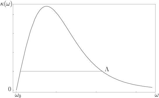
Figure 7: Typical behavior of the form factor $\kappa(\omega)$.

A pictorial representation of the integral ($6.8$) is given in Figure 8(a): the detector “response” function ${\rm sinc}^{2}[(\omega-\omega_{\rm in})\tau/2]$ [where ${\rm sinc}(x)\equiv\sin x/x$] is modulated by the form factor $\kappa(\omega)$.

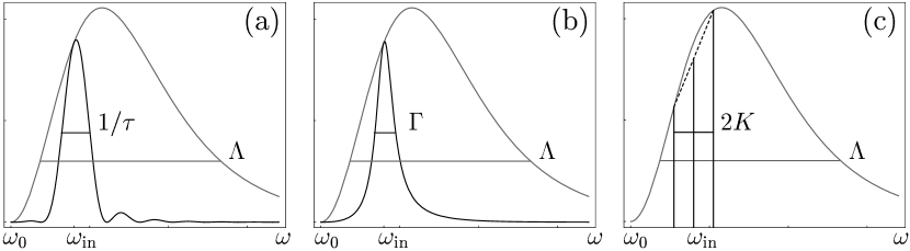
Figure 8: Form factor $\kappa(\omega)$ and detector “response” function for: (a) pulsed measurements, Eq. ($6.8$), with detector response function ${\rm sinc}^{2}[(\omega-\omega_{\rm in})\tau/2]$; (b) continuous measurement, Eq. ($6.17$), with detector response function $(\Gamma/2)^{2}/[(\omega-\omega_{\rm in})^{2}+(\Gamma/2)^{2}]$; (c) “Rabi” measurement, Eq. ($6.23$), with detector response function $[\delta(\omega-\omega_{\rm in}-K)+\delta(\omega-\omega_{\rm in}+K)]$. The gray line is a typical form factor and the full line represents the function in the integral, given by the appropriate response function times the form factor.

By using the asymptotic properties of sinc${}^{2}(x)$, we get

$$\gamma_{\rm eff}(\tau) \simeq 2\pi\kappa(\omega_{\rm in})=\gamma\qquad\mbox{for}\;\;\tau\gg 1/\Lambda, 6.10$$ ()

$$\gamma_{\rm eff}(\tau) \simeq \tau\int_{\omega_{0}}^{\infty}d\omega\;\kappa(\omega)=\frac{\tau}{\tau_{\rm Z}^{2}}\qquad\mbox{for}\;\;\tau\ll 1/\Lambda, 6.11$$ ()

where Eqs. ($6.7$), ($6.1$) and ($2.6$) were used to obtain

$$\int_{\omega_{0}}^{\infty}d\omega\;\kappa(\omega)=\sum_{n}|\phi_{n}|^{2}=\langle{\rm in}|H_{\rm I}^{2}|{\rm in}\rangle=\tau_{\rm Z}^{-2}. 6.12$$ ()

The first result ($6.10$) was to be expected: if the time interval $\tau$ between successive pulsed measurements is long enough, one recovers the “natural” lifetime, computed according to the Fermi “golden” rule. The second result ($6.11$) is interesting and generalizes ($3.3$), providing a timescale $\Lambda^{-1}$ for its range of validity. Notice that $\gamma_{\rm eff}$ is a linear function of $\tau$ in this range. A typical behavior of $\gamma_{\rm eff}(\tau)$, for a form factor like that in Figure 7, is shown in Figure 9: for $\tau<\tau^{*}$, one has $\gamma_{\rm eff}<\gamma$ and therefore QZE. Viceversa, for $\tau>\tau^{*}$, one has $\gamma_{\rm eff}>\gamma$ and therefore IZE [22, 20].

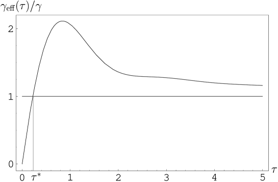
Figure 9: Effective decay rate $\gamma_{\rm eff}(\tau)$: typical behavior for systems exhibiting a QZE-IZE transition. The horizontal line shows the natural decay rate $\gamma$: its intersection with $\gamma_{\rm eff}(\tau)$ yields the transition time $\tau^{*}$, solution of Eq. ($3.4$). Notice the presence of a linear region for small values of $\tau$, according to Eq. ($6.11$). A Zeno (inverse Zeno) effect is obtained for $\tau<\tau^{*}$ ($\tau>\tau^{*}$). For large $\tau$, the asymptotic value of the curve is $\gamma$, as expected from Eq. ($6.10$).

The previous analysis and results are valid for pulsed measurements. Let us consider now a continuous measurement process. This is accomplished, for instance, by adding to ($6.1$) the following Hamiltonian

$$H_{\rm meas}(\Gamma)=\sqrt{\frac{\Gamma}{2\pi}}\sum_{n}\int d\omega^{\prime}\;(|{n}\rangle\langle{n,\omega^{\prime}}|+|{n,\omega^{\prime}}\rangle\langle{n}|)+\int d\omega^{\prime}\;|{\omega^{\prime}}\rangle\langle{\omega^{\prime}}|: 6.13$$ ()

as soon as state $|{n}\rangle$ is populated, it is coupled to a boson of frequency $\omega^{\prime}$ (notice that the coupling has no form factor). By following a reasoning identical to that of Section 4, one can show that the dynamics of the Hamitonian ($6.1$) $+$ ($6.13$), in the relevant subspace, is generated by

$$H=\omega_{\rm in}|{\rm in}\rangle\langle{{\rm in}}|+\sum_{n}\left(\omega_{n}-i\frac{\Gamma}{2}\right)|{n}\rangle\langle{n}|+\sum_{n}\left(\phi_{n}|{n}\rangle\langle{{\rm in}}|+\phi^{*}_{n}|{{\rm in}}\rangle\langle{n}|\right) 6.14$$ ()

and a better continuous observation on the system is obtained by increasing $\Gamma$, like in Section 4. With the substitution $\omega_{n}\to\omega_{n}-i\Gamma/2$, Eq. ($6.3$) reads

$$\dot{\cal A}(t)=-\sum_{n}|\phi_{n}|^{2}\int_{0}^{t}ds\;\exp[-i(\omega_{n}-\omega_{\rm in}-i\Gamma/2)s]{\cal A}(t-s). 6.15$$ ()

For $t\gg 1/\Lambda$ (and not extremely large), where $\Lambda$ is the cutoff of the form factor (see Figure 7), the decay is exponential with very high accuracy and the decay rate is given by

$$\gamma_{\rm eff}(\Gamma)=2\sum_{n}|\phi_{n}|^{2}\mbox{Re}\int_{0}^{\infty}dt\;e^{-i(\omega_{n}-\omega_{\rm in}-i\Gamma/2)t}=\frac{4}{\Gamma}\sum_{n}|\phi_{n}|^{2}\frac{\frac{\Gamma^{2}}{4}}{(\omega_{n}-\omega_{\rm in})^{2}+\frac{\Gamma^{2}}{4}}. 6.16$$ ()

In the continuum limit, ($6.16$) is expressed in terms of the spectral density ($6.9$):

$$\gamma_{\rm eff}(\Gamma)=\frac{4}{\Gamma}\int_{\omega_{0}}^{\infty}d\omega\;\kappa(\omega)\frac{\frac{\Gamma^{2}}{4}}{(\omega-\omega_{\rm in})^{2}+\frac{\Gamma^{2}}{4}}, 6.17$$ ()

which is the analog of formula ($6.8$) for continuous measurement. The function in the above integral is represented in Figure 8(b). The asymptotic values are

$$\gamma_{\rm eff}(\Gamma) \simeq \gamma\quad\mbox{for}\quad\Gamma\ll\Lambda, 6.18$$ ()

$$\gamma_{\rm eff}(\Gamma) \simeq \frac{4}{\tau_{\rm Z}^{2}\Gamma}\quad\mbox{for}\quad\Gamma\gg\Lambda 6.19$$ ()

and must be compared to ($6.10$)-($6.11$). Once again, the result ($6.18$) was to be expected: if the coupling $\Gamma$ to the external field is weak enough (as compared to $\Lambda$) the system decays according to its “natural” lifetime, computed according to the Fermi “golden” rule. On the other hand, Eq. ($6.19$) is interesting and yields again ($4.10$) [via ($6.11$)] in a more general context. Furthermore, when $\Gamma$ varies between $0$ and $\infty$, $\gamma_{\rm eff}(\Gamma)$ describes a curve very similar to that relative to pulsed measurements and represented in Figure 9.

Finally, one can also consider the continuous “Rabi” measurement of Sec. 5, by adding to ($6.1$) the following Hamiltonian

$$H_{\rm meas}(K)=K\sum_{n}(|{n}\rangle\langle{n,M}|+|{n,M}\rangle\langle{n}|)+\sum_{n}\omega_{n}|{n,M}\rangle\langle{n,M}|, 6.20$$ ()

with $\langle{n,M}|n^{\prime},M\rangle=\delta_{nn^{\prime}}$, $\langle{n}|n^{\prime},M\rangle=0$ and $\langle{\rm in}|n,M\rangle=0$: as soon as state $|{n}\rangle$ is populated, it undergoes Rabi oscillations to the orthogonal state $|{n,M}\rangle$. The Schrödinger equation yields

$$\dot{\cal A}(t)=-\sum_{n}|\phi_{n}|^{2}\int_{0}^{t}ds\;\exp[-i(\omega_{n}-\omega_{\rm in})s]\cos(Ks)\;{\cal A}(t-s), 6.21$$ ()

which is to be compared with Eqs. ($6.3$) and ($6.15$). The exponential decay rate reads now

$$\gamma_{\rm eff}(K) = 2\sum_{n}|\phi_{n}|^{2}\mbox{Re}\int_{0}^{\infty}dt\;e^{-i(\omega_{n}-\omega_{\rm in})t}\cos(Kt) 6.22$$ ()

$$= \pi\sum_{n}|\phi_{n}|^{2}\left[\delta(\omega_{n}-\omega_{\rm in}-K)+\delta(\omega_{n}-\omega_{\rm in}+K)\right]$$

and is expressed in terms of the spectral density function

$$\gamma_{\rm eff}(K) = \pi\int_{\omega_{0}}^{\infty}d\omega\;\kappa(\omega)\left[\delta(\omega-\omega_{\rm in}-K)+\delta(\omega-\omega_{\rm in}+K)\right] 6.23$$ ()

$$= \pi\left[\kappa(\omega_{\rm in}+K)+\kappa(\omega_{\rm in}-K)\right].$$

The decay rate is the arithmetic mean between two “free” decay rates, from initial states with shifted initial energies $\omega_{\rm in}\pm K$, into the same continuum [10]. This is shown in Figure 8(c). The asymptotic values read

$$\gamma_{\rm eff}(K) \simeq \gamma\quad\mbox{for}\quad K\ll\Lambda, 6.24$$ ()

$$\gamma_{\rm eff}(K) = \pi\kappa(\omega_{\rm in}+K)\quad\mbox{for}\quad K\gg\Lambda, 6.25$$ ()

The physical meaning of the first expression is apparent. Note that the second equation is already exact for $K>\omega_{\rm in}-\omega_{0}$, because $\kappa(\omega)$ vanishes identically for $\omega<\omega_{0}$. Note also that for $K\to\infty$ (infinitely strong Rabi measurement) $\gamma_{\rm eff}(K)$ tends to zero exactly like the form factor (QZE).

In the next section we will consider a physical situation in which a decaying system is actually “observed” via a Rabi oscillation and will see that for sensible values of the parameters the decay is enhanced (IZE).

7 Three-level system in a laser field

We now analyze a realistic situation in which a continuous observation performed by a laser field leads to an inverse quantum Zeno effect. We look at the temporal behavior of a three-level system (such as an atom or a molecule), where level $|1\rangle$ is the ground state and levels $|2\rangle$, $|3\rangle$ are two excited states [16]. See Figure 10. The system is initially prepared in level $|2\rangle$ and if it follows its natural evolution, it will decay to level $|1\rangle$. The decay will be (approximately) exponential and characterized by a certain lifetime, that can be calculated from the Fermi “golden” rule. But if one shines on the system an intense laser field, tuned at the transition frequency 3-1, the decay is enhanced (inverse quantum Zeno effect) [10].

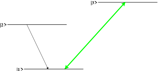
Figure 10: Level configuration

We consider the Hamiltonian ($\hbar=c=1$)

$$H = H_{0}+H_{\rm int} 7.1$$ ()

$$= \omega_{0}|2\rangle\langle 2|+\Omega_{0}|3\rangle\langle 3|+\sum_{\mbox{\boldmath\scriptsize$k$},\lambda}\omega_{k}a^{\dagger}_{\mbox{\boldmath\scriptsize$k$}\lambda}a_{\mbox{\boldmath\scriptsize$k$}\lambda}+\sum_{\mbox{\boldmath\scriptsize$k$},\lambda}\left(\phi_{\mbox{\boldmath\scriptsize$k$}\lambda}a_{\mbox{\boldmath\scriptsize$k$}\lambda}^{\dagger}|1\rangle\langle 2|+\phi_{\mbox{\boldmath\scriptsize$k$}\lambda}^{*}a_{\mbox{\boldmath\scriptsize$k$}\lambda}|2\rangle\langle 1|\right)$$

$$+\sum_{\mbox{\boldmath\scriptsize$k$},\lambda}\left(\Phi_{\mbox{\boldmath\scriptsize$k$}\lambda}a_{\mbox{\boldmath\scriptsize$k$}\lambda}^{\dagger}|1\rangle\langle 3|+\Phi_{\mbox{\boldmath\scriptsize$k$}\lambda}^{*}a_{\mbox{\boldmath\scriptsize$k$}\lambda}|3\rangle\langle 1|\right),$$

where the first two terms are the free Hamiltonian of the 3-level atom (whose states $|i\rangle$ $(i=1,2,3)$ have energies $E_{1}=0$, $\omega_{0}=E_{2}-E_{1}>0$, $\Omega_{0}=E_{3}-E_{1}>0$), the third term is the free Hamiltonian of the EM field ($\lambda$ being a discrete index that labels the photon polarization) and the last two terms describe the $1\leftrightarrow 2$ and $1\leftrightarrow 3$ transitions in the rotating wave approximation, respectively. (See Figure 10.) States $|2\rangle$ and $|3\rangle$ are chosen so that no transition between them is possible (e.g., because of selection rules). The matrix elements of the interaction Hamiltonian read

$$\phi_{\mbox{\boldmath\scriptsize$k$}\lambda} = \frac{e}{\sqrt{2\epsilon_{0}V\omega}}\int d^{3}x\;e^{-i\mbox{\boldmath\scriptsize$k$}\cdot\mbox{\boldmath\scriptsize$x$}}\mbox{\boldmath$\epsilon$}_{\mbox{\boldmath\scriptsize$k$}\lambda}^{*}\cdot\mbox{\boldmath$j$}_{12}(\mbox{\boldmath$x$}),$$

$$\Phi_{\mbox{\boldmath\scriptsize$k$}\lambda} = \frac{e}{\sqrt{2\epsilon_{0}V\omega}}\int d^{3}x\;e^{-i\mbox{\boldmath\scriptsize$k$}\cdot\mbox{\boldmath\scriptsize$x$}}\mbox{\boldmath$\epsilon$}_{\mbox{\boldmath\scriptsize$k$}\lambda}^{*}\cdot\mbox{\boldmath$j$}_{13}(\mbox{\boldmath$x$}), 7.2$$ ()

where $-e$ is the electron charge, $\epsilon_{0}$ the vacuum permittivity, $V$ the volume of the box, $\omega=|\mbox{\boldmath$k$}|$, $\mbox{\boldmath$\epsilon$}_{\mbox{\boldmath\scriptsize$k$}\lambda}$ the photon polarization and $\mbox{\boldmath$j$}_{\rm fi}$ the transition current of the radiating system. For example, in the case of an electron in an external field, we have $\mbox{\boldmath$j$}_{\rm fi}=\psi_{\rm f}^{\dagger}\mbox{\boldmath$\alpha$}\psi_{\rm i}$ where $\psi_{\rm i}$ and $\psi_{\rm f}$ are the wavefunctions of the initial and final state, respectively, and $\alpha$ is the vector of Dirac matrices. For the sake of generality we are using relativistic matrix elements, but our analysis can also be performed with nonrelativistic ones $\mbox{\boldmath$j$}_{\rm fi}=\psi_{\rm f}^{*}\mbox{\boldmath$p$}\psi_{\rm i}/m_{e}$, where $\mbox{\boldmath$p$}/m_{e}$ is the electron velocity.

We only give here the main results. The detailed calculation can be found in [10]. The temporal evolution is found by solving the time-dependent Schrödinger equation

$$i\frac{d}{dt}|\psi(t)\rangle=H(t)|\psi(t)\rangle, 7.3$$ ()

for the states [$|i;n_{\mbox{\boldmath\scriptsize$k$}\lambda}\rangle$ = atom in state $|i\rangle$ and $n_{\mbox{\boldmath\scriptsize$k$}\lambda}$ $(\mbox{\boldmath$k$},\lambda)$-photons]

$$|\psi(t)\rangle={\cal A}(t)|2;0\rangle+{\sum_{\mbox{\boldmath\scriptsize$k$},\lambda}}^{\prime}y_{\mbox{\boldmath\scriptsize$k$}\lambda}(t)|1;1_{\mbox{\boldmath\scriptsize$k$}\lambda}\rangle+{\sum_{\mbox{\boldmath\scriptsize$k$},\lambda}}^{\prime}z_{\mbox{\boldmath\scriptsize$k$}\lambda}(t)e^{-i\Omega_{0}t}|3;1_{\mbox{\boldmath\scriptsize$k$}\lambda}\rangle 7.4$$ ()

[a prime means that the summation does not include the laser frequency $(\mbox{\boldmath$k$}_{0},\lambda_{0})$] and initial condition $|\psi(0)\rangle=|2;0\rangle$.

By Fourier-Laplace transforming ($7.3$) and incorporating the initial conditions, the solution reads

$$\widetilde{\cal A}(E)=\frac{i}{E-\omega_{0}-\Sigma(B,E)},\qquad\Sigma(B,E)=\frac{1}{2}\left[\Sigma(E+B)+\Sigma(E-B)\right], 7.5$$ ()

with

$$\Sigma(E)=\sum_{\mbox{\boldmath\scriptsize$k$},\lambda}\frac{|\phi_{\mbox{\boldmath\scriptsize$k$}\lambda}|^{2}}{E-\omega_{k}},\qquad B^{2}=\bar{N}_{0}\,|\Phi_{\mbox{\boldmath\scriptsize$k$}_{0}\lambda_{0}}|^{2}. 7.6$$ ()

$B^{2}$ is proportional to the intensity of the laser field ($\bar{N}_{0}=$ average photon number) and can be viewed as the “strength” of the observation performed by the laser beam on level $|2\rangle$ (in the sense of Section 5).

The dynamics is dominated by the pole of ($7.5$), that is solution of the equation

$$E_{\rm pole}-\omega_{0}-\Sigma(B,E_{\rm pole})=0, 7.7$$ ()

where $\Sigma(B,E)$ is of order $g^{2}$ ($g=$ coupling constant). The position of the pole $E_{\rm pole}$ (and as a consequence the decay rate $\gamma=-2\,\mbox{\rm Im}\,E_{\rm pole}$) depends on the value of $B$. One must handle with care the branch cuts arising from the self-energy function ($7.6$): within the convergence radius $R_{c}=\omega_{0}-B$ one obtains, for $|E_{\rm pole}-\omega_{0}|<R_{c}$,

$$E_{\rm pole} = \omega_{0}+\frac{1}{2}\left[\Sigma(\omega_{0}+B+i0^{+})+\Sigma(\omega_{0}-B+i0^{+})\right]+\mbox{O}(g^{4}). 7.8$$ ()

By writing

$$E_{\rm pole}=\omega_{0}+\Delta(B)-i\frac{\gamma_{\rm eff}(B)}{2} 7.9$$ ()

and substituting in ($7.8$), after some calculations [10] one obtains

$$\gamma_{\rm eff}(B)=\gamma\;\frac{\Sigma(\omega_{0}+B)+\Sigma(\omega_{0}-B)\theta(\omega_{0}-B)}{2\Sigma(\omega_{0})}+\mbox{O}(g^{4}), 7.10$$ ()

expressing the “new” lifetime $\gamma_{\rm eff}(B)^{-1}$, when the system is shined by an intense laser field $B$, in terms of the “ordinary” lifetime $\gamma^{-1}$, when there is no laser field. By taking into account the general behavior of the matrix elements of the interaction [10, 26], one gets to $\mbox{O}(g^{4}$)

$$\gamma_{\rm eff}(B)\simeq\frac{\gamma}{2}\left[\left(1+\frac{B}{\omega_{0}}\right)^{2j\mp 1}+\left(1-\frac{B}{\omega_{0}}\right)^{2j\mp 1}\theta(\omega_{0}-B)\right],\qquad(B\ll\Lambda) 7.11$$ ()

where $\mp$ refers to 1-2 transitions of electric and magnetic type, respectively, $j$ is the angular momentum of the photon emitted in the 2-1 transition and $\Lambda\sim$ (Bohr radius)^-1 is the frequency cutoff of the interaction, so that the case $B<\omega_{0}\ll\Lambda$ is the physically most relevant one. The decay rate is profoundly modified by the presence of the laser field. Its behavior is shown in Figure 11 for a few values of $j$. In general, for $j>1$ (1-2 transitions of electric quadrupole, magnetic dipole or higher), the decay rate $\gamma_{\rm eff}(B)$ increases with $B$, so that the lifetime $\gamma_{\rm eff}(B)^{-1}$ decreases as $B$ is increased. Since $B$ is the strength of the observation performed by the laser beam on level $|2\rangle$, this is an IZE, for decay is enhanced by observation.

Figure 11: The decay rate $\gamma_{\rm eff}(B)$ vs $B$, for electric transitions with $j=1,2,3$; $\gamma_{\rm eff}(B)$ is in units $\gamma$ and $B$ in units $\omega_{0}$. Notice the different scales on the vertical axis.

Equation ($7.11$) is valid for $B\ll\Lambda$. In the opposite case $B\gg\Lambda$, one gets to O($g^{4}$)

$$\gamma_{\rm eff}(B)\simeq\frac{\gamma}{2}\;\frac{\Sigma(B)}{\Sigma(\omega_{0})}\propto(B/\Lambda)^{-\beta}.\qquad(B\gg\Lambda) 7.12$$ ()

This result is similar to that obtained in [16]. If such high values of $B$ were experimentally obtainable, the decay would be hindered (QZE).

One can study several other features of this process, like the photon spectrum, the dressed (Fano) states [27] and some interesting links with electromagnetically induced transparency [28]. Additional details can be found in [10].

8 Concluding remarks

The dynamical features of a quantum system are always modified by the action of an external agent. In some cases, one can conveniently regard the interaction as a sort of “close look” at the system. When the effect of such interaction can be accurately described as a projection operator à la von Neumann, one obtains the usual formulation of the quantum Zeno effect in the limit of frequent measurements. Otherwise, if the description in terms of projection operators does not apply, but one can still properly think in terms of a “continuous gaze” at the system, it turns out very convenient to interpret the resulting dynamics as a Zeno effect due to continuous measurement.

The form factors of the interaction play a primary role when the quantum system is “unstable.” In this case, a transition from Zeno to inverse Zeno (Heraclitus) becomes possible and a sufficient condition can be given that characterizes the transition between the two regimes. The inverse quantum Zeno effect has interesting applications in other branches of physics, and turns out to be relevant in the context of quantum chaos and Anderson localization [29].

9 Acknowledgements

We thank H. Nakazato and L.S. Schulman for interesting comments. This work is supported by the TMR-Network of the European Union “Perfect Crystal Neutron Optics” ERB-FMRX-CT96-0057.

References

- [1] A. Beskow and J. Nilsson, Arkiv für Fysik 34, 561 (1967); L. A. Khalfin, Zh. Eksp. Teor. Fiz. Pis. Red. 8, 106 (1968) [JETP Lett. 8, 65 (1968)].
- [2] B. Misra and E. C. G. Sudarshan, J. Math. Phys. 18, 756 (1977).
- [3] R.J. Cook, Phys. Scr. T21, 49 (1988); W.H. Itano, D.J. Heinzen, J.J. Bollinger and D.J. Wineland, Phys. Rev. A41, 2295 (1990); W.H. Itano, D.J. Heinzen, J.J. Bollinger and D.J. Wineland, Phys. Rev. A43, 5168 (1991).
- [4] B. Nagels, L.J.F. Hermans and P.L. Chapovsky, Phys. Rev. Lett. 79, 3097 (1997).
- [5] T. Petrosky, S. Tasaki and I. Prigogine, Phys. Lett. A151, 109 (1990); Physica A170, 306 (1991); A. Peres and A. Ron, Phys. Rev. A42, 5720 (1990); S. Inagaki, M. Namiki and T. Tajiri, Phys. Lett. A166, 5 (1992); S. Pascazio, M. Namiki, G. Badurek and H. Rauch, Phys. Lett. A179 (1993) 155; Ph. Blanchard and A. Jadczyk, Phys. Lett. A183, 272 (1993); T.P. Altenmüller and A. Schenzle, Phys. Rev. A49, 2016 (1994);S. Pascazio and M. Namiki, Phys. Rev. A50 (1994) 4582; M. Berry, in: Fundamental Problems in Quantum Theory, eds D.M. Greenberger and A. Zeilinger (Ann. N.Y. Acad. Sci. Vol. 755, New York) p. 303 (1995); P. Kwiat, H. Weinfurter, T. Herzog, A. Zeilinger and M. Kasevich, Phys. Rev. Lett. 74, 4763 (1995); A. Luis and J. Periňa, Phys. Rev. Lett. 76, 4340 (1996); A. Beige and G. Hegerfeldt, Phys. Rev. A53, 53 (1996); L.S. Schulman, Phys. Rev. A57, 1509 (1998); K. Thun and J. Peřina, Phys. Lett. A 249, 363 (1998); P. Facchi et al, “Stability and instability in parametric resonance and quantum Zeno effect,” quant-ph/0004039, Phys. Lett. A, in print.
- [6] C. Bernardini, L. Maiani and M. Testa, Phys. Rev. Lett. 71, 2687 (1993); P. Facchi and S. Pascazio, Phys. Lett. A241, 139 (1998); L. Maiani and M. Testa, Ann. Phys. (NY) 263, 353 (1998); I. Joichi, Sh. Matsumoto and M. Yoshimura, Phys. Rev. D58, 045004 (1998); Alvarez-Estrada, R.F., and J.L. Sánchez-Gómez, 1999, Phys. Lett. A253, 252 (1999); A.D. Panov, Physica A287, 193 (2000).
- [7] A.G. Kofman and G. Kurizki, Phys. Rev. A54, R3750 (1996); Acta Physica Slovaca 49, 541 (1999); Nature 405, 546 (2000).
- [8] S. Pascazio, “Quantum Zeno effect and inverse Zeno effect,” in: Quantum Interferometry, eds F. De Martini, G. Denardo and Y. Shih (VCH Publishers Inc., Weinheim, 1996) p. 525.
- [9] A. Luis and L.L. Sánchez–Soto, Phys. Rev. A 57, 781 (1998); J. Řeháček et al, Phys. Rev. A62, 013804 (2000).
- [10] S. Pascazio and P. Facchi, Acta Physica Slovaca 49, 557 (1999); P. Facchi and S. Pascazio, Phys. Rev. A62, 023804 (2000).
- [11] G. Gamow, 1928, Z. Phys. 51, 204; V. Weisskopf and E.P. Wigner, Z. Phys. 63, 54 (1930); 65, 18 (1930); G. Breit and E.P. Wigner, Phys. Rev. 49, 519 (1936).
- [12] E. Fermi, 1932, Rev. Mod. Phys. 4, 87 (1932); Nuclear Physics (University of Chicago, Chicago, 1950) pp. 136, 148. Notes on Quantum Mechanics; A Course Given at the University of Chicago in 1954, edited by E Segré (University of Chicago, Chicago, 1960) Lec. 23.
- [13] S.R. Wilkinson et al, Nature 387, 575 (1997).
- [14] H. Nakazato, M. Namiki and S. Pascazio, Int. J. Mod. Phys. B10, 247 (1996).
- [15] D. Home, and M.A.B. Whitaker, Ann. Phys. 258, 237 (1997); M.A.B. Whitaker, Progress in Quantum Electronics 24, 1 (2000).
- [16] E. Mihokova, S. Pascazio and L.S. Schulman, Phys. Rev. A56, 25 (1997).
- [17] L.S. Schulman, Phys. Rev. A57, 1509 (1998).
- [18] A. Peres, Am. J. Phys. 48, 931 (1980); K. Kraus, Found. Phys. 11, 547 (1981); M.P. Plenio, P.L. Knight and R.C. Thompson, Opt. Comm. 123, 278 (1996).
- [19] J. von Neumann, Die Mathematische Grundlagen der Quantenmechanik (Springer, Berlin, 1932). [English translation by E. T. Beyer: Mathematical Foundation of Quantum Mechanics (Princeton University Press, Princeton, 1955)]. For the QZE, see in particular p. 195 of the German edition (p. 366 of the English translation).
- [20] P. Facchi and S. Pascazio, “Quantum Zeno and inverse quantum Zeno effects,” in Progress in Optics, Vol. 41, Edited by E. Wolf (Elsevier, Amsterdam, 2001).
- [21] M. Namiki, S. Pascazio and H. Nakazato, Decoherence and Quantum Measurements (World Scientific, Singapore, 1997).
- [22] P. Facchi, H. Nakazato and S. Pascazio, “From the quantum Zeno to the inverse quantum Zeno effect,” quant-ph/0006094.
- [23] L.S. Schulman, J. Phys. A30, L293 (1997).
- [24] L.S. Schulman, A. Ranfagni and D. Mugnai, Phys. Scr. 49, 536 (1994).
- [25] A. Peres, Ann. Phys. 129, 33 (1980).
- [26] V.B. Berestetskii, E.M. Lifshits and L.P. Pitaevskii, 1982, Quantum electrodynamics (Pergamon Press, Oxford) Chapter 5; H.E. Moses, Lett. Nuovo Cimento 4, 51 (1972); Lett. Nuovo Cimento 4, 54 (1972). Phys. Rev. A8, 1710 (1973); J. Seke, Physica A203, 269 (1994); Physica A203, 284 (1994).
- [27] U. Fano, Phys. Rev. 124, 1866 (1961); C. Cohen-Tannoudji and S. Reynaud, J. Phys. B10, 345; 365; 2311 (1977).
- [28] S.P. Tewari and G.S.Agarwal, Phys. Rev. Lett. 56, 1811 (1986); S.E. Harris, J.E. Field and A. Imamoglu, Phys. Rev. Lett. 64, 1107 (1990); K.J. Boller, A. Imamoglu and S.E. Harris, Phys. Rev. Lett. 66, 2593 (1991); Field, J.E., K.H. Hahn and S.E. Harris, Phys. Rev. Lett. 67, 3062 (1991);
- [29] B. Kaulakys and V. Gontis, Phys. Rev. A56, 1131 (1997); P. Facchi, S. Pascazio and A. Scardicchio, Phys. Rev. Lett. 83, 61 (1999); J.C. Flores, Phys. Rev. B60, 30 (1999); B62, R16291 (2000); A. Gurvitz, Phys. Rev. Lett. 85, 812 (2000); J. Gong and P. Brumer, “Coherent Control of Quantum Chaotic Diffusion,” quant-ph/0012150; M.V. Berry, “Chaos and the semiclassical limit of quantum mechanics (is the moon there when somebody looks?),” in Proceedings of CTNS-Vatican conference on Quantum Mecanics and Quantum Field Theory, June 2000, in press.