Formation and Dynamics of a Schrödinger-Cat State
in Continuous Quantum Measurement

Abstract

We consider the process of a single-spin measurement using magnetic resonance force microscopy (MRFM) as an example of a truly continuous measurement in quantum mechanics. This technique is also important for different applications, including a measurement of a qubit state in quantum computation. The measurement takes place through the interaction of a single spin with a quasi-classical cantilever, modeled by a quantum oscillator in a coherent state in a quasi-classical region of parameters. The entire system is treated rigorously within the framework of the Schrödinger equation, without any artificial assumptions. Computer simulations of the spin-cantilever dynamics, where the spin is continuously rotated by means of cyclic adiabatic inversion, show that the cantilever evolves into a Schrödinger-cat state: the probability distribution for the cantilever position develops two asymmetric peaks that quasi-periodically appear and vanish. For a many-spin system our equations reduce to the classical equations of motion, and we accurately describe conventional MRFM experiments involving cyclic adiabatic inversion of the spin system. We surmise that the interaction of the cantilever with the environment would lead to a collapse of the wave function; however, we show that in such a case the spin does not jump into a spin eigenstate.

PACS: 03.67.Lx, 03.67.-a, 76.60.-k

I Introduction

Continuous quantum measurement is a very challenging problem for the modern quantum theory [1, 2, 3, 4]. It is well-known that a traditional measurement puts the quantum system into contact with its environment leading to collapse of the coherent wave function of the quantum system into one of the eigenstates of the measurement device [4]. This phenomenon is sometimes referred to as a quantum jump. Even though traditional measurements lead eventually to wave function collapse, initially the system which is being observed may exist in a mysterious Schrödinger-cat state – a superposition of classically distinguished states of a macroscopic system [5, 6, 7, 8, 9, 10]. If a traditional measurement is continuously repeated, and the time interval between two subsequent measurements approaches zero, one faces the quantum Zeno effect: the quantum dynamics is completely suppressed by the measurement process and the quantum system remains in the same eigenstate of the measurement device[2]. On the other hand, quantum dynamics is not completely suppressed by a sequence of “non-traditional” non-destructive measurements [11, 12]. These measurements assume a weak interaction between the quantum system and the classical measuring device.

The other type of “non-traditional” non-destructive measurements are “truly continuous” measurements [13, 14]. A “truly continuous” measurement of a quantum system means a continuous monitoring of the dynamics of a macroscopic system caused by the dynamics of a quantum system. The result of a “truly continuous” measurement can be different from the output of a sequence of many repeated measurements [13]. Probably, the best example of a “truly continuous” measurement is the very attractive idea of a single-spin measurement using magnetic resonance force microscopy (MRFM) [15]. The essence of the idea is the following. A single spin (e.g., a nuclear spin) is placed on the tip of a cantilever. An frequency-modulated radio-frequency magnetic field induces a periodic change in the direction of the spin. This can be achieved, for example, by using a well-known method of the fast adiabatic inversion [16], in which the spin follows the effective magnetic field [17]. In the rotating reference frame, this field periodically changes its direction[16]. The period of this motion must be much greater than the period of precession about the effective magnetic field, but still less than the nuclear spin-lattice relaxation time. If this spin is placed in a strong magnetic field gradient the rotation of the spin leads to a periodic force on the cantilever. If this period matches the period of the cantilever the cantilever can be driven into oscillation whose amplitude increases to such extent that a single-spin detection may be possible[15].

The resonant vibrations of a classical cantilever driven by a continuous oscillations of a single-spin $z$-component would seem to violate the traditional expectation that coupling of a spin system to a measuring device would cause quantum jumps of the $z$-components of the spin [18] which would prevent successful spin detection by this method. The fundamental questions are the following: What is the cause of quantum jumps in a “truly continuous” measurement? What specific feature of the quantum dynamics causes the collapse of the wave function of a quantum system? The answers to these questions have both a fundamental and a practical importance because a single-spin detection is commonly recognized as a significant application of the MRFM, with particular importance in the context of quantum information processing [15, 17, 18, 19].

As a necessary step to approach the above problems we perform a detailed quantum mechanical analysis of the coupling of a single spin to a cantilever. We rigorously treat the measurement device (a quasi-classical cantilever) together with a single spin as an isolated quantum system described by the Schrödinger equation, without any additional assumptions. In Section 2, we present the Hamiltonian and the equations of motion for a single spin-cantilever system in the Schrödinger representation. The cantilever is prepared initially in a coherent quantum state using parameters that place it in a quasi-classical regime. In Section 3, we derive the equations of motion in the Heisenberg representation; we demonstrate that this description reduces to the classical equations of motion for a many spin system; and we present the results of numerical simulations of the classical spin-cantilever dynamics under the conditions of the cyclic adiabatic inversion of the spin system. In Section 4, we consider the quantum dynamics of the spin-cantilever system when the spin is rotated by cyclic adiabatic inversion. Our computer simulations explicitly demonstrate the formation of a Schrödinger-cat state of the cantilever in the process of a “truly continuous” quantum measurement: an asymmetric two-peak probability distribution for the cantilever—a Schrödinger-cat state—is found. This Schrödinger cat quasi-periodically appears and vanishes with a period that matches that of the cyclic adiabatic inversion of the spin. We show that the two peaks of the Schrödinger-cat state each involve a superposition of both the stationary spin states. In Section 5, we summarize our results and discuss the influence of the environment on the dynamics of the “truly continuous” quantum measurement. In particular, we argue that after the collapse of the wave function the spin does not jump into one of its stationary states.

II The Hamiltonian and the equations of motion

We consider the cantilever–spin system shown in Fig. 1. A single spin ($S=1/2$) is placed on the cantilever tip. The tip can oscillate only in the $z$-direction. The ferromagnetic particle, whose magnetic moment points in the positive $z$-direction, produces a non-uniform magnetic field at the spin.

FIG. 1.: A schematic setup of the cantilever-spin system. $\vec{B}_{0}$ is the uniform permanent magnetic field; $\vec{B}_{1}$ is the rotating magnetic field; $\vec{S}$ is a single spin ($S=1/2$); $\vec{M}$ is the magnetic moment of the ferromagnetic particle.

The uniform magnetic field, $\vec{B}_{0}$, oriented in the positive $z$-direction, determines the ground state of the spin. The rotating magnetic field, $\vec{B}_{1}$, induces transitions between the ground and the excited states of the spin. The origin is chosen to be the equilibrium position of the cantilever tip with no ferromagnetic particle. The rotating magnetic field can be represented as,

$$B_{x}=B_{1}\cos(\omega t+\varphi(t)),~{}B_{y}=-B_{1}\sin(\omega t+\varphi(t)),$$

where $\varphi(t)$ describes a smooth change in phase required for a cyclic adiabatic inversion of the spin ($d\varphi/dt\ll\omega$).

In the reference frame rotating with $\vec{B}_{1}$, the Hamiltonian of the system is,

$${\cal H}={{P^{2}_{z}}\over{2m^{*}_{c}}}+{{m^{*}_{c}\omega_{c}^{2}Z^{2}}\over{2}}-\hbar\Bigg{(}\omega_{L}-\omega-{{d\varphi}\over{dt}}\Bigg{)}S_{z}-$$

$$\hbar\omega_{1}S_{x}-g\mu{{\partial B_{z}}\over{\partial Z}}ZS_{z}.$$

In Eq. (2), $Z$ is the coordinate of the oscillator which describes the dynamics of the quasi-classical cantilever tip; $P_{z}$ is its momentum, $m^{*}_{c}$ and $\omega_{c}$ are the effective mass and the frequency of the cantilever; $S_{z}$ and $S_{x}$ are the $z$- and the $x$-components of the spin; $\omega_{L}$ is its Larmor frequency; $\omega_{1}$ is the Rabi frequency (the frequency of the spin precession about the field $B_{1}$ at the resonance condition: $\omega=\omega_{L}$, $\dot{\varphi}=0$); $g$ and $\mu$ are the $g$-factor and the magnetic moment of the spin. The parameters in (2) can be expressed in terms of the magnetic field and the cantilever parameters:

$$m^{*}_{c}=m_{c}/4,~{}\omega_{c}=(k_{c}/m^{*}_{c})^{1/2},~{}\omega_{L}=\gamma B_{z},~{}\omega_{1}=\gamma B_{1},$$

where $m_{c}$ and $k_{c}$ are the mass and the force constant of the cantilever; $B_{z}$ includes the uniform magnetic field, $B_{0}$, and the magnetic field produced by the ferromagnetic particle; $\gamma=g\mu/\hbar$ is the gyromagnetic ratio of the spin.

Next, we introduce the following “quants” of the oscillator (cantilever): energy ($E_{c}$), force ($F_{c}$), amplitude ($Z_{c}$), and momentum ($P_{c}$),

$$E_{c}=\hbar\omega_{c},~{}F_{c}=\sqrt{k_{c}E_{c}},~{}Z_{c}=\sqrt{E_{c}/k_{c}},~{}P_{c}=\hbar/Z_{c}.$$

Using these quantities and setting $\omega=\omega_{L}$, we rewrite the Hamiltonian (2) in the dimensionless form,

$${\cal H}^{\prime}={\cal H}/\hbar\omega_{c}=(p^{2}_{z}+z^{2})/2+\dot{\varphi}S_{z}-\varepsilon S_{x}-2\eta zS_{z},$$

where,

$$p_{z}=P_{z}/P_{c},~{}z=Z/Z_{c},~{}\varepsilon=\omega_{1}/\omega_{c},~{}\dot{\varphi}=d\varphi/d\tau,~{}\tau=\omega_{c}t,$$

$$\eta=g\mu(\partial B_{z}/\partial Z)/2F_{c}.$$

To estimate the “quants” in (4) and the dimensionless parameters in (5), we use parameters from the MRFM measurement [17] of protons in ammonium nitrate,

$$\omega_{c}/2\pi=1.4\times 10^{3}\text{ Hz},~{}k_{c}=10^{-3}\text{ N/m},~{}B_{1}=1.2\times 10^{-3}\text{ T,}$$

$$\partial B_{z}/\partial Z=600\,\text{ T/m,}~{}\gamma/2\pi=4.3\times 10^{7}\,\text{Hz/T.}$$

Using these values, we obtain,

$$E_{c}=9.2\times 10^{-31}\text{ J},~{}F_{c}=3\times 10^{-17}\text{ N},~{}Z_{c}=3\times 10^{-14}\text{ m},$$

$$P_{c}=3.5\times 10^{-21}\text{ kgm/s},~{}\varepsilon=37,~{}\eta=2.8\times 10^{-7}.$$

The dimensionless Schrödinger equation can be written in the form,

$$i\dot{\Psi}={\cal H}^{\prime}\Psi,$$

where,

$$\Psi(z,\tau)=\left(\matrix{\Psi_{1}(z,\tau)\cr\Psi_{2}(z,\tau)\cr}\right),$$

is a dimensionless spinor, and $\dot{\Psi}=\partial\Psi/\partial\tau$. Next, we expand the functions, $\Psi_{1}(z,\tau)$ and $\Psi_{2}(z,\tau)$, in terms of the eigenfunctions, $|n\rangle$, of the unperturbed oscillator Hamiltonian, $(p^{2}_{z}+z^{2})/2$,

$$\Psi_{1}(z,\tau)=\sum_{n=0}^{\infty}A_{n}(\tau)|n\rangle,~{}\Psi_{2}(z,\tau)=\sum_{n=0}^{\infty}B_{n}(\tau)|n\rangle,$$

$$|n\rangle=\pi^{1/4}2^{n/2}(n!)^{1/2}e^{-z^{2}/2}H_{n}(z),$$

where $H_{n}(z)$ is the Hermitian polynomial. Substituting (10) and (11) in (9), we derive the coupled system of equations for the complex amplitudes, $A_{n}(\tau)$, and $B_{n}(\tau)$,

$$i\dot{A}_{n}=(n+1/2+\dot{\varphi}/2)A_{n}-$$

$$(\eta/\sqrt{2})(\sqrt{n}A_{n-1}+\sqrt{n+1}A_{n+1})-(\varepsilon/2)B_{n},$$

$$i\dot{B}_{n}=(n+1/2+\dot{\varphi}/2)B_{n}+$$

$$(\eta/\sqrt{2})(\sqrt{n}B_{n-1}+\sqrt{n+1}B_{n+1})-(\varepsilon/2)A_{n}.$$

To derive Eqs (12), we used the well-known expressions for creation and annihilation operators,

$$a|n\rangle=\sqrt{n}|n-1\rangle,~{}a^{\dagger}|n\rangle=\sqrt{n+1}|n+1\rangle,$$

$$[(p^{2}_{z}+z^{2})/2]|n\rangle=(n+1/2)|n\rangle,$$

$$z=(a^{\dagger}+a)/\sqrt{2},~{}p_{z}=i(a^{\dagger}-a)/\sqrt{2},~{}[a,a^{\dagger}]=1.$$

III The Heisenberg representation and classical equations of motion

In this section, we will find the relation between the Schrödinger equation and the classical equations of motion for the spin-cantilever system. For this, we present the operator equations of motion in the Heisenberg representation,

$$\dot{z}(\tau)=p_{z}(\tau),$$

$$\dot{p}_{z}(\tau)=-z(\tau)+2\eta S_{z}(\tau),$$

$$\dot{S}_{x}(\tau)=-\dot{\varphi}S_{y}(\tau)+2\eta z(\tau)S_{y}(\tau),$$

$$\dot{S}_{y}(\tau)=\dot{\varphi}S_{x}(\tau)+\varepsilon S_{z}(\tau)-2\eta z(\tau)S_{x}(\tau),$$

$$\dot{S}_{z}(\tau)=-\varepsilon S_{y}(\tau).$$

In Eqs (14), the time-dependent Heisenberg operators are related to the Schrödinger operators in the standard way, e.g., $z(\tau)=U^{\dagger}(\tau)zU(\tau)$, where $U(\tau)=\hat{T}\exp(-i\int_{0}^{\tau}{\cal H}^{\prime}(\tau^{\prime})d\tau^{\prime})$, where $\hat{T}$ is the time-ordering operator.

To derive classical equations we first present the equations of motion for averages of the Heisenberg operators. We have from Eqs (14),

$$\langle\dot{z}(\tau)\rangle=\langle p_{z}(\tau)\rangle,$$

$$\langle\dot{p}_{z}(\tau)\rangle=-\langle z(\tau)\rangle+2\eta\langle S_{z}(\tau)\rangle,$$

$$\langle\dot{S}_{x}(\tau)\rangle=-\dot{\varphi}\langle S_{y}(\tau)\rangle+2\eta\langle z(\tau)\rangle\langle S_{y}(\tau)\rangle+2\eta R_{1},$$

$$\langle\dot{S}_{y}(\tau)\rangle=\dot{\varphi}\langle S_{x}(\tau)\rangle+\varepsilon\langle S_{z}(\tau)\rangle-2\eta\langle z(\tau)\rangle\langle S_{x}(\tau)\rangle-2\eta R_{2},$$

$$\langle\dot{S}_{z}(\tau)\rangle=-\varepsilon\langle S_{y}(\tau)\rangle,$$

where $R_{1}$ and $R_{2}$ are quantum correlation functions,

$$R_{1}=\langle zS_{y}\rangle-\langle z\rangle\langle S_{y}\rangle,~{}R_{2}=\langle zS_{x}\rangle-\langle z\rangle\langle S_{x}\rangle.$$

Now consider $N$ spins interacting with a cantilever. At $\tau=0$, some of these spins are in their ground states, and others are in their excited states. We introduce a dimensionless “thermal” magnetic moment, $\sum_{k}\langle\vec{S}_{k}\rangle$. Neglecting quantum correlations under the conditions,

$$|\langle z\sum_{k}S_{x,y}\rangle-\langle z\rangle\sum_{k}\langle S_{x,y}\rangle|\ll|\langle z\rangle\langle\sum_{k}S_{x,y}\rangle|,$$

we derive the classical equations for the spin-cantilever system,

$$\dot{z}=p_{z},$$

$$\dot{p_{z}}=-z+2\eta\Delta NS_{z},$$

$$\dot{{\vec{S}}}=[{\vec{S}}\times{\vec{b}_{e}}],$$

where the angular brackets are omitted; $\vec{b}_{e}$ is the effective dimensionless magnetic field with components,

$$b_{ex}=\varepsilon,~{}b_{ez}=-\dot{\varphi}+2\eta z.$$

The thermal dimensionless magnetic moment, $\sum_{k}\langle{\vec{S}}_{k}\rangle$, is represented as $\Delta N\langle S\rangle$, where $\Delta N$ is the difference in the population of the ground state and the excited state of the spin system (i.e. the effective number of spins at given temperature) at time $\tau=0$.

The second term in the expression for $b_{ez}$ describes the nonlinear effects in the dynamics of the classical magnetic moment. In terms of the dimensional quantities, $Z$, $P_{z}$, and $\vec{\cal M}=\gamma\hbar\Delta N\vec{S}$, the classical equations of motion have the form,

$${{dZ}\over{dt}}={{P_{z}}\over{m^{*}_{c}}},$$

$${{dP_{z}}\over{dt}}=-k_{c}Z+{\cal M}_{z}{{dB_{z}}\over{dZ}},$$

$${{d{\vec{\cal M}}}\over{dt}}=[\vec{\cal M}\times\vec{B}_{e}],$$

$$B_{ex}=B_{1},~{}B_{ez}=-{{1}\over{\gamma}}{{d\varphi}\over{dt}}+{{\partial B_{z}}\over{\partial Z}}Z.$$

To estimate the amplitude of the cantilever vibrations for the experimental parameters (7), we set $S_{z}=(1/2)\cos\tau$ in (18). Then, the driven oscillations of the cantilever are given by the expression,

$$z={{1}\over{2}}\Delta N\eta\tau\sin\tau.$$

Next, to estimate the amplitude of the stationary vibrations of the cantilever within the Hamiltonian approach, we put $\tau=Q_{c}$, where $Q_{c}$ is the quality factor of the cantilever. (The value $\tau=Q_{c}$ corresponds to time $t=t_{c}$, where $t_{c}=Q_{c}/\omega_{c}$ is the the time constant of the cantilever.) Taking parameters from the experiment [17],

$$\Delta N=2.9\times 10^{9},~{}Q_{c}\approx 10^{3},$$

we obtain for the stationary amplitude of the cantilever,

$$z=\Delta N\eta Q_{c}\approx 8.1\times 10^{5}.$$

FIG. 2.: Numerical simulations of the dynamics of a classical spin-cantilever system (equations (18)); (a) the cantilever coordinate, $z$; (b)  the cantilever momentum, $p$; (c) the cantilever energy, $E_{0}=(p^{2}_{z}+z^{2})/2$; (d,e,f) $x,y\,\text{ and}~{}z$-components of the spin, $\vec{S}$. The values of parameters are: $\varepsilon=37$, $\Delta N=2.9\times 10^{9}$, $\eta=2.8\times 10^{-7}$. The initial conditions are: $z(0)=p_{z}(0)=6.7\times 10^{4}$, $S_{z}(0)=1/2$, $S_{x,y}(0)=0$. The initial conditions, $z(0)$ and $p_{z}(0)$, correspond to the root-mean-square values for $z$ and $p_{z}$ at room temperature.

The corresponding dimensional value of the amplitude is, $Z\approx 24\,\text{nm}$. The experimental value in [17] is $16\,\text{nm}$, which is close to the estimated value. To estimate the importance of nonlinear effects, we should compare the effective “nonlinear field”, $2\eta|z|\approx 0.45$, with the transverse field, $\varepsilon=37$. It follows that for experimental conditions [17], the nonlinear effects are small: $2\eta|z|/\varepsilon\approx 0.01$.

In our simulations of the classical dynamics we used the following time dependence for $\dot{\varphi}$,

$$\dot{\varphi}=\left\{\begin{array}[]{ll}-600+30\tau,&\mbox{if $\tau\leq 20$},\\ 100\sin(\tau-20),&\mbox{if $\tau>20$.}\end{array}\right.$$

This time-dependence of $\dot{\varphi}$ produces cyclic adiabatic inversion of the spin system[17]. The standard condition for a fast adiabatic inversion, $|d\vec{B}_{e}/dt|\ll\gamma B_{1}^{2}$, becomes: $\ddot{\varphi}\ll\varepsilon^{2}$, which is clearly satisfied in Eqs (23). Fig. 2 (a-f) shows the results of our numerical simulations; these show steady growth of the cantilever vibration amplitude, momentum and energy with time, as well as the oscillations of the average spin, $\vec{S}$.

IV Quantum dynamics for a single spin-cantilever system

The magnetic force between the cantilever and a single spin is extremely small. To simulate the dynamics of the cantilever driven by a single spin, on reasonable times, we take $\eta\approx 3\times 10^{-2}$. Such a value can be already achieved in the present day experiments[17] by measuring a single electron spin. To describe the cantilever as a sub-system close to the classical limit, we choose the initial wave function of the cantilever in the coherent state, $|\alpha\rangle$, in the quasi-classical region of parameters ($|\alpha|^{2}\gg 1$). Namely, the initial wave function of the cantilever was taken in the form (10), where:

$$\Psi_{1}(z,0)=\sum_{n=0}^{\infty}A_{n}(0)|n\rangle,~{}\Psi_{2}(z,0)=0,$$

$$A_{n}(0)=(\alpha^{n}/\sqrt{n!})\exp(-|\alpha|^{2}/2).$$

The initial averages of $z$ and $p_{z}$ can be represented as,

$$\langle z\rangle={{1}\over{\sqrt{2}}}(\alpha^{*}+\alpha),~{}\langle p_{z}\rangle={{i}\over{\sqrt{2}}}(\alpha^{*}-\alpha).$$

The numerical simulations of the quantum dynamics using Eqs (12) reveal the formation of the asymmetric quasi-periodic Schrödinger-cat state of the cantilever. (The dimensionless period, $\Delta\tau=2\pi$, corresponds to the dimensional period, $\Delta t=2\pi/\omega_{c}$.) Fig. 3 (a-c) shows the probability distribution,

$$P(z,\tau)=|\Psi_{1}(z,\tau)|^{2}+|\Psi_{2}(z,\tau)|^{2},$$

at four points in time, $\tau$. Near $\tau=40$ the probability distribution (26) splits into two peaks; after this the separation between these two peaks varies periodically in time. For the largest spatial separation, the ratio of the peak amplitudes is about 100 (hence we show amplitude on a logarithmic scale).

FIG. 3.: The probability distribution for the cantilever position, $P(z)=|\Psi_{1}(z)|^{2}+|\Psi_{2}(z)|^{2}$, for four instants of time. The values of parameters are: the dimensionless Rabi frequency, $\varepsilon=40$; the dimensionless magnetic force, $\eta=0.03$. The function, $\dot{\varphi}(\tau)$, is taken in the form (23). The initial conditions: the value of $\alpha$ in Eq. (24) corresponds to the average values, $\langle z(0)\rangle=-20$, $\langle p_{z}(0)\rangle=0$.

Fig. 4 shows the probability distribution, $P(z)$, for the same initial conditions as in Fig. 3, but we have increased $\eta$ and $\varepsilon$ by a factor of 10: $\eta=0.3$ $\varepsilon=400$; the cyclic adiabatic inversion parameters are:

$$\dot{\varphi}=\left\{\begin{array}[]{ll}-6000+300\tau,&\mbox{if $\tau\leq 20$}\\ 1000\sin(\tau-20),&\mbox{if $\tau>20$}\end{array}\right.$$

FIG. 4.: Probability distribution of the cantilever coordinate, $z$, for $\varepsilon=400$ and $\eta=0.3$. The initial conditions are the same as in Fig. 3.

As shown in Fig. 4, the two peaks of the Schrödinger-cat state are more clearly separated. When the probability distribution splits into two peaks, the distance, $d$, between them initially increases. Then, $d$ decreases. Then, the two peaks overlap and the Schrödinger-cat state disappears. After this, the probability distribution splits again so that the position of the minor peak is on the opposite side of the major peak. Again, the distance, $d$, first increases, then decreases until the Schrödinger-cat state disappears. This cycle repeats for as long as the simulations are run.

FIG. 5.: Probability distributions, $P_{1}(z,\tau)=|\Psi_{1}(z,\tau)|^{2}$ (slid curves), and $P_{2}(z,\tau)=|\Psi_{2}(z,\tau)|^{2}$ (dashed curves) for nine instants of time: $\tau_{k}=92.08+0.8k$, $k=0,1,...,8.$

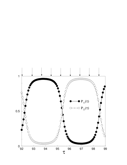
FIG. 6.: Integrated probability distributions of the spin $z$-components (diagonal components of the spin density matrix): $P_{11}(\tau)$, for $S_{z}=1/2$ ($\bullet$); and $P_{22}(\tau)$, for $S_{z}=-1/2$ ($\circ$), as functions of time. Vertical arrows show the time instants, $\tau_{k}=92.08+0.8k$, $k=0,1,...,8$ depicted in Fig. 5.

One might expect that the two peaks are associated with the functions $P_{n}(z,\tau)=|\Psi_{n}(z,\tau)|^{2}$, $n=1,2$. In fact the situation is more subtle: each function, $P_{n}(z,\tau)$ splits into two peaks. Fig. 5, shows these two functions for nine instants in time: $\tau_{k}=92.08+0.8k$, $k=0,1,...,8$. One can see the splitting of both $P_{1}(z,\tau)$ and $P_{2}(z,\tau)$; each peak of the function $P_{1}(z,\tau)$ has the same position as the two peaks of $P_{2}(z,\tau)$, but the amplitudes of these peaks differ. For instance for $k=1$ ($\tau=92.88$) the left-hand peak is dominantly composed of $P_{1}(z,\tau)$, while right hand peak is mainly composed of $P_{2}(z,\tau)$.

FIG. 7.: The dependence $\langle z(\tau)\rangle$ for the same values of parameters and initial conditions as in Figs 4-6.

With increasing time the relative contribution of each spin state to the two peaks varies. Fig. 6 shows the relative contribution of each spin state to the spatially integrated probability distributions: $P_{11}(\tau)=\int P_{1}(z,\tau)dz$ and $P_{22}(\tau)=\int P_{2}(z,\tau)dz$, as “truly continuous” functions of time, $\tau$. (Vertical arrows show the time instants, $\tau_{k}$.) It is important to note that the formation of the Schrödinger-cat state does not suppress, in the frameworks of the Scrödinger equation, the increase of the average amplitude, $\langle z(\tau)\rangle$, of the cantilever oscillations. Fig. 7, demonstrates the dependence $\langle z(\tau)\rangle$ for the same values of parameters and initial conditions as in Figs 4-6. We explored the affect of varying the initial state of the cantilever, including the effect of an initial state which is a superposition for the spin system, and found no significant affect on the Schrödinger-cat state dynamics. The value $|\alpha|$ cannot be significantly reduced if we are going to simulate a quasi-classical cantilever, and increasing $\alpha$ increases number of states $|n\rangle$ involved making simulation of the quantum dynamics more difficult. Our current basis includes 2000 states which allows accurate simulations.

V Summary

We consider the problem of a “truly continuous” measurement in quantum physics using the example of single-spin detection with a MRFM. Our investigation of the dynamics of a pure quantum spin 1/2 system interacting with a quasi-classical cantilever has revealed the generation of a quasi-periodic asymmetric Schrödinger-cat state for the measurement device.

In our example of the MRFM we considered the dynamics of a spin-cantilever system within the framework of the Schrödinger equation without any artificial assumptions. For a large number of spins, this equation describes the classical spin-cantilever dynamics, in good agreement with previous experimental results [17]. For single-spin detection, the Schrödinger equation describes the formation of a Schrödinger-cat state for the quasi-classical cantilever. In a realistic situation, the interaction with the environment may quickly destroy a Schrödinger-cat state of a macroscopic oscillator (see, for example, Refs. [20, 21]). In our case we would expect in a similar way that interaction with the environment would cause the wave function for the coupled spin-cantilever system to collapse, leading to a series of quantum jumps.

Finally, we discuss briefly the possible influence of the wave function collapse on the quantum dynamics of the spin-cantilever system. This collapse causes a sudden transformation of a two-peak probability distribution into a one peak probability distribution. It should be noted that the disappearance of the second peak does not produce a definite value of the $z$-component of the spin because both $P_{1}(z,t)$ and $P_{2}(z,t)$ contribute to both peaks (see Fig. 5). Thus, after the collapse of the wave function the spin does not jump into one of its two stationary states, $\left|\uparrow\right\rangle$ and $\left|\downarrow\right\rangle$, but is a linear combination of these states. Because of these quantum jumps, the cantilever motion (Fig. 7) which indicates detection of a single spin may be destroyed.

As the Schrödinger-cat state is highly asymmetric (the ratio of the peak areas is of the order 100) on average in 99 jumps out of 100 the probability distribution will collapse into the major peak. Such jumps change the integrated probabilities, $P_{11}$ and $P_{22}$, for the spin states with, $S_{z}=1/2$ and $S_{z}=-1/2$. However, this change does not affect the inequality between the values of $P_{11}$ and $P_{22}$: If $P_{11}$ is less that $P_{22}$ (or $P_{11}$ greater than $P_{22}$) before the collapse, the same inequality retains after the jump. On average, only in one out of 100 jumps (when the probability distribution collapses into the minor peak) the inequality between $P_{11}$ and $P_{22}$ reverses. After each collapse, the system evolves according to the Schrödinger equation until the Schrödinger-cat state appears causing the next collapse. To simulate the dynamics of the spin-cantilever system including quantum jumps, one should first estimate the characteristic decoherence time, $\tau_{d}$, i.e. the life-time of the Schrödinger-cat state taking into consideration the interaction with the environment. Then, one can choose a specific sequence of the life-times, $\tau_{dk}$, of the order $\tau_{d}$ and a specific sequence of the wave function collapses into the major and the minor peaks. (The probability of a collapse in any peak is proportional to the integrated area of a peak.) After this, one can consider quantum dynamics using Eqs (12) which generates the Schrödinger-cat state and interrupted by the collapse into one of the peaks. This rather phenomenological computational program repeated many times with different sequences of jumps could provide an adequate description of a possible experimental realization of a “truly continuous” quantum measurement which takes into account the interaction with the environment.

A movie demonstrating a Schrödinger-cat state dynamics can be found on the WEB:
www.dmf.bs.unicatt.it/ $\tilde{}$ borgonov/4cats.gif

REFERENCES

- [1] A. Peres, Continuous Monitoring of Quantum Systems, In: Information Complexity and Control in Quantum Physics, p. 235, Springer-Verlag, 1987.
- [2] V.B. Braginsky and F.Ya. Khalili, Quantum Measurement, Canbridge University Press, 1992.
- [3] M.B. Mensky, Continuous Quantum Measurements and Path Integrals, IOP Publishing, 1993.
- [4] D. Giulini, E. Joos, C. Kiefer, J. Kupsch, I.O. Stamatescu, and H.D. Zeh, Decoherence and the Appearance of a Classical World in Quantum Theory, Springer-Verlag, 1996.
- [5] C.C. Gerry and P.L. Knight, Am. J. of Phys., 65, 964 (1997).
- [6] K.K. Wan, R. Green, and C. Trueman, J. Opt. B: Quantum Semiclass. Opt., 2, 165 (2000).
- [7] C.J. Myatt, B.E. King, Q.A. Turchette, C.A. Sackett, D. Kielpinski, W.M. Itano, C. Monroe, and D.I. Wineland, NATURE , 403, 269, Jan. 20 (2000).
- [8] J.R. Friedman, V.Patel, W. Chen, S.K. Tolpygo, and J.E. Lukens, NATURE, 406, 43, July 6 (2000).
- [9] C.H. van der Wal, A.C.J. ter Haar, F.K. Wilhelm, R.N. Schouten, C.J.P.M. Harmans, T.P. Orlando, S. Loyd, J.E. Mooij, SCIENCE, 290, 773, Oct. 27 (2000).
- [10] A.J. Leggettt, Physics World, 23, Aug. (2000).
- [11] J. Audretsch, M. Mensky, and V. Namiot, Phys. Lett. A, 237 1 (1997).
- [12] M.B. Mensky, Physics-Uspekhi, 41 923 (1998) (Uspekhi Fizicheskkikh Nauk, 168, 1017 (1998).
- [13] S.A. Gurvitz, Phys. Rev. B, 56, 15215 (1997).
- [14] A.N. Korotkov, Quant-ph/9807051.
-
[15]
J.A. Sidles, Appl. Phys. Lett., 58, 2854 (1991);
Phys. Rev. Lett., 68, 1124 (1992). - [16] C. P. Slichter, Principles of Magnetic Resonance (Springer-Verlag, New York, 1989).
- [17] D. Rugar, O. Züger, S. Hoen, C.S. Yannoni, H.M. Vieth, and R.D. Kendrick, Science, 264, 1560 (1994).
- [18] G.P. Berman and V.I. Tsifrinovich, Phys. Rev. B, 61, 3524 (2000).
- [19] G.P. Berman, G.D. Doolen, P.C. Hammel, and V.I. Tsifrinovich, Phys. Rev. B, 61, 14694 (2000).
- [20] A.O. Caldeira and A.J. Leggett, Phys. Rev. A, 31, 1059 (1985).
- [21] W.H. Zurek, Physics Today, 44, 36 (1991).