Computer Model of Quantum Zeno Effect in Spontaneous Decay with Distant Detector

Abstract

A numerical model of spontaneous decay continuously monitored by a distant detector of emitted particles is constructed. It is shown that there is no quantum Zeno effect in such quantum measurement if the interaction between emitted particle and detector is short-range and the mass of emitted particle is not zero.

1 Introduction

The Quantum Zeno Paradox (QZP) is a proposition that evolution of a quantum system is stopped if the state of system is continuously measured by a macroscopic device to check whether the system is still in its initial state [1, 2]. QZP is a consequence of formal application of von Neumann’s projection postulate to represent a continuous measurement as a sequence of infinitely frequent instantaneous collapses of system’s wave function. It was shown theoretically [3] and experimentally [4] that sufficiently frequent discrete active measurements of system’s state really inhibit quantum evolution. This phenomenon was named ‘Quantum Zeno Effect’ (QZE). But the question about possibility of QZE during true continuous observations is not quite clear up to now.

A true continuous measurement of quantum system’s state takes place during observation of spontaneous decay by distant detector of emitted particles (another examples of continuous measurement of decay are presented in papers [5, 6, 7, 8, 9]). Let us consider a metastable exited atom surrounded for detectors to register an emitted photon (or electron) when the exited state of atom decays to the ground state. While the detectors are not discharged, the information that the atom is in its exited state is being obtained permanently, therefore the system’s state is being measured continuously. Could the presence of detectors influence on the decay constant of exited atom? If so, this would be the QZE in true continuous passive measurement.

It is impossible to describe this kind of continuous measurement by a sequence of discrete wave function collapses as was proposed in seminal works [1, 2]. Such approach leads to the explicit quantum Zeno paradox, not effect. Instead, a dynamical description of such measurements was elaborated in the number of works [10, 11, 12, 13]. In this approach object system (atom), radiation field (or emitted particle), and device (detector of particle) are considered as subsystems of one compound quantum system. The results of papers [10, 11] were mainly qualitative. The explicit expression for decay constant perturbed by given interaction $W$ of emitted particles with detector was obtained in [12, 13]. This expression is

$$\Gamma=2\pi\int d\omega M(\omega)\Delta(\omega-{\cal E}_{0}).$$ (1)

In Eq. (1) $M(\omega)$ is the sum of all transition matrix element squares related to the same energy of emitted particle $\omega$; ${\cal E}_{0}$ is the expectation value of final energy of emitted particle. The function $\Delta(\omega-{\cal E}_{0})$ describes the influence of observation on the decay constant. Without detector, i. e. $W=0$, the function $\Delta(\omega-{\cal E}_{0})$ transforms to Dirac’s delta-function $\delta(\omega-{\cal E}_{0})$ and Eq. (1) transforms to the Golden Rule [12, 13]. It was supposed [12] that the meaning of $\Delta(\omega-{\cal E}_{0})$ is an energy spreading of the final states of decay due to time-energy uncertainty relation and finite time-life of emitted particle until scattering on the detector. Then one can suggest that observation influences on decay in accordance with the following sequence: The faster detector, the shorter emitted particle time-life, the wider $\Delta(\omega-{\cal E}_{0})$, the stronger perturbation of decay constant.

It is clear that strong interactions $W$ is needed to obtain QZE. Hence, $W$ is essentially nonperturbative in this problem. This feature determines the main difficulty of calculations of function $\Delta(\omega-{\cal E}_{0})$ in Eq. (1) and, consequently, the perturbed value of decay constant. Particularly, in paper [12] we supposed that QZE explains strong inhibition of 76 eV-nuclear uranium-235 isomer decay in matrix of silver [14]. However, we had to restrict the consideration only by a qualitative analysis of Eq. (1) for this case because of difficulties of function $\Delta(\omega-{\cal E}_{0})$ calculations.

Since it is difficult to study realistic physical systems, it is reasonable to start with some simplified models to calculate the function $\Delta$. The aim of the present paper is strict and complete numerical investigation of Eq. (1) for a simple but not oversimplified model system. We derive Eq. (1), then introduce one-dimensional three-particle model of continuous observation of decay, then describe the numerical computation scheme for this model, and finally discuss results of calculations.

2 General considerations

In this section a derivation of Eq. (1) and other formulae to construct our numerical model are presented. Derivation of Eq. (1) is simplified in comparison with our previous papers [12, 13].

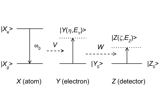
Figure 1: The compound system $S=X\otimes Y\otimes Z$ is the model of continuous observation of exited state $|X_{e}\rangle$ decay.

Let a compound system $S=X\otimes Y\otimes Z$ consists of three subsystems $X$, $Y$, and $Z$ (Fig. 1). The system $X$ (“atom”) decays spontaneously from the initial exited state $|X_{e}\rangle$ to the ground state $|X_{g}\rangle$ emitting a particle $Y$ (“electron”) due to interaction $V$ between systems $X$ and $Y$. This process is similar to autoionization decay of excited atomic state, but it is possible to suppose another nature of systems and interactions. The particle $Y$ is initially at the ground state $|Y_{0}\rangle$ (electron is on the bounded state in atom) and then transits to continuum $|Y(\eta,E_{Y})\rangle$. Here $E_{Y}$ is the energy of the state in the continuum and $\eta$ represents all other quantum numbers. Particle $Y$ inelastically scatters on third system $Z$ (“distant detector”) due to interaction $W$ between $Y$ and $Z$. As a result, the system $Z$ transits from the initial ground state $|Z_{0}\rangle$ to the continuum $|Z(\zeta,E_{Z})\rangle$. This transition is considered to be a registration of decay. We consider that the interaction $V$ does not effect on system $Z$, the interaction $W$ does not effect on system $X$ and the systems $Y$ and $Z$ don’t interact in their ground states. Therefore, we have

$$V=V_{XY}\otimes I_{Z};\quad W=I_{X}\otimes W_{YZ};\quad W_{YZ}|Y_{0}Z_{0}\rangle=0,$$ (2)

where $I_{X}$ and $I_{Z}$ are unit operators in the Hilbert spaces of corresponding systems. The Hamiltonian of whole system is

$$H=H_{0}+V+W,$$ (3)

where

$$H_{0}=H_{X}^{0}\otimes I_{YZ}+H_{Y}^{0}\otimes I_{XZ}+H_{Z}^{0}\otimes I_{YX}$$

with obvious notations.

The initial state of system $S$ at the initial moment of time $T=0$ is

$$|\Psi_{0}\rangle=|X_{e}\rangle\otimes|Y_{0}\rangle\otimes|Z_{0}\rangle\equiv|X_{e}Y_{0}Z_{0}\rangle.$$

Let us introduce the first order correction to the eigenenergy of state $|\Psi_{0}\rangle$ due to interaction $V$:

$$\delta V_{0}=\langle\Psi_{0}|V|\Psi_{0}\rangle$$

and renormalized unperturbed Hamiltonian $H_{0}$ and renormalized interaction $V$:

$$H_{0}^{\prime}=H_{0}+\delta V_{0}|\Psi_{0}\rangle\langle\Psi_{0}|;\quad V^{\prime}=V-\delta V_{0}|\Psi_{0}\rangle\langle\Psi_{0}|.$$

Then the Hamiltonian Eq. (3) may be rewritten as

$$H=H_{0}^{\prime}+V^{\prime}+W.$$

The initial state $|\Psi_{0}\rangle$ is an eigenstate of the Hamiltonian $H_{0}^{\prime}$ with the eigenenergy

$${\cal E}_{0}^{\prime}=E^{e}_{X}+E^{0}_{Y}+E^{0}_{Z}+\delta V_{0}.$$

The interaction $V$ is considered to be a small perturbation, but interaction $W$ is not small. To obtain the decay constant of the exited state $|X_{e}\rangle$ it is necessary to solve the Shrödinger equation for the whole system $S$. It is impossible to construct the perturbation theory for $W$, but it is possible for $V$. Therefore, let us introduce the interaction picture as ($\hbar=1$):

$$|\Psi_{I}(T)\rangle = {\rm e}^{i(H_{0}^{\prime}+W)T}|\Psi(T)\rangle,\quad|\Psi_{I}(0)\rangle=|\Psi_{0}\rangle$$ (4)

$$V_{I}^{\prime}(T) = {\rm e}^{i(H_{0}^{\prime}+W)T}V^{\prime}{\rm e}^{-i(H_{0}^{\prime}+W)T}.$$

Then the Shrödinger equation reads as

$$|\Psi_{I}(T)=|\Psi_{0}\rangle-i\int_{0}^{T}V_{I}^{\prime}(t)|\Psi_{I}(t)\rangle dt.$$ (5)

The solution of Eq. (5) in the second order of perturbation theory with respect to $V$ is

$$|\Psi_{I}(T)\rangle=|\Psi_{0}\rangle-i\int_{0}^{T}V_{I}^{\prime}(t)|\Psi_{0}\rangle dt-\int_{0}^{T}dt_{1}\int_{0}^{t_{1}}dt_{2}V_{I}^{\prime}(t_{1})V_{I}^{\prime}(t_{2})|\Psi_{0}\rangle.$$ (6)

Let $F(T)$ be no-decay amplitude

$$F(T)={\rm e}^{i{\cal E}_{0}^{\prime}T}\langle\Psi_{0}|\Psi(T)\rangle.$$

It follows from Eq. (4) and Eq. (6) that

$$F(T)=1-\int_{0}^{T}dt_{1}\int_{0}^{t_{1}}dt_{2}\langle\Psi_{0}|V_{I}^{\prime}(t_{1})V_{I}^{\prime}(t_{2})|\Psi_{0}\rangle.$$ (7)

For the initial region of exponential decay curve (time is not very small, not large) we assume

$$F(T)=\exp(-\gamma T)\cong 1-\gamma T,\;\gamma={\rm const}.$$ (8)

Then the quantity $\Gamma=2{\rm Re}\,\gamma$ is the probability of decay per unit of time (decay constant). Using Eq. (7) and Eq. (8), we obtain

$$\Gamma=2{\rm Re}\int_{0}^{\infty}\langle\Psi_{0}|V^{\prime}{\rm e}^{-i(H_{0}^{\prime}+W)t}V^{\prime}|\Psi_{0}\rangle{\rm e}^{i{\cal E}_{0}^{\prime}t}dt.$$ (9)

By $v(\eta,E_{Y})$ denote the matrix elements of $V$ which cause the decay of state $|X_{e}\rangle$ and emitting of particle $Y$:

$$v(\eta,E_{Y})=\langle X_{g}Y(\eta,E_{Y})|V^{\prime}_{XY}|X_{e}Y_{0}\rangle.$$ (10)

All other matrix elements don’t effect on the decay constant. Let us introduce the vector

$$|\widetilde{Y}\rangle=\int d\eta dE_{Y}|Y(\eta,E_{Y})\rangle v(\eta,E_{Y}).$$ (11)

Then, after simple algebraic transformations, Eq. (9) may be rewritten as

$$\Gamma=2\pi\int_{0}^{\infty}M(E_{Y})\Delta\left(E_{Y}-E_{Y}^{fin}\right)dE_{Y},$$ (12)

where

$$E_{Y}^{fin} = E_{Y}^{0}+\omega_{0}+\delta V_{0},\quad\omega_{0}=E^{e}_{X}-E^{g}_{X},$$

$$M(E_{Y}) = \int d\eta\left|v(\eta,E_{Y})\right|^{2},$$

$$\Delta(E) = \frac{1}{\pi}{\rm Re}\int_{0}^{\infty}D(t){\rm e}^{-iEt}dt,$$ (13)

$$D(t) = \frac{\langle\widetilde{Y}Z_{0}\left|{\rm e}^{-i(H_{YZ}^{0}+W_{YZ})t}\right|\widetilde{Y}Z_{0}\rangle}{\langle\widetilde{Y}Z_{0}\left|{\rm e}^{-iH_{YZ}^{0}t}\right|\widetilde{Y}Z_{0}\rangle},$$ (14)

$$H_{YZ}^{0} = H_{Y}^{0}\otimes I_{Z}+H_{Z}^{0}\otimes I_{Y}.$$

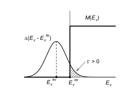
Figure 2: No-zero probability of decay forbidden by the Energy Conservation Law.

It is easily shown that $\int\Delta(E)dE=1$. We can not obtain an explicit analytical expression for $\Gamma$ with respect to the matrix elements of interaction $W$ due to nonperturbative character of this interaction. However, it is possible to derive an interesting qualitative conclusion on the shape of function $\Delta(E)$ (which is essentially used to calculate $\Gamma$) without calculations. For simplicity we suppose $M(E_{Y})$ to be a step-like function with the jump at energy $E_{Y}^{thr}$. Suppose the energy-spreading function $\Delta(E)$ be a bell-like and nearly symmetric with the maximum at $E=0$. Consider the case $E_{Y}^{fin}<E_{Y}^{thr}$ (Fig. 2). Then the transition $|X_{e}\rangle\to|X_{g}\rangle$ with emitting of particle $Y$ is strictly forbidden by the Energy Conservation Law. For example, the binding energy of atomic electron is greater than the transition energy $\omega_{0}$ and the electron can not be ionized during this transition. But the functions $\Delta(E_{Y}-E_{Y}^{fin})$ and $M(E_{Y})$ may have no-zero overlap integral Eq. (12) as is shown on Fig. 2. Hence $\Gamma>0$ and the transition $|X_{e}\rangle\to|X_{g}\rangle$ is possible. Thus, we come to a contradiction. This contradiction means that the suggestion about shape of function $\Delta(E)$ was wrong. The contradiction could be eliminated if whole no-zero part of function $\Delta(E)$ locates at the left-hand side of point $E=0$. Therefore, we conclude, that our formalisms predict this special shape for the function $\Delta(E)$. Another prediction is the following. Let $E_{Y}^{fin}-E_{Y}^{thr}>0$ but the value $E_{Y}^{fin}-E_{Y}^{thr}$ is of the order of function $\Delta(E)$ width or less. Then the transition $|X_{e}\rangle\to|X_{g}\rangle$ is permitted, but a considerable part of function $\Delta(E_{Y}-E_{Y}^{fin})$ is located at the left-hand side of point $E_{Y}^{thr}$, so $\Gamma<\Gamma_{0}$. Here $\Gamma_{0}$ is the decay constant not perturbed by the interaction of particle $Y$ with the device $Z$. This is QZE. In the following sections we will verify both predictions by direct calculations with a simple numerical model.

3 Numerical model

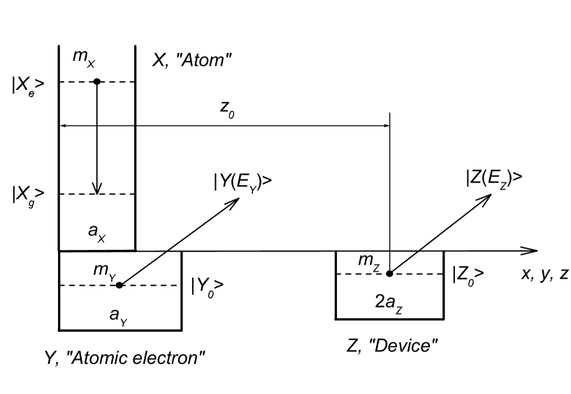
Figure 3: The one-dimensional three-particle model of spontaneous decay with continuous observation of decay particle by distant detector.

We consider one-dimensional three-particle model (Fig. 3) in this section and hereafter in present paper. The systems $X$, $Y$, $Z$ are one-dimensional rectangular potential wells. There is a single particle in each well in the initial state of system $X\otimes Y\otimes Z$. The masses of particles and the geometry of potential wells are clear from Fig. 3. We use the units such that $m_{Y}=1$, $a_{Y}=1$, $\hbar=1$. The coordinates of particles $X$, $Y$, $Z$ are denoted by $x$, $y$, $z$, respectively. There is infinitely high potential wall for all particles at the point $x=y=z=0$, consequently all particle eigenstates are no-degenerated. We consider that each particle $X$, $Y$, $Z$ governs only by its own potential well $U_{X}(x)$, $U_{Y}(y)$, $U_{Z}(z)$ respectively and by interparticle interactions.

The potential well $U_{X}(x)$ is a potential box with solid walls. The potential wells $U_{Y}(y)$ and $U_{Z}(z)$ are such that they contain only one bounded state for particles $Y$ and $Z$, respectively. The particles $X$ and $Y$ interact by repulsive $\delta$-like potential

$$V_{XY}(y-x)=v_{0}\delta(y-x),\quad v_{0}>0.$$ (15)

This interaction causes transition of particle $X$ from the initial state $|X_{e}\rangle$ to the ground state $|X_{g}\rangle$ and simultaneously excitation of particle $Y$ from the bounded state $|Y_{0}\rangle$ to the continuum $|Y_{e}(E_{Y})\rangle$. Since all states are no-degenerated, the degeneration index $\eta$ may be omitted. The threshold energy for particle $Y$ to be ionized is $E^{thr}_{Y}=0$. The particles $Y$ and $Z$ interacts by Gaussian repulsive potential

$$W_{YZ}(z-y) = P^{\prime}_{0}\,w_{0}\exp\left[-\frac{(z-y)^{2}}{2\sigma_{W}^{2}}\right]P^{\prime}_{0},\quad w_{0}>0;$$ (16)

$$P^{\prime}_{0} = (I_{YZ}-|Y_{0}Z_{0}\rangle\langle Y_{0}Z_{0}|).$$

The potential $W_{YZ}$ always fulfills the condition Eq. (2) due to the artificial factors $P^{\prime}_{0}$. We discuss these factors in the last section of paper. The Hamiltonian of joint system $X\otimes Y\otimes Z$ is

$$H = \left[-\frac{1}{2m_{x}}\frac{\partial^{2}}{\partial x^{2}}+U_{X}(x)\right]\otimes I_{YZ}+\left[-\frac{1}{2m_{y}}\frac{\partial^{2}}{\partial y^{2}}+U_{Y}(y)\right]\otimes I_{XZ}+$$

$$\left[-\frac{1}{2m_{z}}\frac{\partial^{2}}{\partial z^{2}}+U_{Z}(z)\right]\otimes I_{XY}+V_{XY}(y-x)\otimes I_{Z}+W_{YZ}(z-y)\otimes I_{X}.$$

General expressions for $v(\eta,E_{Y})$, $|\widetilde{Y}\rangle$, and $\Gamma$ (Eqs. (10,11,12) respectively) now become

$$v(E_{Y}) = \langle X_{g}Y(E_{Y})|V_{XY}|X_{e}Y_{0}\rangle,$$ (17)

$$|\widetilde{Y}\rangle = \int|Y(E_{Y})\rangle v(E_{Y})dE_{Y},$$ (18)

$$\Gamma = 2\pi\int|v(E_{Y})|^{2}\Delta(E_{Y}-E_{Y}^{fin})dE_{Y}.$$ (19)

The expressions for $\Delta(E)$ and $D(t)$ (Eqs. (13,14) respectively) are remain unchanged.

To calculate $\Gamma$ we should calculate $D(t)$. To calculate $D(t)$ we should calculate two functions

$$q(t) = \langle\widetilde{Y}Z_{0}|{\rm e}^{-i(H^{0}_{YZ}+W_{YZ})t}|\widetilde{Y}Z_{0}\rangle,$$ (20)

$$q_{0}(t) = \langle\widetilde{Y}Z_{0}|{\rm e}^{-iH^{0}_{YZ}t}|\widetilde{Y}Z_{0}\rangle$$ (21)

and then find $D(t)=q(t)/q_{0}(t)$. In this paper we calculate $q(t)$ numerically.

To calculate $q(t)$ the Shrödinger equation may be solved:

$$i\frac{\partial\widetilde{\Psi}(y,z,t)}{\partial t} = (H^{0}_{YZ}+W_{YZ})\widetilde{\Psi}(y,z,t)$$ (22)

$$\widetilde{\Psi}(y,z,0) = \widetilde{Y}(y)Z_{0}(z)$$ (23)

and then the inner product $q(t)=\langle\widetilde{Y}Z_{0}|\widetilde{\Psi}(y,z,t)\rangle$ may be obtained. It follows from Eqs. (15), (17), and (18) that $\widetilde{Y}(y)$ may be represented through functions $X_{e}$, $X_{g}$, and $Y_{0}$ as

$$\widetilde{Y}(y)=NY_{0}(y)\left[X^{*}_{g}(y)X_{e}(y)-\int|Y_{0}(y^{\prime})|^{2}X^{*}_{g}(y^{\prime})X_{e}(y^{\prime})dy^{\prime}\right],$$ (24)

where $N$ is a normalization factor. Since the functions $X_{e}(x)$, $X_{g}(x)$, $Y_{0}(y)$, and $Z_{0}(z)$ are well known eigenfunctions of one-dimensional rectangular well, it is easy to calculate the initial state Eq. (23) analytically. Note that it follows from Eq. (24) that $\widetilde{Y}(y)$ is a compact wave packet near the origin of axis $y$. The physical meaning of this wave packet is that it is the particle $Y$ state that arises virtually just after the particle excitation [12].

Eq. (22) was solved numerically. The state of the system $Y\otimes Z$ was represented by a grid wave function with zero margin conditions defined on two-dimensional equidistant rectangular grid with the same steps along $y$- and $z$-axis. Both dimensions $L_{Y}$ and $L_{Z}$ of calculation area were much greater than distance $z_{0}$ from the center of device $Z$ to the origin of coordinate system. The scheme of calculation was as follows. Let the grid wave function at the time $t$ be $\{\widetilde{\Psi}_{kl}(t)\}$ where $k=0,\dots,N_{Y}$; $l=0,\dots,N_{Z}$. Then the wave function at the time $t+\Delta t$ is calculated through successive four steps $(a),(b),(c),(d)$:
($a$) Calculation of sin-Fourier transform of the grid function $\{\widetilde{\Psi}_{kl}(t)\}$:

$$F_{mn}(t)=\frac{4}{N_{Y}N_{Z}}\sum_{k=1}^{N_{Y}-1}\sum_{l=1}^{N_{Z}-1}\widetilde{\Psi}_{kl}(t)\sin\left(\frac{m\pi}{N_{Y}}k\right)\sin\left(\frac{n\pi}{N_{Z}}l\right).$$

($b$) Calculation of free evolution of Fourier coefficients:

$$F_{mn}(t+\Delta t)=F_{mn}(t)\exp\left\{-i\left[\frac{1}{2m_{Y}}\left(\frac{m\pi}{L_{Y}}\right)^{2}+\frac{1}{2m_{Z}}\left(\frac{n\pi}{L_{Z}}\right)^{2}\right]\Delta t\right\}.$$

($c$) Calculation of back sin-Fourier transform that produces the free evolution of system $Y\otimes Z$ without potentials $U_{Y}$, $U_{Z}$, and $W_{YZ}$ during time interval $\Delta t$:

$$\widetilde{\Psi}^{\prime}_{kl}(t+\Delta t)=\sum_{k=1}^{N_{Y}-1}\sum_{l=1}^{N_{Z}-1}F_{mn}(t+\Delta t)\sin\left(\frac{m\pi}{N_{Y}}k\right)\sin\left(\frac{n\pi}{N_{Z}}l\right).$$

($d$) Calculation of contribution of all interactions to the evolution during time interval $\Delta t$:

$$\widetilde{\Psi}_{kl}(t+\Delta t)=\widetilde{\Psi}^{\prime}_{kl}\exp\{-i[U_{Y}(y_{k})+U_{Z}(z_{l})+W(z_{l}-y_{k})]\Delta t\}.$$

The zero margin conditions is fulfilled because of representation of $\{\widetilde{\Psi}_{kl}\}$ by sin-Fourier series.

The calculation of function $q_{0}(t)$ Eq. (21) is not difficult. This calculation may be carried out analytically or numerically by the same way as the calculation of function $q(t)$ but for $W_{YZ}=0$. To verify our calculation schemes both ways was tested (the results was identical).

To calculate the function $\Delta(E)$ through $D(t)$ one should calculate the Fourier transform Eq. (13). To do this we used the cubic spline approximation of the numerical function $D(t)$.

4 Results of calculations and discussion

Table 1: The parameters of problem for the models “Wide $W$” and “Narrow $W$”. Here $U^{0}_{Y}$ and $U^{0}_{Z}$ are the depths of wells $U_{Y}$ and $U_{Z}$.

Parameter	Wide $W$	Narrow $W$
$a_{X}$	$0.6$	$0.6$
$m_{Y}$	$1.0$	$1.0$
$a_{Y}$	$1.0$	$1.0$
$U^{0}_{Y}$	$-5.552$	$-5.552$
$E^{0}_{Y}$	$-2.776$	$-2.776$
$z_{0}$	$4.0$	$4.0$
$2a_{Z}$	$1.0$	$1.0$
$m_{Z}$	$0.9$	$0.9$
$U^{0}_{Z}$	$-2.210$	$-2.210$
$E^{0}_{Z}$	$-1.0$	$-1.0$
$\sigma_{W}$	$2.548$	0.2
$w_{0}$	$789.2$	20000

We present the results of calculations for two sets of parameters of problem (Table 1). All parameters were the same for both calculations except the parameters of interaction $W$. The first variant was the “Wide $W$”. For this variant $W$ was wide enough for particle $Z$ in its ground state $|Z_{0}\rangle$ to feel the appearance of the particle $Y$ in the continuum spectrum near the origin of coordinate system. Also, $W$ was strong enough to ionize the particle $Z$ from its ground state. The second variant was the “Narrow $W$”. For this case $W$ was narrow enough that the particle $Z$ does not feel the particle $Y$ near the origin of coordinate system. Also, $W$ was strong enough for particle $Y$ could not be tunnelled through particle $Z$ and the energy of transition $\omega_{0}$ was high enough to ionize $Z$.

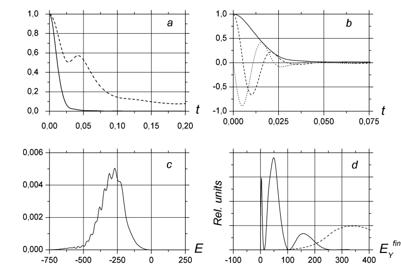
Figure 4: The calculations for “Wide $W$”. $(a)$: solid line—$|q(t)|$, dashed line—$|q_{0}(t)|$; $(b)$: solid line—$|D(t)|$, dashed line—${\rm Re}\,D(t)$, dotted line—${\rm Im}\,D(t)$; $(c)$: $\Delta(E)$; $(d)$: solid line—dependency of unperturbed value of decay constant $\Gamma_{0}$ on final energy $E^{fin}_{Y}$, dashed line—dependency of perturbed value $\Gamma$ on $E^{fin}_{Y}$. $\Gamma(E^{fin}_{Y})\approx 0$ for $0<E^{fin}_{Y}<100$ (Zeno effect).

The results of “Wide $W$” calculation is presented on Fig. 4. One can see from Fig. 4$a$ that the function $q(t)$ drops down faster then the function $q_{0}(t)$. This is a result of detector $Z$ excitation due to the interaction $W_{YZ}$ between the particle $Y$ and the detector $Z$ (see Eqs. (20,21)). As a result, the absolute value of function $D(t)=q_{0}(t)/q(t)$ drops down from the initial value $1.0$ to zero (Fig. 4$b$). At the same time the imaginary and real parts of $D(t)$ oscillate. The function $\Delta(E)$ (Fig. 4$c$) is a Fourier transform of $D(t)$ (Eq. (13)), therefore this function is bell-like due to dropping of function $D(t)$ and has left-side shift due to oscillations of real and imaginary part of $D(t)$. Moreover, it is seen from Fig. 4$c$ that $\Delta(E)\approx 0$ for $E>0$, as it was predicted on the base of Energy Conservation Law in Section 2.

One can change the transition energy $\omega_{0}$ of system $X$ by altering the particle mass $m_{X}$. Then the final energy $E^{fin}_{Y}\approx\omega_{0}-|E^{0}_{Y}|$ of particle $Y$ is changed simultaneously. Therefore, it is possible to consider the dependency of decay constants on $E^{fin}_{Y}$. The dependency of unperturbed decay constant $\Gamma_{0}$ (i. e. for $W_{YZ}=0$) on $E^{fin}_{Y}$ is shown on Fig. 4$d$ by solid line. The complicated shape of this function is a consequence of particle $Y$ reflection from the sharp margins of $U_{Y}$ potential well. The dependency of decay constant $\Gamma$ perturbed by interaction $W_{YZ}$ on $E^{fin}_{Y}$ is shown on Fig. 4$d$ by dashed line. It is seen that $\Gamma(E^{fin}_{Y})$ is strongly inhibited in comparison with $\Gamma_{0}$ for values of $E^{fin}_{Y}$ which are less then approximately 100. This is the predicted in Section 2 Zeno effect. Zeno effect in spontaneous decay takes place for low energies of decay particles, near the threshold of decay, if this effect is presented at all.

The model with “Wide $W$” interaction does not contradict any fundamental principles of quantum theory, but this model is quite unrealistic practically. The long distance interaction between $Y$ and $Z$ must couple the ground states $|Y_{0}\rangle$ and $|Z_{0}\rangle$ of systems $Y$ and $Z$ inevitably. To obtain $W_{YZ}|Y_{0}Z_{0}\rangle=0$ we inserted the artificial factors $(I_{YZ}-|Y_{0}Z_{0}\rangle\langle Y_{0}Z_{0}|)$ into the interaction $W_{YZ}$ in Eq. (16). It would be more realistic to consider sufficiently narrow interaction $W_{YZ}$ to obtain by natural way

$$w_{0}\exp\left[-\frac{(z-y)^{2}}{2\sigma_{W}^{2}}\right]Y_{0}(y)Z_{0}(z)\approx 0.$$

Figure 5: The calculations for “Narrow $W$”. Solid line—$D(t)$; dashed line—$P_{sur}(t)$.

Then the factors $(I_{YZ}-|Y_{0}Z_{0}\rangle\langle Y_{0}Z_{0}|)$ may be omitted, they do not play a role any more. To consider this realistic situation we studied the model of “Narrow $W$” with $\sigma_{W}=0.2$. It is seen that $\sigma_{W}\ll z_{0}$. The results of calculation with “Narrow $W$” was quite different from “Wide $W$” ones. The function $q(t)$ occurred to be almost the same as function $q_{0}(t)$. The resulting function $D(t)$ is shown on Fig. 5 by solid line. It is seen that $D(t)$ does not show a drop-down behavior, but rather shows some oscillations at long times. It is impossible to calculate the function $\Delta(E)$ numerically in this situation, because the integral Eq. (13) diverges, but it is clear that $\Delta(E)$ will be $\delta$-like, not spreaded bell-like function. Thus, $\Gamma$ and $\Gamma_{0}$ are almost equal each other and Zeno effect is absent in “Narrow $W$” model.

We mentioned that it would be reasonably to consider the function $\Delta(E_{Y}-E^{fin}_{Y})$ in Eq. (12) as an energy spreading of final state of decay due to a finite time life of particle $Y$ until inelastic scattering on detector $Z$. Then the sense of function $D(t)$ is the effective “decay curve” of the final state of decay in the analogy with the decay onto an unstable level [13]. But it is clearly seen that it is not the case for the model of “Narrow $W$”. Survival probability of the state $|Z_{0}\rangle$ after decay of the system $X$ was occur, may be written as

$$P_{sur}(t)={\rm Tr}\,[|Z_{0}\rangle\langle Z_{0}|\rho_{Z}(t)]=\int dy\left|\int dz\widetilde{\Psi}(y,z,t)Z_{0}^{*}(z)\right|^{2},$$

where $\widetilde{\Psi}(y,z,t)$ is the solution of Eq. (20) and $\rho_{Z}(t)$ is the reduced density matrix of the system $Z$. The curve $P_{sur}(t)$ is shown on Fig. 5 by dashed line. It is seen that the survival probability decreases with time (as could be expected) and that $P_{sur}(t)$ is quite different from the function $D(t)$.

A general cause of the found $D(t)$ behavior is the following. Note that for the model of “Wide $W$” the cause of $D(t)$ dropping down is excitation of system $Z$. We would expect that the same reason may lead to dropping of $D(t)$ in the model of “Narrow $W$” as well. Now consider the right hand side (RHS) term in Eq. (20). The function $\widetilde{Y}(y)$ is a compact wave packet near the origin of coordinate system. This packet contains both low-energy and high-energy components. Hence, the wave packet $\widetilde{Y}(y)$ does not drive with time from the left to the right along the $y$-axis, but spreaded out by the manner that the lowest energy part retains near the origin of coordinate system forever. This is a consequence of $m_{Y}>0$. Namely this lowest energy part of wave packet determines the value of inner product in the RHS of Eq. (20) and, consequently, behavior of $D(t)$. But this lowest energy part of wave packet can not influence on the state of system $Z$ due to a short range of interaction $W_{YZ}(z-y)$ and large length of distance $z_{0}$ (Fig. 3). As a result there is no influence of system $Z$ excitation to the behavior of function $D(t)$. Oscillations of $D(t)$ (Fig. 5) is appeared to be a result of elastic reflection of particle $Y$ from the particle $Z$ in its ground state $|Z_{0}\rangle$.

Thus, our conclusions are as follows. Firstly, the functions $\Delta(E)$ and $D(t)$ in Eqs. (12,13) have no any simple physical sense in the context of problem of continuous observation of decay by distant detector. Generally, the function $D(t)$ does not mean the survival of the final state of decay with time generally, and the function $\Delta(E)$ does not mean the energy spreading of decay final states. Secondly, there is no quantum Zeno effect during the continuous observation of spontaneous decay by distant detector if interaction between emitted particle and detector is short-range and the emitted particle has no-zero mass. Thirdly, Zeno effect in the context of the same problem takes place if the interaction between emitted particle and detector is long-range, but this situation is considered as unrealistic. Finally, we did not consider the case of “spreaded” detector, when the detector is represented by some medium which contains a decay system and we did not consider the case of massless emitted particles. The existence of Zeno effect in these situations is meanwhile an open question.

ACKNOWLEDGMENTS

The author acknowledges the fruitful discussions with M. B. Mensky and J. Audretsch and is grateful to V. A. Arefjev for the help in preparation of the paper. The work was supported in part by the Russian Foundation of Basic Research, grant 98-01-00161.

References

- [1] B. Misra and E. C. G. Sudarshan, J. Math. Phys. 18 (1977) 756.
- [2] C. B. Chiu, E. C. G. Sudarshan, and B. Misra, Phys. Rev. D 16 (1977) 520.
- [3] R. J. Cook, Phys. Scr. 21 (1988) 49.
- [4] W. M. Itano, D. J. Heinzen, J. J. Bollinger, and D. J. Wineland, Phys. Rev. A 41 (1990) 2295.
- [5] E. Mihokova, S. Pascazio, and L. S. Schulman, Phys. Rev. A 56 (1997) 25.
- [6] S. Pascazio and P. Facchi, Acta Physica Slovaca 49 (1999) 557.
- [7] M. B. Mensky, Physics Letters A 257 (1999) 227.
- [8] B. Elattari and S. A. Gurvitz, quant-ph/9908054 (1999).
- [9] B. Elattari and S. A. Gurvitz, quant-ph/0001020 (2000).
- [10] K. Kraus, Found. Phys. 11 (1981) 547.
- [11] A. Sudbery, Annals of Physics 157 (1984) 512.
- [12] A. D. Panov, Annals of Physics 249 (1996) 1.
- [13] A. D. Panov, Physics Letters A 260 (1999) 441.
- [14] V. V. Kol’tson and A. A. Rimsky-Korsakov, Izv. Akad. Nauk SSSR, Ser. Fiz. 53 (1989) 2085.