Measuring the Quantum State
of a Large Angular Momentum

Abstract

We demonstrate a general method to measure the quantum state of an angular momentum of arbitrary magnitude. The $(2F+1)\times(2F+1)$ density matrix is completely determined from a set of Stern-Gerlach measurements with $(4F+1)$ different orientations of the quantization axis. We implement the protocol for laser cooled Cesium atoms in the $6S_{1/2}(F=4)$ hyperfine ground state and apply it to a variety of test states prepared by optical pumping and Larmor precession. A comparison of input and measured states shows typical reconstruction fidelities ${\cal F}\gtrsim 0.95$.

The quantum state of a physical system encodes information which can be used to predict the outcome of measurements. The inverse problem was mentioned by Pauli already in 1933 [1]: is it possible to uniquely determine an unknown quantum state by measuring a sufficiently complete set of observables on a number of identically prepared copies of the system? This very basic question has gained new relevance in recent years, following the realization that systems whose components and evolution are manifestly quantum can perform tasks that are impossible with classical devices, such as certain computations, secure communication and teleportation [2]. As we harness quantum coherent dynamics for such purposes, the development of techniques to accurately control and measure quantum states becomes a matter of practical as well as fundamental interest. Reconstruction of a (generally mixed) quantum state based on a record of measurements is a nontrivial problem with no general solution [3], but system-specific algorithms have been developed and demonstrated experimentally in a limited number of cases. These include light fields [4], molecular vibrations [5], electron orbital motion [6], and center-of-mass motion in ion traps [7] and atomic beams [8]. More recently multi-particle quantum states have been measured for entangled spin-1/2 systems in NMR [9] and for polarization-entangled photon pairs [10].

In this letter we present a new experimental method to measure the unknown quantum state for an angular momentum of arbitrary magnitude. The protocol is implemented for laser cooled Cesium atoms in the $6S_{1/2}(F=4)$ hyperfine ground state, and typically reproduces input test states with a fidelity better than 0.95. Our work is motivated in part by our ongoing study of quantum transport and quantum coherence in magneto-optical lattices, where the atomic spin degrees of freedom couple to the center-of-mass motion [11]. The correlation between spin and motion in this system offers the possibility to use the angular momentum as a ‘meter’ in the sense introduced by von Neumann [12], to probe the spinor wavepacket dynamics. A similar application has been proposed in cavity QED, where an atomic angular momentum can be used to read out the quantum state of light in an optical cavity [13]. We expect our technique also to provide a powerful experimental tool to evaluate the performance and error modes of quantum logic gates for neutral atoms [14].

The angular momentum quantum state of an ensemble of atoms with spin quantum number $F$ is described by its density matrix $\varrho$. Newton and Young have shown that sufficient information to determine $\varrho$ can be extracted from a set of $4F+1$ Stern-Gerlach measurements, carried out with different orientations of the quantization axis [15]. They derived an explicit solution for quantization directions $\hat{n}_{k}$ with a fixed polar angle $\theta$ and evenly distributed azimuthal angles $\phi_{k}$. Our reconstruction algorithm uses the same general approach, but takes advantage of a simple numerical method to solve for the density matrix for a less restrictive choice of directions. This allows for flexibility in the experimental setup and improves the robustness against errors. As a starting point for our reconstruction we choose a space fixed coordinate system $\{\hat{x},\hat{y},\hat{z}\}$ in which to determine $\varrho$. If we perform a Stern-Gerlach measurement with the quantization axis along $\hat{z}$, we obtain the populations of the $2F+1$ eigenstates $|m_{z}\rangle$ of $\hat{F}_{z}$, i.e., the diagonal elements of the density matrix $\varrho$. Information about the off-diagonal elements can be extracted from additional Stern-Gerlach measurements with quantization axes along directions $\hat{n}_{k}\neq\hat{z}$. For each of these measurements we obtain a new set of populations $\pi_{m}^{(k)}$, corresponding to the diagonal elements of a matrix $\varrho^{(k)}$ representing $\varrho$ in a rotated coordinate system with the quantization axis oriented along $\hat{n}_{k}$. The associated coordinate transformation is a rotation by an angle $\theta_{k}$ around an axis $\hat{u}_{k}$ in the xy-plane and perpendicular to $\hat{n}_{k}$ [see Fig. 1(a)]. The new populations can then be found from a unitary transformation of $\varrho$,

$$\pi_{m}^{(k)}=\langle m|R^{(k)\dagger}\varrho R^{(k)}|m\rangle=\sum_{i,j}R^{(k)*}_{im}R_{jm}^{(k)}\varrho_{ij},$$ (1)

where $-F\leq m,i,j\leq F$ and $1\leq k\leq 4F+1$. The rotation operators are given by $R^{(k)}=\exp{\left[-\frac{i}{\hbar}\theta_{k}\hat{\bf F}\hat{u}_{k}\right]}.$ Arranging all the populations $\pi_{m}^{(k)}$ and the density matrix elements into vectors $\vec{\pi}$ and $\vec{\rho}$, Eq. 1 can compactly be written as $\vec{\pi}={\mathbf{M}}\vec{\rho}$, where the elements of the rectangular matrix ${\mathbf{M}}$ are determined by the set of rotations $\{R^{(k)}\}$. The elements of the density matrix $\varrho$ can then be obtained as $\vec{\rho}={\mathbf{M}}^{+}\vec{\pi}$, where

$${\mathbf{M}}^{+}=\sum_{i=1}^{R}\frac{1}{\sqrt{\lambda_{i}}}\>{\mathbf{w}}_{i}\,{\mathbf{v}}_{i}^{\dagger}$$ (2)

is the Moore-Penrose pseudoinverse [16]. $R$ and $\lambda_{i}$ are the rank and non-zero eigenvalues of the Hermitian matrix ${\mathbf{M}}^{\dagger}{\mathbf{M}}$, with ${\mathbf{w}}_{i}$ and ${\mathbf{v}}_{i}$ being the corresponding eigenvectors of ${\mathbf{M}}^{\dagger}{\mathbf{M}}$ and ${\mathbf{M}}{\mathbf{M}}^{\dagger}$, respectively.

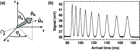
FIG. 1.: (a) Direction $\hat{n}_{k}$ of a Stern-Gerlach measurement in spherical coordinates. (b) Time-of-flight distribution with well separated peaks corresponding to the populations in the magnetic sublevels $|m\rangle$.

In a real experiment there is both random measurement noise and systematic errors, which cause the observed populations $\pi_{m}^{(k)}$ to deviate from those predicted by Eq. 1. In this situation the pseudoinverse solution yields a least-squares fit to the data [16]. This fit, however, will become sensitive to noise and errors if one or more of the $\lambda_{i}$ in Eq. 2 are too close to zero. A robust reconstruction algorithm must therefore use a set of directions $\{\hat{n}_{k}\}$ that lead to reasonably large $\lambda_{i}$. A second problem arises because the pseudoinverse solution, while always the best fit to the data, is not guaranteed to be a physically valid density matrix when noise and errors are present — a density matrix has unit trace, is Hermitian and has non-negative eigenvalues. The pseudoinverse solution automatically fulfills the first two conditions when the input populations are normalized. However, when negative eigenvalues occur we have to employ a different method to solve the inversion problem. For this purpose, we decompose $\varrho$ as

$$\varrho=TT^{\dagger} T_{ij}=0,\text{for }j>i,$$ with

and $$T_{ii}\in{\mathbb{R}},\,\,\sum_{i,j}|T_{ij}|^{2}=1.$$

This form automatically enforces the density matrix to have unit trace, be Hermitian and positive semi-definite. The $(2F+1)^{2}-1$ independent real-valued parameters of the complex, lower-triangular matrix $T$ can then be optimized to yield the best fit between measured and expected populations.

We have implemented this general procedure for Cesium atoms in the $6S_{1/2}(F=4)$ hyperfine ground state manifold. A standard magneto-optical trap (MOT) and optical molasses setup is used to prepare an ensemble of $\sim$10⁶ atoms in a volume of $0.1\text{\, mm}^{3}$ and at a temperature of $3.5\mu\text{K}$. Atoms from the molasses are loaded into a near-resonance optical lattice, composed of a pair of laser beams with orthogonal linear polarizations (1D lin$\perp$lin configuration) and counter-propagating along the (vertical) z-axis. Following this second laser cooling step the atoms are released from the lattice, at which point a range of angular momentum quantum states can be produced as discussed below. To allow accurate preparation and manipulation of these test states, we measure and compensate the background magnetic field in our setup to better than 1 mG.

A laser cooling setup provides a convenient framework for Stern-Gerlach measurements [17]. At the beginning of each measurement we define the quantization axis by applying (switching time $\sim$2 $\mu$s) a homogeneous bias magnetic field of $\sim$1 G pointing in the desired direction. All subsequent changes in the magnetic field are adiabatic, which ensures that the initial projection of the atomic spin onto the direction of the field is preserved at later times. As the atoms fall under the influence of gravity, we apply a strong magnetic field gradient ($|{\mathbf{B}}|\approx 100\text{ G and }\nabla|{\mathbf{B}}|\approx 100$ G/cm ) by pulsing on the MOT coils for 15 ms. The resulting state dependent force ${\mathbf{F}}=-mg_{F}\mu_{\text{B}}\nabla|{\mathbf{B}}|$ is sufficient to completely separate the arrival times for atoms in different $|m\rangle$ as they fall through a probe beam located 6.9 cm below the MOT volume [see Fig. 1(b)]. The magnetic populations can then be accurately determined from a fit to each separate arrival distribution. In our case a total of $4F+1=17$ Stern-Gerlach measurements are needed to reconstruct $\varrho$. The corresponding 17 different directions $\hat{n}_{k}$ of the bias magnetic field are produced by three orthogonal pairs of coils in near-Helmholtz configuration. This setup provides complete freedom to choose the measurement directions, and allows us to set the dc-magnetic field with an accuracy of $0.1^{\circ}$ in a volume of 1 cm${}^{3}.$ For the results reported below we use 16 measurements on a cone with $\theta_{k}\approx 82^{\circ}$, and a single measurement with $\theta_{k}=0^{\circ}$.

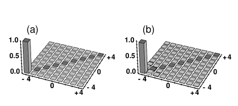
FIG. 2.: (a) Density matrix of a pure $|m_{z}=-4\rangle$ input state obtained by optical pumping with $\sigma^{-}$-polarized light, and (b) measured density matrix with a fidelity of ${\cal F}=0.97$. Note: All figures display absolute values of the density matrices.

We evaluate the performance of our reconstruction procedure by applying it to a number of known input states. These test states are created by a combination of laser cooling, optical pumping and Larmor precession in an externally applied magnetic field. First consider optical pumping by a $\sigma^{-}$-polarized laser beam tuned to the $6S_{1/2}(F=4)\to 6P_{3/2}(F^{\prime}=4)$ transition, which allows us to prepare the ensemble in a pure $|m_{z}=-4\rangle$ state. A single Stern-Gerlach measurement with quantization axis along $\hat{z}$ confirms the essentially unit population of this state. For a single non-zero population we can rule out off-diagonal elements due to the constraint $|\varrho_{ij}|^{2}\leq\varrho_{ii}\varrho_{jj}$, and in this case we therefore know the complete density matrix with a high degree of confidence. Both the input and measured density matrices are shown in Fig. 2, and show excellent agreement. To quantify the performance we use the fidelity [18]

$${\cal F}=\left(\text{Tr}\left[\sqrt{\varrho_{i}^{1/2}\varrho_{r}\varrho_{i}^{1/2}}\,\right]\right)^{2},$$

which is a measure of the closeness between the input ($\varrho_{i}$) and the reconstructed ($\varrho_{r}$) density matrices and takes on the value ${\cal F}=1$ when they are identical. For an $|m_{z}=-4\rangle$ input state our reconstruction fidelity is ${\cal F}=0.97$. Optical pumping with $\sigma^{+}$ yields a nearly pure $|m_{z}=4\rangle$ state, which we can similarly reconstruct with a fidelity of ${\cal F}=0.94$. Starting from $|m_{z}=-4\rangle$ we can further produce a range of spin-coherent states [19] by applying a magnetic field along, e.g., the x-axis and letting the state precess for a fraction of a Larmor period. Figure 3 shows the measured density matrices for four different precession angles, again with excellent reconstruction fidelity.

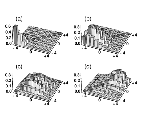
FIG. 3.: Measured density matrices for spin-coherent states obtained by a controlled Larmor precession of $|m=-4\rangle$ around $\hat{x}$ by (a) 30^∘ [${\cal F}=0.95$], (b) 60^∘ [${\cal F}=0.96$], (c) 90^∘ [${\cal F}=0.95$], and (d) 120^∘ [${\cal F}=0.92$].

It is desirable to also check the reconstruction of test states that are not quasi-classical, and whose density matrix exhibits large coherences far from the diagonal. One example of such a state is $|m_{y}=0\rangle$, which we can produce by optical pumping on the $F=4\to F^{\prime}=4$ transition with linear polarization along $\hat{y}.$ In this basis, the input test state has the density matrix shown in Fig. 4(a). Its representation in the $\{|m_{z}\rangle\}$ basis is easily found by a (numerical) rotation by $90^{\circ}$ around $\hat{x}$ [Fig. 4(c)], and can be directly compared to the reconstruction [Fig. 4(d)]. To simplify the visual comparison we finally rotate the measured density matrix by $-90^{\circ}$ around $\hat{x}$ to find its representation in the $\{|m_{y}\rangle\}$ basis [Fig. 4(b)]. The basis independent reconstruction fidelity is ${\cal F}=0.96$. The non-classical nature of the measured state is apparent in its Wigner function representation [20], which takes on negative values as shown in Fig. 5.

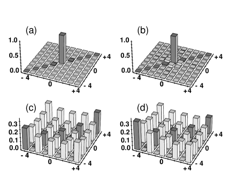
FIG. 4.: (a) Input state $|m_{y}=0\rangle$ prepared by optical pumping with linear $\hat{y}$-polarized light, and the reconstruction result (b) represented as density matrices in the $\{|m_{y}\rangle\}$ basis. The density matrices of input (c) and measured state (d) in the standard $\{|m_{z}\rangle\}$ basis. The fidelity is 0.96.

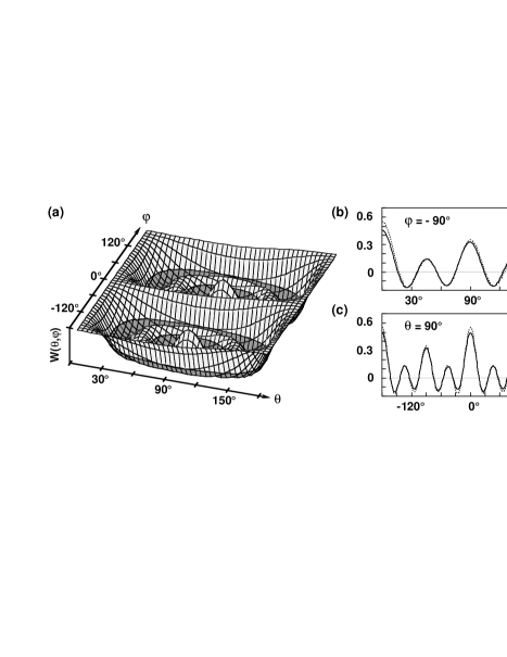
FIG. 5.: (a) Measured $|m_{y}=0\rangle$ state, represented by the Wigner function $W(\theta,\varphi)$ in spherical phase-space. The darker shading indicates negative values. Selected cuts of $W(\theta,\varphi)$ along (b) $\varphi=-90^{\circ}$ and (c) $\theta=90^{\circ}$ (dotted lines = input state, solid lines = measured state).

As a final test we have applied our procedure to the (presumably) mixed states that result from laser cooling. Figures 6(a,b) show the input and reconstructed states produced by laser cooling in a 1D lin$\perp$lin lattice. The input state shown here is based on a single Stern-Gerlach measurement of the magnetic populations, but it seems reasonable to assume that the highly dissipative laser cooling process destroys coherences between magnetic sublevels and that the density matrix is diagonal. Our measurement confirms this assumption. We can perform the same experiment with atoms released directly from a 3D optical molasses, in which case there is no preferred spatial direction and one expects something close to a maximally mixed state. Figures 6(c,d) show input and measured density matrices in good agreement with this assumption.

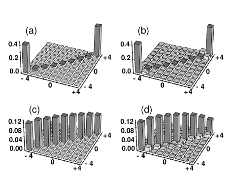
FIG. 6.: Mixed states: (a) input state from a near-resonance lattice, and (b) measured result. The apparent coherences are real and due to a 6.5^∘ tilt of the lattice with respect to $\hat{z}$. (c) Nearly maximally mixed state obtained from optical molasses phase, and (d) corresponding measured density matrix. Matrix comparisons of these mixed states each yield a fidelity of 0.99, however, the input state is known with less confidence.

In summary we have demonstrated a method to experimentally determine the complete density matrix of a large angular momentum, and tested its performance with a variety of angular momentum quantum states of an ensemble of laser cooled Cesium atoms in the $6S_{1/2}(F=4)$ hyperfine ground state. The input and reconstructed density matrices typically agree with a fidelity of ${\cal F}\gtrsim 0.95$. Limitations on the accuracy to which the density matrix can be measured appear to derive from $\approx 3\%$ uncertainties in the individual population measurements, and from variations in the direction of the bias magnetic field during the first few $\mu$s when it is turned on. These variations are likely due to induced currents in metallic fixtures and additional coils in the vicinity of our glass vacuum cell, and translate into uncertainty about the exact orientation of the quantization axes for the Stern-Gerlach measurements. Efforts are underway to eliminate these problems and achieve even better reconstruction fidelities.

We would like to thank K. Cheong, D. L. Haycock, H. H. Barrett, and the group of I. H. Deutsch at the University of New Mexico for helpful discussions. This research was supported by the NSF (9732612/9871360), ARO (DAAD19-00-1-0375) and JSOP (DAAD19-00-1-0359).

REFERENCES

- [1] W. Pauli, Handbuch der Physik (Springer, Berlin, 1933), Vol. 24(1), p. 98
- [2] Introduction to Quantum Computation and Information, edited by H.-K. Lo, S. Popescu, and T. Spiller (World Scientific, Singapore, 1998)
- [3] S. Weigert, Phys. Rev. A 45, 7688 (1992)
- [4] D. T. Smithey et al., Phys. Rev. Lett. 70, 1244 (1993); G. Breitenbach et al., J. Opt. Soc. Am. B 12, 2304 (1995)
- [5] T. J. Dunn, I. A. Walmsley, and S. Mukamel, Phys. Rev. Lett. 74, 884 (1995)
- [6] J. R. Ashburn et al., Phys. Rev. A 41, 2407 (1990)
- [7] D. Leibfried et al., Phys. Rev. Lett. 77, 4281 (1996)
- [8] C. Kurtsiefer, T. Pfau, and J. Mlynek, Nature 386, 150 (1997); R. A. Rubenstein et al., Phys. Rev. Lett. 83, 2285 (1999)
- [9] I. L. Chuang, N. Gershenfeld, and M. Kubinec, Phys. Rev. Lett. 80, 3408 (1998)
- [10] A. G. White et al., Phys. Rev. Lett. 83, 3103 (1999)
- [11] D. L. Haycock et al., Phys. Rev. Lett. 85, 3365 (2000); I. H. Deutsch et al., J. Opt. B 2, 633 (2000)
- [12] J. von Neumann, Mathematical Foundations of Quantum Mechanics (Princeton University Press, Princeton, 1955)
- [13] R. Walser, J. I. Cirac, and P. Zoller, Phys. Rev. Lett. 77, 2658 (1996)
- [14] G. K. Brennen et al., Phys. Rev. Lett. 82, 1060 (1999); D. Jaksch et al., ibid. 82, 1975 (1999)
- [15] R. G. Newton and B.-L. Young, Ann. Phys. (NY) 49, 393 (1968)
- [16] W. H. Press et al., in Numerical Recipes (Cambridge, 1992), Chap. 2.6
- [17] L. S. Goldner et al., Phys. Rev. Lett. 72, 997 (1994); D. L. Haycock et al., Phys. Rev. A 57, R705 (1998)
- [18] A. Uhlmann, Rep. Math. Phys. 9, 273 (1976); R. Josza, J. Mod. Opt. 41, 2315 (1994)
- [19] F. T. Arecchi et al., Phys. Rev. A 6, 2211 (1972)
- [20] J. P. Dowling, G. S. Agarwal, and W. P. Schleich, Phys. Rev. A 49, 4101 (1994) and references therein